
Calibration of Acoustic Emission Parameters in Relation to the Equilibrium Moisture Content Variations in a Pinus sylvestris Beam


Abstract
:1. Introduction
2. Materials and Methods
2.1. Experimental Setup
- Amplitude (A): is the peak in decibel during an acoustic emission event; it shows the disturbance level and the response of the sensor after power/energy loss. The set threshold value was 40 dB.
- Counts (C): it shows the number of times a signal exceeds a set threshold value. Real events have high counts.
- Energy (E): is the elastic energy released during an acoustic emission event, measured in arbitrary units (or energy units, e.u. = 10−14V2s). The AE energy can be determined using Equation (1), integrating the absolute or the squared values of the signal’s voltage curve over time [21]. Real events have high energy units.
2.2. Scots Pine Beam and Its Thermodinamic Equilibrium
2.2.1. Simil-CT Samplings of Scots Pine
2.2.2. Thermo-Dynamic Equilibrium of Moisture Content
2.3. Equilibrium Moisture Content Model and the Acoustic Emission Signals
3. Results and Discussions
3.1. Acoustic Emission Analysis
3.2. Gradient of the Equilibrium Moisture Content
3.3. Acoustic Emission vs. Equilibrium Moisture Content
4. Conclusions
- identify pre-existing macro or micro cracks in samples, which act as an open joint, reducing accumulated stress without emitting new acoustic emission events.
- point out damage caused by moisture variations, i.e., when the increasing ductility of the material generates no elastic energy.
Author Contributions
Funding
Acknowledgments
Conflicts of Interest
Appendix A


| Equation | ESTD | |
|---|---|---|
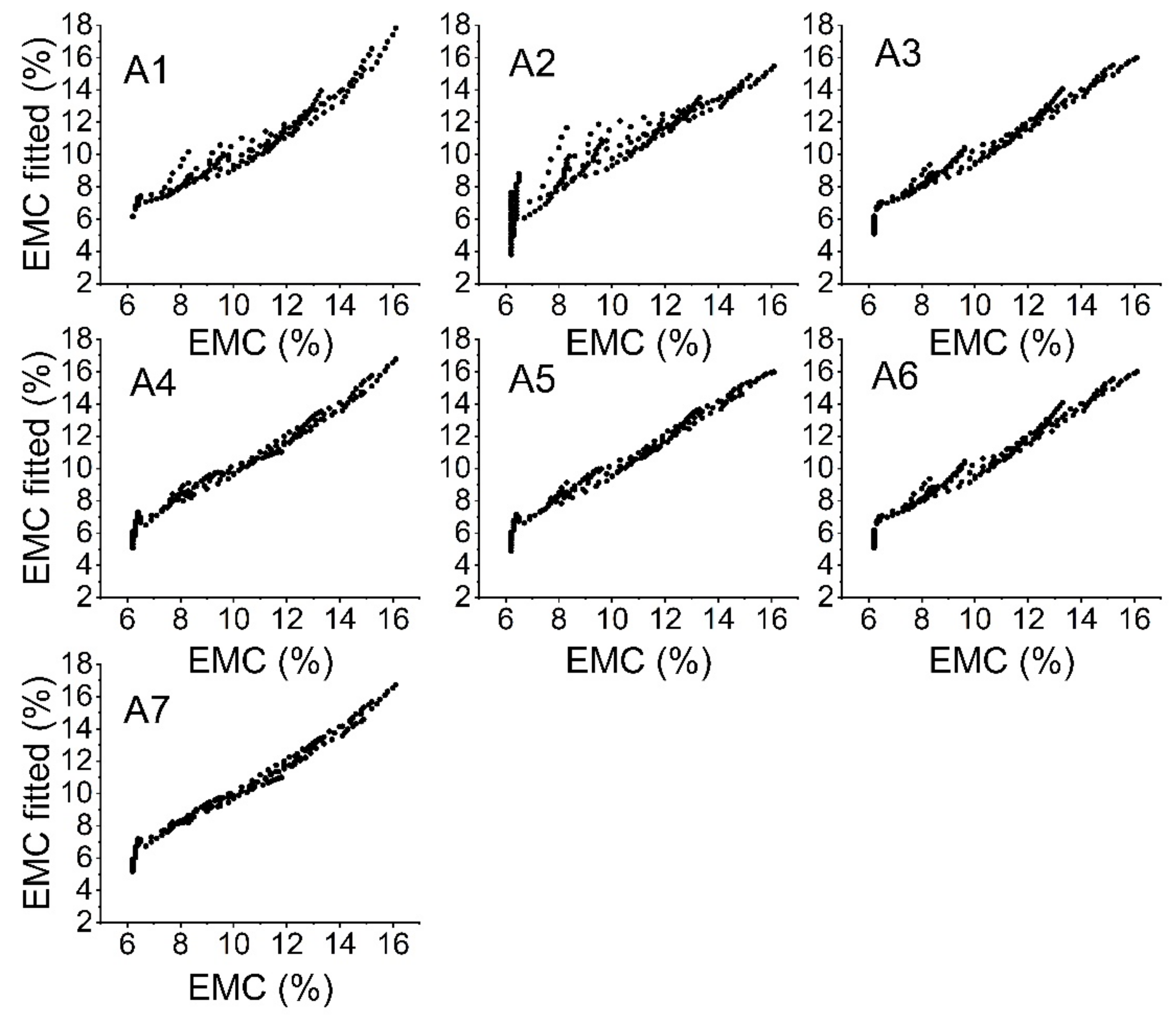
| (A1) | 0.96 | 0.59 |
| (A2) | 0.89 | 0.93 |
| (A3) | 0.98 | 0.42 |
| (A4) | 0.98 | 0.42 |
| (A5) | 0.98 | 0.37 |
| (A6) | 0.98 | 0.42 |
| (A7) | 0.98 | 0.38 |
| Equation | Coefficients (b) | |||||||
|---|---|---|---|---|---|---|---|---|
| Int. | x1 | x2 | x1∙x2 | x12 | x22 | x12 ∙x22 | ||
| (A1) | 6.06 | 1.33 × 10⁻² | −2.48 × 10⁻³ | 2.38 × 10⁻⁴ | ||||
| (A2) | 1.19 | 1.27 × 10⁻¹ | 1.06 × 10⁻² | −3.65 × 10⁻⁴ | ||||
| (A3) | 6.79 | −2.35 × 10⁻² | −7.89 × 10⁻³ | 5.09 × 10⁻⁴ | −3.97 × 10⁻⁹ | |||
| (A4) | 2.64 | 5.34 × 10⁻² | 1.68 × 10⁻² | 2.38 × 10⁻⁴ | −3.65 × 10⁻⁴ | −3.11 × 10⁻⁵ | ||
| (A5) | 4.94 | −1.16 × 10⁻² | 5.28 × 10⁻³ | 4.48 × 10⁻⁴ | −3.27 × 10⁻⁵ | −1.93 × 10⁻⁵ | −3.07 × 10⁻⁹ | |
| (A6) | 6.79 | −2.35 × 10⁻² | −7.89 × 10⁻³ | 5.09 × 10⁻⁴ | −3.97 × 10⁻⁹ | |||
| (A7) | 3.15 | 9.41 × 10⁻² | 1.98 × 10⁻¹ | 1.14 × 10⁻⁴ | −4.60 × 10⁻⁵ | −1.61 × 10⁻⁵ | −1.88 × 10⁻¹ | |
References
- Cagnana, A.I.L. Archeologia dei Materiali da Costruzione; S.A.P. Società Archeologica s.r.l.: Mantova, Italy, 2000; pp. 215–231. [Google Scholar]
- Berti, S. Le Biomasse Legnose: Il Legno; Volume Biomasse Forestali ad Uso Energetico in Ambiente Alpino: Potenzialità e Limiti; Consiglio Nazionale delle Ricerche (CNR): Rome, Italy, 4 June 2007. [Google Scholar]
- SyMBoL–Sustainable Management of Heritage Buildings in a Long-Term Perspective-NTNU. Available online: https://www.ntnu.edu/symbol (accessed on 9 April 2021).
- Dario, C.; Limpens-Neilen, D.; Shellen, H.L. Roman, Kozlowsky Church Heating and the Preservation of the Cultural Heritage Guide to the Analysis of the Pros and Cons of Various Heating Systems; Electa: Milan, Italy, 2007; ISBN 88-370-5034-8. [Google Scholar]
- Bartolucci, B.; De rosa, A.; Bertolin, C.; Berto, F.; Penta, F.; Siani, A.M. Mechanical Properties of the Most Common European Woods: A Literature Review. Frat. Ed Integrità Strutt. 2020, 54, 249–274. [Google Scholar] [CrossRef]
- Li, Z.; Jiang, J.; Lyu, J.; Cao, J. Orthotropic Viscoelastic Properties of Chinese Fir Wood Saturated with Water in Frozen and Non-Frozen States. For. Prod. J. 2021, 71, 77–83. [Google Scholar] [CrossRef]
- Li, X.; Li, M.; Ju, S. Frequency Domain Identification of Acoustic Emission Events of Wood Fracture and Variable Moisture Content. For. Prod. J. 2020, 70, 107–114. [Google Scholar] [CrossRef]
- Jakieła, S.; Bratasz, Ł.; Kozłowski, R. Acoustic Emission for Tracing Fracture Intensity in Lime Wood Due to Climatic Variations. Wood Sci. Technol. 2008, 42, 269–279. [Google Scholar] [CrossRef]
- Jakiela, S.; Bratasz, L.; Kozlowski, R. Acoustic Emission for Tracing the Evolution of Damage in Wooden Objects. Stud. Conserv. 2007, 52, 101–109. [Google Scholar] [CrossRef]
- Łukomski, M.; Strojecki, M.; Pretzel, B.; Blades, N.; Beltran, V.; Freeman, A. Acoustic Emission Monitoring of Micro-Damage in Wooden Art Objects to Assess Climate Management Strategies. Insight Non Destr. Test. Cond. Monit. 2017, 59, 256–264. [Google Scholar] [CrossRef]
- Perrin, M.; Yahyaoui, I.; Gong, X. Acoustic Monitoring of Timber Structures: Influence of Wood Species under Bending Loading. Constr. Build. Mater. 2019, 208, 125–134. [Google Scholar] [CrossRef]
- Barbosh, M.; Sadhu, A.; Sankar, G. Time–Frequency Decomposition-Assisted Improved Localization of Proximity of Damage Using Acoustic Sensors. Smart Mater. Struct. 2021, 30, 025021. [Google Scholar] [CrossRef]
- El-Hadad, A.; Brodie, G.I.; Ahmed, B.S. The Effect of Wood Condition on Sound Wave Propagation. Open J. Acoust. 2018, 8, 37. [Google Scholar] [CrossRef] [Green Version]
- Yang, L.; FeiYun, X. Acoustic emission signal characteristics of Pinus yunnanensis with different moisture content. Sci. Silvae Sin. 2019, 55, 96–102. [Google Scholar]
- Li, X.; Ju, S.; Luo, T.; Li, M. Effect of Moisture Content on Propagation Characteristics of Acoustic Emission Signal of Pinus Massoniana Lamb. Eur. J. Wood Wood Prod. 2020, 78, 185–191. [Google Scholar] [CrossRef]
- Bertolin, C.; De Ferri, L.; Berto, F. Calibration Method for Monitoring Hygro-Mechanical Reactions of Pine and Oak Wood by Acoustic Emission Nondestructive Testing. Materials 2020, 13, 3755. [Google Scholar] [CrossRef] [PubMed]
- Aicher, S.; Höfflin, L.; Dill-Langer, G. Damage Evolution and Acoustic Emission of Wood at Tension Perpendicular to Fiber. Holz Als Roh Werkst. 2001, 59, 104–116. [Google Scholar] [CrossRef]
- MTS Criterion® Series 40 Electromechanical Universal Test Systems. Available online: https://test.mts.com/-/media/materials/pdfs/brochures/100-262-929d_criterionem40.pdf?as=1 (accessed on 9 April 2021).
- Stingray. The Transformer Camera. Available online: https://www.1stvision.com/cameras/AVT/dataman/Stingray_DataSheet_F504BC_fiber_V1.1.1.pdf (accessed on 9 April 2021).
- AMSY-6 System Description. Available online: https://www.vallen.de/zdownload/pdf/AMSY-6_Description.pdf (accessed on 9 April 2021).
- Baensch, F. Damage Evolution in Wood and Layered Wood Composites Monitored in Situ by Acoustic Emission, Digital Image Correlation and Synchrotron Based Tomographic Microscopy. Ph.D. Thesis, ETH Zurich, Zurich, Switzerland, 2015. [Google Scholar]
- Kretschmann, D.E. Mechanical Properties of Wood. In Wood Handbook, Wood as an Engineering Material; Forest Products Laboratory: Madison, WI, USA, 2010; pp. 1–44. [Google Scholar]
- Tresenteret. Available online: http://www.tresenter.no/aktuelt/ntnu-og-tresenteret-etablerer-nytt-senter-ntnu-wood (accessed on 9 April 2021).
- Camuffo, D. Thermodynamics for Cultural Heritage. In Physics Methods in Archaeometry; Martini, M., Milazzo, M., Piacentini, M., Eds.; IOS Press: Varenna, Italy; Amsterdam, The Netherlands, 2004; pp. 37–98. [Google Scholar]
- Marco, M. Climate Risk Assessment in Museums: Degradation Risks Determined from Temperature and Relative Humidity Data; Technische Universiteit Eindhoven: Eindhoven, The Netherlands, 2012. [Google Scholar]
- Giordano, G. Tecnologia Del Legno. La Materia Prima; UTET: Torino, Italy, 1981; Volume 1. [Google Scholar]
- Camuffo, D. Microclimate for Cultural Heritage-Measurments, Risk Assessment, Conservation, Restoration, and Maintenance of Indoor and Outdoor Monuments, 3rd ed.; Elsevier: Amsterdam, The Netherlands, 2019. [Google Scholar]
- Li, S.; Wu, G.; Shi, H. Acoustic Emission Characteristics of Semi-Rigid Bases with Three Moisture Conditions during Bending Tests. Road Mater. Pavement Des. 2017, 20, 187–198. [Google Scholar] [CrossRef]


| ID Number | Group | Directionality | Grain Angle | |
|---|---|---|---|---|
| 50th percentile | 90th percentile | |||
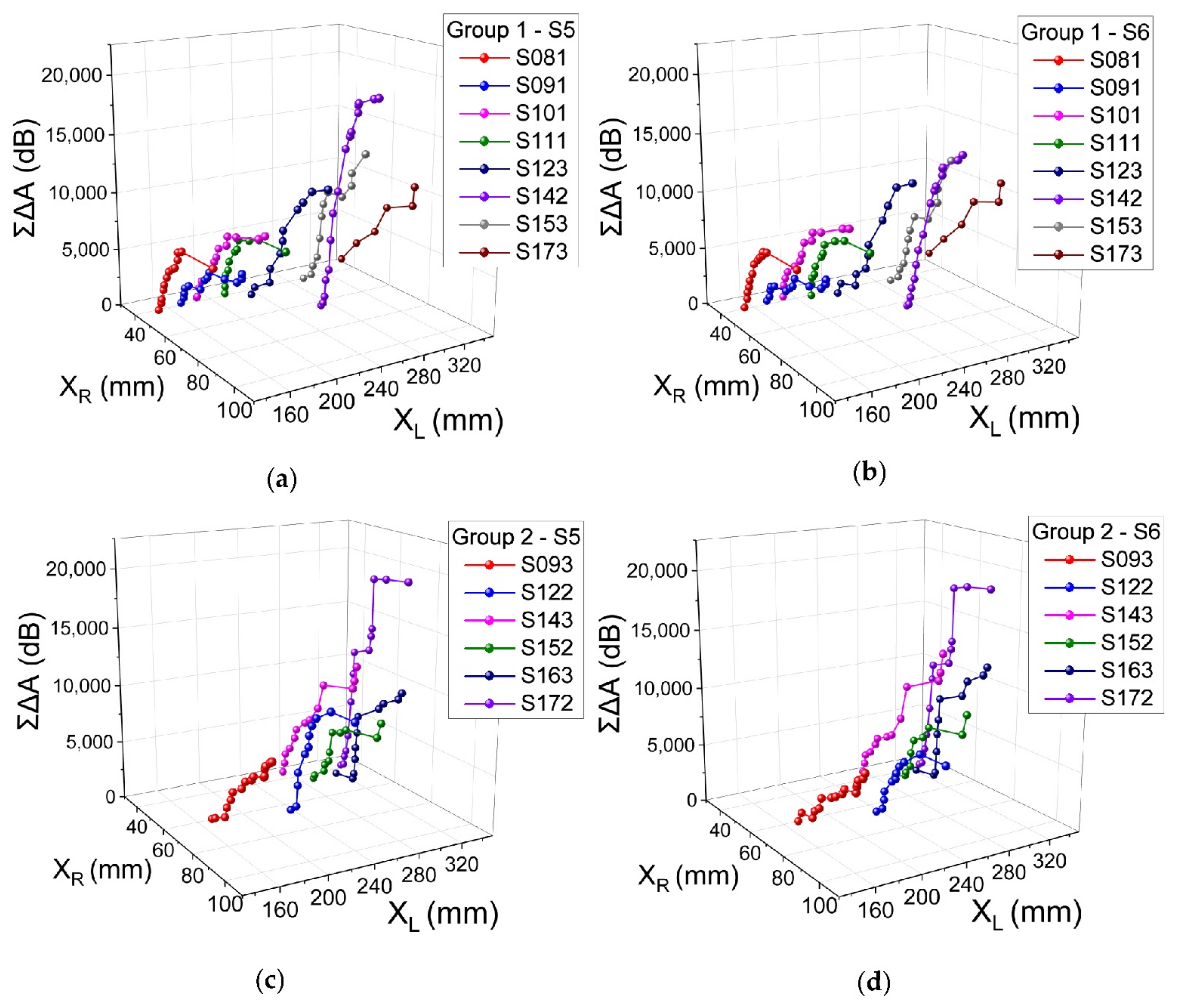
| S081, S091, S101, S111, S123, S142, S153, S173 | Group 1 | Parallel to grain | 4° | 9° |
| S093, S122, S143, S152, S163, S172 | Group 2 | Not parallel to grain | 5° | 10° |
Publisher’s Note: MDPI stays neutral with regard to jurisdictional claims in published maps and institutional affiliations. |
© 2021 by the authors. Licensee MDPI, Basel, Switzerland. This article is an open access article distributed under the terms and conditions of the Creative Commons Attribution (CC BY) license (https://creativecommons.org/licenses/by/4.0/).
Share and Cite
Bartolucci, B.; Frasca, F.; Siani, A.M.; Bertolin, C. Calibration of Acoustic Emission Parameters in Relation to the Equilibrium Moisture Content Variations in a Pinus sylvestris Beam. Appl. Sci. 2021, 11, 5236. https://doi.org/10.3390/app11115236
Bartolucci B, Frasca F, Siani AM, Bertolin C. Calibration of Acoustic Emission Parameters in Relation to the Equilibrium Moisture Content Variations in a Pinus sylvestris Beam. Applied Sciences. 2021; 11(11):5236. https://doi.org/10.3390/app11115236
Chicago/Turabian StyleBartolucci, Beatrice, Francesca Frasca, Anna Maria Siani, and Chiara Bertolin. 2021. "Calibration of Acoustic Emission Parameters in Relation to the Equilibrium Moisture Content Variations in a Pinus sylvestris Beam" Applied Sciences 11, no. 11: 5236. https://doi.org/10.3390/app11115236