CFD Assessment of the Hydrodynamic Performance of Two Impellers for a Baffled Stirred Reactor

Abstract

When converting a baffled stirred reactor to work with a different fluid, usually the original impeller must be replaced with a customized one. If the original impeller was designed for mixing liquids, its performance for liquid–solid suspensions may not be satisfactory. A case study is presented, where a two-blade original impeller is replaced with a new three-blade design. The new impeller shows clear improvements in mixing a liquid–solid suspension, while keeping the shaft power practically at the same level. As a result, a practically homogenous liquid–solid mixture is obtained, thus ensuring the required quality of the final product. The present numerical investigations employ the Eulerian multiphase model with renormalization (RNG) k–ε turbulence model to simulate the three-dimensional unsteady free-surface liquid–solid flow in a stirred tank. A sliding mesh approach was used to account for the impeller rotation within the expert code, FLUENT 16. The comparative quantitative analysis of the solid phase distribution and the relevant velocity profiles show that the new design of three-blade-impeller is significantly increasing the sedimentation time of the solid phase beyond the chemical reaction specific time. The necessary power to drive the new impeller has a slightly higher value than for the original impeller but it can be sustained by the existing driving system.

1. Introduction

Stirred reactors have applications in many chemical processes where mixing is important for the overall performance of the system. In such systems, detailed information on the fluid characteristics resulting from the effect of the reactor and impeller geometries is required [1,2,3]. Computational fluid dynamics (CFD) techniques have been used in the recent years to provide such information of the hydrodynamic and design parameters. Hydrodynamics and mixing efficiency in stirred reactors are important for the design of many industrial processes.

Due to its practical importance, the turbulent fluid flow inside stirred tanks, with various geometries and applications, has been simulated with various expert CFD codes (Fluent, CFX) [4,5,6,7,8,9]. The results obtained have shown the robustness of these codes to characterize the flow hydrodynamics in stirred tanks. The accuracy of different simulation methods (k–ε, RSM and LES) used to describe the turbulent flow has been studied [5,6]. Taking into consideration the results of the previous studies, we decided to use the RNG k–ε turbulence model, which allows sufficient accuracy of the turbulent quantities within a reasonable calculation time.

For the modelling of the solid suspension there are two models mentioned in the literature: the Eulerian multiphase model and the Eulerian mixture model. In the Eulerian multiphase model, continuity and momentum balance equations are solved for each phase. The Eulerian mixture model is a simplified version of the previous model and it is suitable for dilute suspensions and small particle Stokes number. For this model continuity and momentum balance equations are solved for one mixture phase, the hydrodynamics parameters of which are computed from mass-averaged properties of each phase. Only one equation for the transport of volume fraction is added and solved for the dispersed phase from the continuous phase. This term consists of four different interphase forces: lift force, Basset force, virtual mass force and drag force. Due to the small influence of lift, Basset and virtual mass forces on the simulated solid hold-up profile, only the drag force may be considered in the interphase momentum exchange term (Schiller–Naumann). In the literature [10,11,12,13,14], there are available results obtained from using these two models and these results show that the Eulerian multiphase model is more accurate than the Eulerian mixture model when working with a particle size higher than 100 µm and solid fraction ranging between 0.2 and 16%. The Eulerian mixture model is better adapted for low particle size and concentration.

Hoseini et al. [15] presents the analysis of the operation for different types of optimized impellers using the professional code CFX. The standard k–ε model was employed to model the turbulence together with the sliding mesh method and a residual error for all the equations set at 10⁻⁴. The numerical results were validated with experimental results. Valizadeh et al. [16] analyzed the turbulent flow of the non-Newtonian fluid with the help of the software Fluent. The k–ε model was considered for modeling the turbulence and a convergence criterion of 10⁻⁶. The distribution of the velocity and pressure was investigated inside spiral tubes and the conclusion was that the friction coefficient is higher than for the straight tube and the friction coefficient decreases while the Reynolds number increases. De Lamotte et al. [17] presents the results of CFD investigation of the hydrodynamic field of a baffled stirred tank equipped with two impellers. The professional software Ansys Fluent was employed with the realizable k–ε model for the turbulence and the volume-of-fluid method formulation for the multiphase flow. Two approaches were studied for modelling the movement of the impellers: moving reference frame and sliding mesh. The qualitative and quantitative comparison of the velocity field, obtained from numerical simulation and PIV measurements, is performed and a good overlapping is discovered.

The above brief literature review on the numerical approaches for problems similar to the one addressed in the present paper led us to the conclusion that the Eulerian multiphase model is the suitable one for the liquid–solid mixture reactor further investigated. Moreover, this model can accommodate the free-surface flow.

The current study represents the second research paper from a series of three and focuses to analyze the hydrodynamic performance of a new impeller designed by our research team, which is fitted on a stirring mechanism of a chemical reactor. In the previous research paper [18], we analyzed the performances of an impeller, which was initially designed and used for operating in a liquid–liquid environment. After analyzing the results obtained from CFD we concluded that this original impeller cannot be used in a liquid–solid phase flow because it cannot prevent the settlement of the solid particles on the bottom part of the reactor. Additionally, this impeller cannot ensure a uniform dispersion of the solid particles inside the liquid phase, an aspect that is critical for the chemical reaction that takes place inside the reactor.

A schematic representation of the investigated stirred reactor is presented in Figure 1, where the new designed impeller is fitted.

In Figure 2 the new designed impeller versus the initial one is represented: the original one that was initially fitted to the stirring mechanism of the industrial reactor, Figure 2a, and the one designed by our research team, Figure 2b. The impeller designed by our research team has a smaller diameter than the original one, the diameter of the new impeller is 1.2 m, while the diameter of the original one was 1.4 m. Additionally, the new impeller has three blades instead of two, as the original impeller had. The new designed impeller was fitted to the stirring mechanism in the same position, regarding the bottom of the reactor, as the original impeller.

After analyzing the results obtained from CFD and judging the hydrodynamic performance of the two impellers from the point of view of the dispersion of the solid phase in the entire volume of the liquid phase, a decision will be taken if the original impeller will be kept, or the new designed impeller will be better fitted to the stirring mechanism in order to ensure the prescribed solid particle distribution.

2. Materials and Methods

In this paper the Eulerian multiphase model was chosen to describe the flow behavior of each of the liquid and solid phase. This model is the most complex model and it solves a set of momentum equations for each phase.

For simulating the turbulence effects, the RNG k–ε model with the dispersed option was chosen. The dispersed turbulence model is the appropriate model when using the granular model.

Geometry reconstruction of the industrial stirred reactor fitted with the new designed impeller and its meshing were performed with the software Gambit 2.4. The mesh consists of approximately 0.6 million tetrahedral elements. As regards the mesh quality, we use tetrahedral mesh cells as recommended for such complex geometries, [2,3]. In this study a good quality of mesh (skewness < 0.96) was ensured throughout the computational domain.

As in previous research paper we used the sliding mesh approach, and four fluid zones were defined: an inner rotating cylindrical volume centered on the impeller and three other volumes containing the rest of the reactor and the baffles. The interface was located at an equal distance from the blades of the impeller and the inside edge of the baffles. An illustration of the domain and the mesh of the domain is given in Figure 3, which shows that finer meshes were used around the impeller where the velocity spatial gradients were expected to be large. Good care was taken in keeping the same mesh dimension between the rotating and the stationary interface to ensure a good exchange of the hydrodynamic quantities between the two zones during calculation. A “no-slip” condition was applied on all walls of the geometry.

Simulations of the turbulent multiphase flow were then performed with the help of the commercial CFD code Fluent 16 [19] using the RNG k–ε model. There were three working materials corresponding to the three phases: liquid with the density ρ_l = 690 kg·m⁻³, powder with the density ρ_p = 1520 kg·m⁻³ and the particle size d = 171 µm and air with the density ρ_a = 1.225 kg·m⁻³. At the liquid surface, a gas zone consisting of air was added at the free surface of water, a method that was reported to dampen the instabilities, which means top surface being exposed to atmospheric pressure.

The limitations of the k–ε turbulence models in predicting the dissipation rate and the power number are well known [5,17] and also the numerical results depend on the limitation of the model employed for modeling the impeller rotation. Our analysis was centered on the prediction of the flow field inside the reactor in order to assess the performances of the original impeller. For this purpose, the accuracy of the turbulence model that was employed is satisfactory, as stated by previous research [5,6,8,17,20].

Using the sliding mesh approach, the flow resolution is unsteady. At each time step, the position of the rotating zone relative to the stationary one was recomputed and the grid interface of the rotating zone slides along the interface of the stationary zone. For all simulations, the time step was set as a function of the impeller speed, 65 rot/min, and the number of the cells from the interface surface, approximately 140 elements, so that the time step was set to a value of 0.01 s.

At the end of each time step, after a maximum of 5 iterations, the convergence criterion reaches 10⁻³ for the continuity, for momentum and turbulence quantities. Simulations were performed in double precision with the segregated implicit solver. Transient formulation is of the second order and spatial discretization scheme for pressure is PRESTO! and for momentum and turbulence is QUICK. The SIMPLE algorithm has been employed for the pressure–velocity coupling [21,22,23,24,25].

The analysis of the results was performed after a total flow time of 90 s.

3. Results and Discussion

The performance of the stirring mechanism from an industrial reactor was judged from the point of view of the suspension of the entire solid phase, in a homogeneous manner, in the entire volume of the liquid phase, for as long as needed for the chemical reaction to take part. Some processes require that the particles be just suspended off the bottom, whilst, in some other processes, complete off-bottom solids suspension is necessary. To analyze the suspension of the solid phase, the distribution of the volume fraction of the solid phase was plotted on a vertical plane through the middle part of the reactor. The most relevant quantitative representation for the analysis of the performance of the stirring mechanism is represented by the histogram of the distribution of the volume fraction of the solid phase. A similar investigation of the distribution of the solid phase was presented by Gohel et al. [3], in order to analyze the performance of the stirring mechanism.

Liquid velocities distributions also provide an insight into the mixing process occurring inside stirred reactors. The velocity components (axial, radial and tangential) are plotted on a vertical midplane and the velocity components radial distribution is presented for three sections corresponding to the impeller level (i0), above impeller (i+) and below the impeller (i-).

The two cases investigated correspond to the original impeller and the new one designed by our research team. For both cases, the initial state of the flow corresponds to the homogeneous distribution of the volume fraction of the solid phase in the entire volume of liquid. This is the most favorable situation for the best operation of the reactor as it resulted from our previous research work.

From analyzing Figure 4, it results that the new impeller was performing better than the original one. The volume fraction of the liquid containing no solid particles decreased from 25% to 20% as shown by the histograms. Additionally, the new impeller completely prevented the sedimentation of the solid phase on the lower part of the reactor as can be seen from the distribution of the volume fraction of the solid phase on the vertical plane and from the histogram, Figure 4b.

To underline the better performance of the new impeller regarding the original one, the distribution of the velocity components was analyzed. A similar representation of the velocity field, employed for analyzing the hydrodynamic performance of the impeller and also to validate the numerical results, are presented in previous research papers [3,5,6,7,8,17].

From analyzing the distribution of the axial velocity on a vertical plane, Figure 5, and on three horizontal sections, Figure 6, it resulted that the new impeller generated a larger value for the axial component of the velocity, pointing to the bottom of the reactor. The new impeller generated, in the middle part, a downward jet below the impeller, that kept the entire volume fraction of the solid phase in suspension. Then the axial velocity was decreasing and the flow turned upwards near the walls of the reactor.

The axial component of the velocity generated by the original impeller had smaller values for all the investigated sections. Moreover, in the section below the impeller (i0), Figure 6c, the value of the axial component was almost zero for the entire section and this explains the poor operation of the impeller, leading to the sedimentation of the solid phase on the bottom of the reactor.

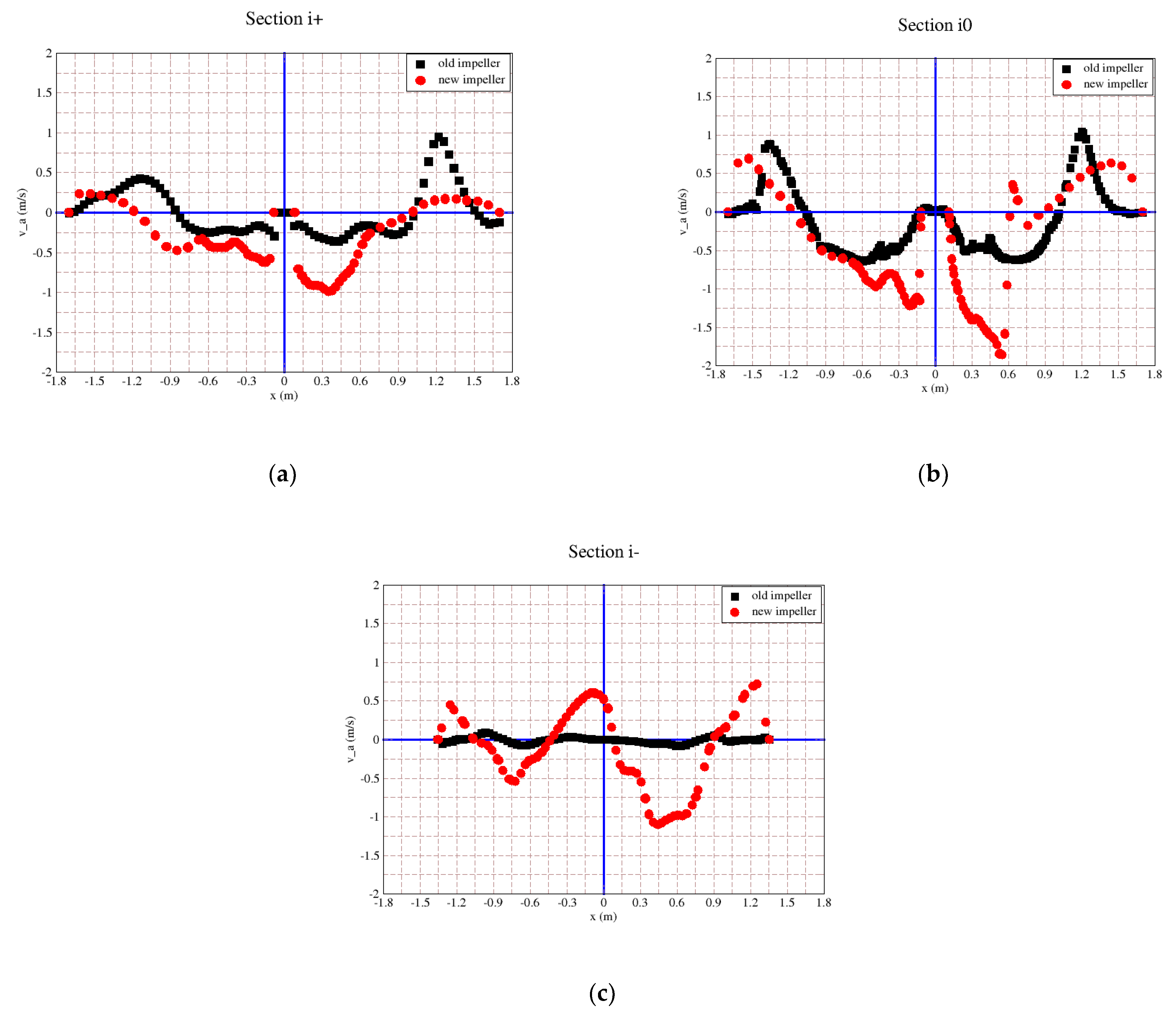
The comparison of the radial profiles of the radial velocity is shown in Figure 7 and Figure 8. For the new impeller, in the impeller centre plane (i0), Figure 8b, the radial flow increased gradually from the wall and a maximum occurred near the impeller blade tip. Radial profile of the radial velocity below the impeller (i-), Figure 8c, show that, the radial flow was towards the wall of the reactor and the velocity increased right from the axis and attained a maximum. After attaining the maximum value, radial velocity decreased and became small near the wall.

From Figure 8 it resulted that the radial component of the velocity generated by the original impeller had lower values than the new designed impeller for all three investigated sections.

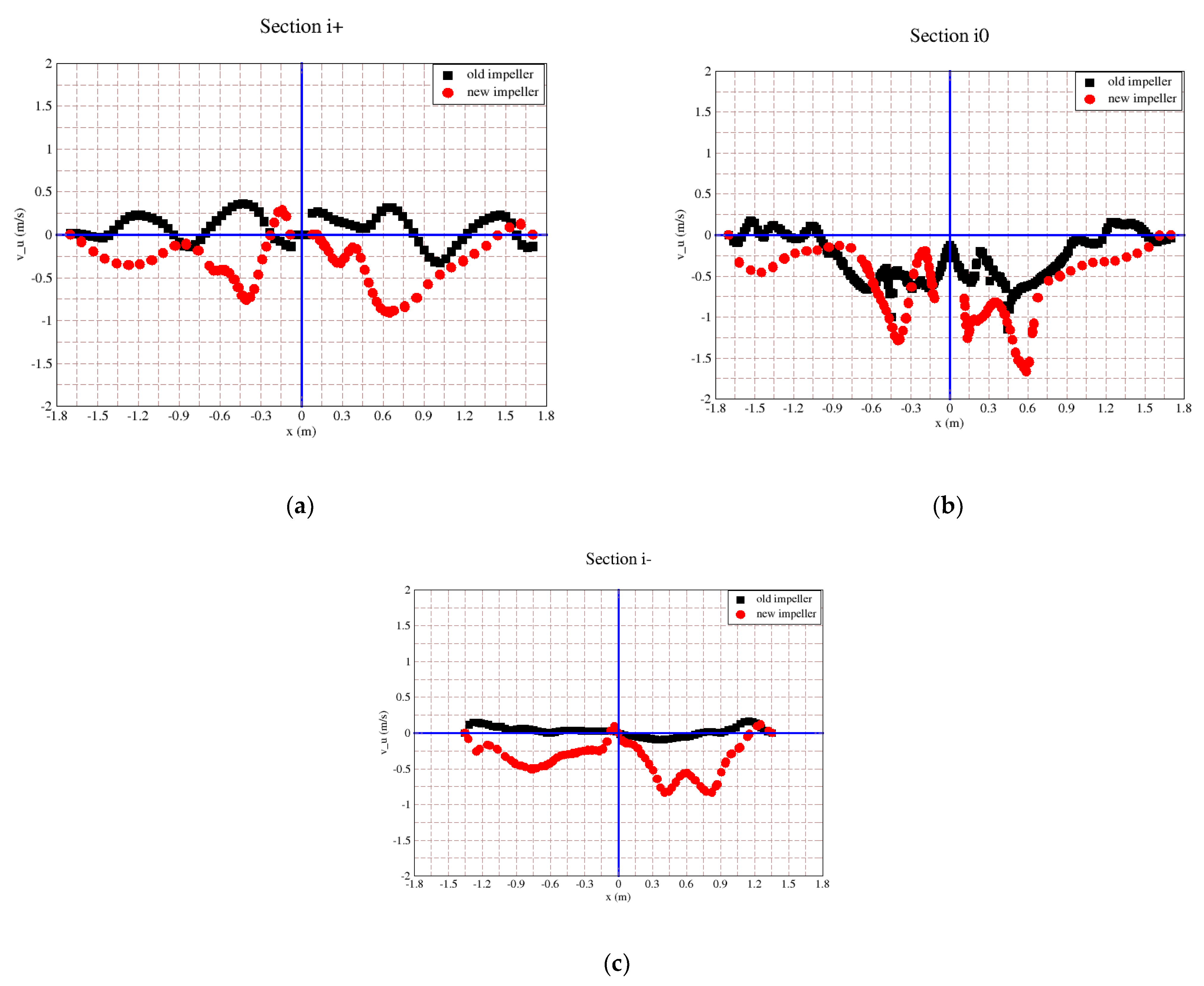
Figure 9 and Figure 10 show the tangential velocity comparation. It can be noticed that the tangential flow for the new impeller was in the direction of the impeller rotation at all the axial levels, Figure 10. For the new impeller, the value of the tangential velocity increased and decreased steeply as going from the axis towards the tip of the blades. The maximum velocity was comparable with the maximum axial velocity at all the levels.

From Figure 10c it resulted that below the original impeller the tangential velocity component had a value close to zero across the entire section. This also explains the poor operation of the original impeller fitted to the stirring mechanism.

Analyzing the flow field generated by the original impeller it can be observed, from Figure 6c, Figure 8c and Figure 10c, that dead zones exist right below the impeller and that is the reason why the original impeller did not prevent the sedimentation of the solid particles.

From the analysis of the velocity components distribution, it resulted that the new impeller generated a much stronger mixed axial–radial flow than the original impeller. This flow pattern developed by the new impeller has the form of a jet, which spreads radially as it progresses towards the base of the reactor, entraining liquid adjacent to the impeller. After hitting the bottom wall of the reactor, part of the axial momentum gets converted to the radial component along the base towards the side walls of the reactor. Due to this flow pattern, with no dead zones, there was no sedimentation of the solid phase when the new impeller was operating.

A calculation was performed to check if the existing electrical motor, which drives the stirring mechanism, can provide sufficient power for the new impeller. The electrical motor generated a power of 3.6 kW and the power needed by the new impeller to operate had the value of 2.32 kW. It resulted that the existing electrical motor can be used to drive the stirring mechanism fitted with the new impeller, so no supplementary cost was generated. To compare the performances of the two impellers from the point of view of consumption of power is recommended to calculate the power number, N_P, with the following equation [15,17]:

$$N_P=\frac{P}{{\rho }_l\cdot n^3\cdot d^5}$$

(1)

The value of the power number for the original impeller was 0.43 and for the new designed impeller it was 1.06. Although the power number for the new designed impeller was higher than the original impeller, the hydrodynamic performances were superior.

Although it was performing better than the original impeller, the new impeller was not operating at its best, because there was still a consistent volume of liquid, 20%, with no solid particles in it. This means that the part of the volume of liquid with no solid particles in it will be wasted, because no chemical reaction will take part in that region of the reactor.

4. Conclusions

In this paper we present the results of the CFD analysis of the hydrodynamic performances for two different impellers for an industrial reactor. For the numerical analysis of the flow inside the reactor, we employed the professional software Fluent 16 with the Eulerian multiphase model for modeling the two-phase liquid–solid with the free surface flow and the RNG k–ε model for turbulence. The sliding mesh approach was employed for modeling the rotation of the impeller.

Two cases were analyzed: the original two-blade impeller and the new three-blade impeller designed by our research team. The two impellers started to operate when the solid phase was initially homogenously distributed in the entire volume of liquid. The quantitative assessment of the performance of the two impellers employed the distribution of the volume fraction of the solid phase in the bulk flow and the histogram of the solid fraction after 90 s of flow time. A further detailed explanation of the result is based on the velocity field analysis in a meridian plane and in horizontal cross sections above the impeller, at the same impeller level and below the impeller.

From the analysis of the distribution of the solid phase volume fraction one can immediately conclude that the new three-blade impeller provides a practically homogenous liquid–solid suspension while the original two-blade one led to significant sedimentation. The better performance of the new impeller was due to the generated axial–radial flow pattern. Another finding is that the electrical motor that drives the stirring mechanism could be kept driving the new impeller without additional cost.

Further improvements of the three-blade design were still possible and necessary since approximately 20% percentage of liquid phase on top of the reactor was still depleted of solid particles.