Reduction of Annual Operational Costs in Power Systems through the Optimal Siting and Sizing of STATCOMs

Abstract

The problem of the optimal siting and placement of static compensates (STATCOMs) in power systems is addressed in this paper from an exact mathematical optimization point of view. A mixed-integer nonlinear programming model to present the problem was developed with the aim of minimizing the annual operating costs of the power system, which is the sum of the costs of the energy losses and of the installation of the STATCOMs. The optimization model has constraints regarding the active and reactive power balance equations and those associated with the devices’ capabilities, among others. To characterize the electrical behavior of the power system, different load profiles such as residential, industrial, and commercial are considered for a period of 24 h of operation. The solution of the proposed model is reached with the general algebraic modeling system optimization package. The numerical results indicate the positive effect of the dynamic reactive power injections in the power systems on annual operating cost reduction. A Pareto front was built to present the multi-objective behavior of the studied problem when compared to investment and operative costs. The complete numerical validations are made in the IEEE 24-, IEEE 33-, and IEEE 69-bus systems, respectively.

1. Introduction

Electricity is considered around the world as a public and essential service, which has the potential to improve the quality of life of millions [1,2]; in addition, this service has driven the economic and industrial development from the end of the nineteenth century to the current times. Electricity service includes four main sub-systems: (i) generation; (ii) transmission and sub-transmission; (iii) distribution; and (iv) commercialization [3]. All of these components are essential for transferring electricity from power plants to end-users [4,5]. Two important worldwide issues correspond to the harmful effects of thermal generation on the atmosphere and the efficiency of the entire system. The former problem of modern power systems can be solved with the inclusion of renewable energy resources, mainly from photovoltaic and wind generation plants, which are now mature generation technologies [6] and can thus help with the continuous replacement of fossil fuels in conventional thermal systems. The latter problem regarding system efficiency is independent of the generation technology and is associated with the physical characteristics of the power system elements (generators, lines, transformers, etc), which produce energy losses, i.e., electrical energy that is dissipated in the form of heat by the resistive effects of mainly the transmission and transformers [7]. In the Colombian context, the amount of power losses in the power system (lines with voltages $\ge 220$ kV) is between $1.5\%$ and $2.0\%$ of the energy generated, which implies that, for a peak load scenario, the total power loss oscillates between 141 and 188 MW [8].

To minimize power losses in the electrical power systems, different methodologies are used, such as optimal reactive power dispatch [9,10], optimal integration of dynamic reactive power compensators [11,12], and optimal integration of battery energy storage systems [13,14,15]. Of the aforementioned methodologies, the literature considers the first two as being more effective in minimizing the losses of the power systems [16] and batteries as being more suitable to help with the integration of renewable energy resources to mitigate their dependence on weather conditions [17,18].

The dynamic reactive power compensation is an excellent alternative for helping with the energy losses problem in transmission and distribution networks [12,19], as the devices used for this purpose, i.e., STATCOMs, have long useful-life, low investments and maintenance costs, and high reliability [20]. In the literature, multiple approaches have been proposed for integrating STATCOMs in power systems. Some of them are as follows: Abd-Elazim and Ali [21] proposed the cuckoo search algorithm to locate and size STATCOMs in multi-machine power systems to increase the system loadability. Numerical results demonstrate the superiority of the proposed cuckoo search algorithm when compared to the classical genetic algorithm and the heuristic open loop method. Dutta et al. [22] studied the problem of the optimal siting and sizing of STATCOMs for solving the optimal reactive power flow problem in power systems by implementing the chemical reaction optimization method. Numerical simulations in the IEEE 30- and IEEE 57-bus systems demonstrate the effectiveness of the proposed method regarding total power losses value when compared with classical approaches reported in the literature such as the particle swarm optimizer and differential evolution method. The authors of [23] proposed an improved version of the particle swarm optimizer to locate and size STATCOMs in power systems with photovoltaic sources to minimize the costs of the energy losses and the voltage profile improvement. Numerical results demonstrate the effectiveness of the proposed approach in comparison with the bee colony optimization and the lightening search algorithm, respectively. The following are some additional approaches for locating and sizing STATCOMs in power and distribution networks: the tabu search algorithm [24], bat optimization algorithm [25], discrete-continuous vortex search algorithm [16], genetic algorithms [26,27], and firefly optimization algorithm [28].

To deal with the problem of power losses minimization in power systems, we propose a mixed-integer nonlinear programming model (MINLP) for optimally locating and sizing STATCOMs in power systems considering different load scenarios (commercial, residential, and industrial) [11]. The aim of the proposed (MINLP) model is to reduce the annual operative cost of the power system. This objective function is composed by the costs of the energy losses during the planning horizon and the installation costs of the STATCOMs. The general algebraic modeling system (GAMS) software with the BONMIN large-scale optimization solver is used to solve the MINLP model; this software was selected as a optimization tool due to the excellent reports presented in the literature for similar MINLP models [29,30]. The main contributions of our approach are summarized below:

• To formulate the problem of the optimal siting and sizing of STATCOMs in power systems as a multi-objective optimization problem, where the objective functions in conflict are the cost of annual energy losses and the investments in STATCOM devices.
• The solution of the single-objective model and the multi-objective model using the GAMS software and BONMIN, where it was observed that the minimum solution in the Pareto front regarding the total annual operative costs of the network after the installation of the STATCOMs differs by only $0.02$% with respect to the single-objective model.
• The application of the solution methodology to radial and meshed power systems in high- and medium-voltage levels combined with residential, industrial, and commercial load curves to characterize the behavior of the constant power consumption.

It is important to highlight that the proposed optimization methodology with the GAMS optimization package and the BONMIN solver has not been previously reported in specialized literature on radial and meshed power systems with multiple generators considering different load curves; this scenario of optimization was identified as an opportunity of research that this work endeavors to fill. In the recent literature, two works on the optimal installation of STATCOMs in distribution systems have been presented. An algorithm-denominated discrete-continuous vortex search algorithm was proposed by Montoya et al. [16] to locate and size STATCOMs in distribution grids with fast convergence and solution repeatability; however, this approach is only applicable to distribution grids with radial or meshed configuration that have only one slack source without voltage controlled nodes, which makes it impossible to extend it to high-voltage power systems with multiple generators. The authors of [11] presented a hybrid optimization approach based on the classical Chu and Beasley genetic algorithm and the conic reformulation of the optimal power flow equations; however, the conic reformulation is only applicable to pure radial distribution grids with only one slack source, which makes this approach non-applicable to power systems in high-voltage levels. Note that, due to the limitations of the previous approaches regarding transmission power systems, here, we adopt the GAMS optimization package and the BONMIN solver to solve the problem of the optimal placement and sizing of STATCOMs in electrical networks independent of the grid configuration, i.e., radial or meshed or with multiple generation sources. This can be considered as one of the main contributions of this work.

Note that the contribution of this research is focused on proposing an exact MINLP to represent the problem of the optimal siting and sizing of STATCOMs in power systems operated with high- and medium-voltages, i.e., transmission meshed networks and radial distribution ones with a unique and reliable optimization model. This implies that the usage of the GAMS software and the BONMIN package is not the sole contribution. However, these tools allow one to focus on the mathematical formulation, not the optimization method as is recurrently done in the literature when metaheuristic methods are proposed. This is an advantage when the interest is to provide efficient and accurate optimization models for engineering problems.

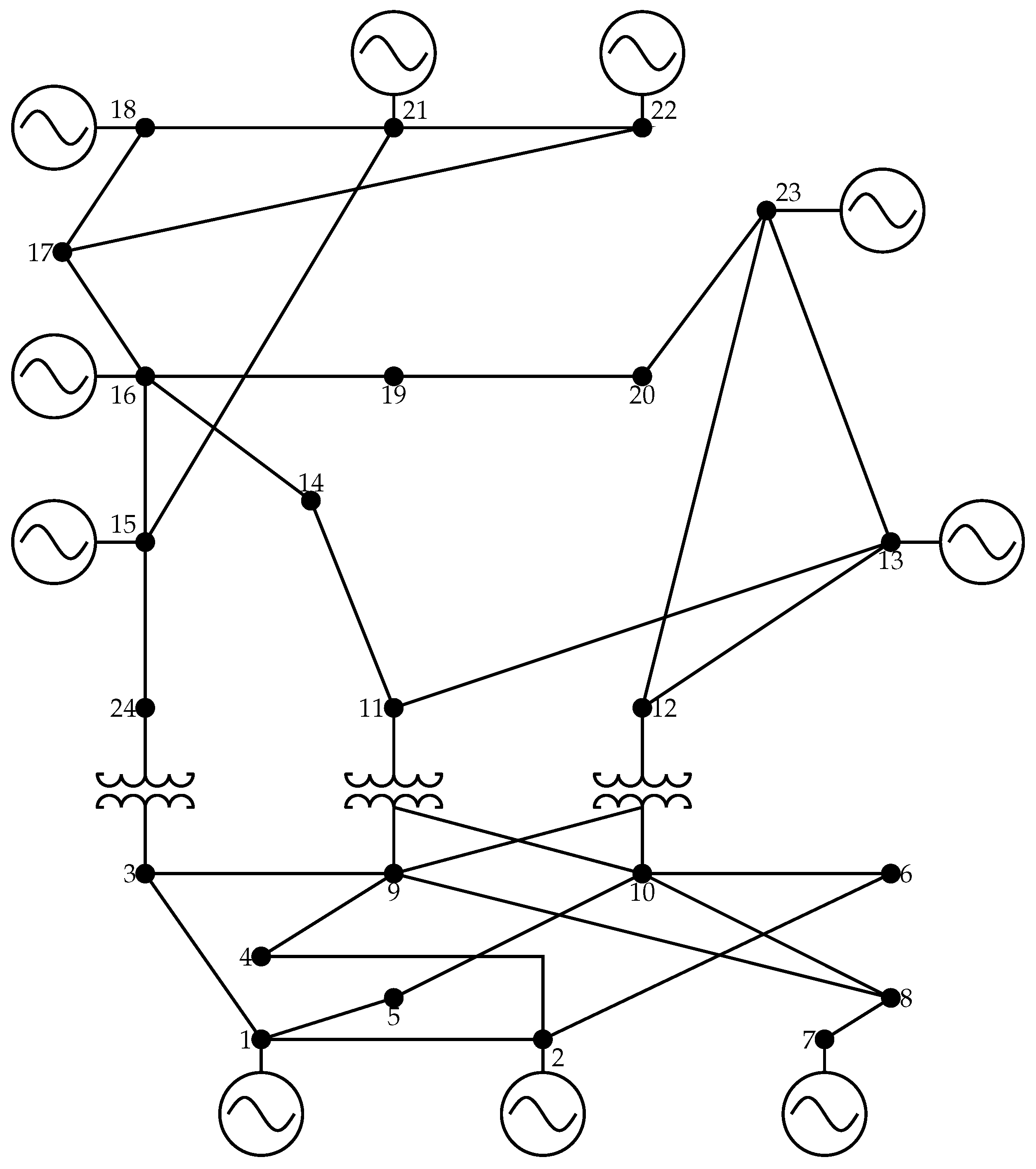
The remainder of this manuscript is structured as follows. Section 2 presents the MINLP formulation for the problem of the optimal siting and sizing of STATCOMs in power systems. Section 3 presents the main aspects of the solution methodology based on the GAMS optimization tool. Section 4 shows the main characteristics of the test systems composed of 14 and 30 nodes. Section 5 describes the main numerical results and analyzes and discusses them. Section 6 presents the conclusions derived from this study.

2. Mathematical Optimization Model

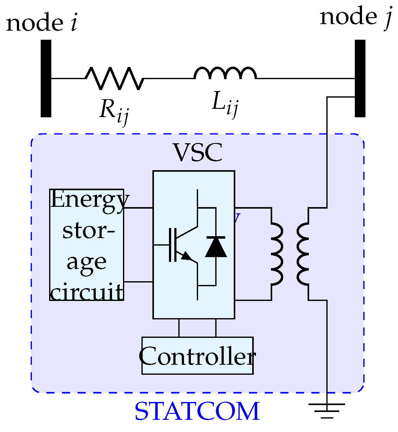
To understand how a STATCOM-supplied reactive power is formed into electrical grids, consider the schematic representation of a STATCOM presented in Figure 1. In this representation, we observe that the STATCOM is a device composed of a power electronic converter and a small energy storage device (battery or capacitor) that is connected to the grid using a transformer [12]. The connection of the STATCOM is shunt, and the possibility of dynamically controlling the reactive power with lagging or leading power factors is dependent on the converter and the linear/nonlinear control technique applied on it [31].

In the following optimization model, we assume that the controller is applied on the STATCOM to reach the desired reactive power output (i.e., the reference). In this sense, the proposed optimization model to site and size STATCOMs in power systems can be considered as the tertiary control scheme, as, once the location of the STATCOMs is defined, the optimization model defines the desired reactive power curve that each STATCOM must follow to minimize the total grid energy losses. The complete optimization model is formulated below.

2.1. Objective Function Formulation

The objective function for the problem of the optimal placement and sizing of STATCOMs in power systems corresponds to the minimization of the annual operating costs related to the cost of energy losses and the installation of the STATCOMs, respectively. These components of the objective function are defined in Equation (1).

$$\begin{array}{c}\hfill min{A}_{\cos \mathrm{t}}=f_1+f_2,\\ \hfill f_1=C_{\mathrm{kWh}}T\sum _{h\in \mathcal{H}}\sum _{k\in \mathcal{N}}\sum _{m\in \mathcal{N}}{Y}_{km}{V}_{kh}{V}_{mh}cos\left({\delta }_{kh}-{\delta }_{mh}-{\theta }_{km}\right){\Delta }_h,\\ \hfill f_2=T\left(\frac{k_1}{k_2}\right)\sum _{k\in \mathcal{N}}\left(\alpha {\left(y_k\right)}^2+\beta y_k+\gamma \right)y_k,\end{array}$$

(1)

where $f_1$ is the component of the objective function associated with the annual operative costs produced by the energy losses; $f_2$ represents the annualized investment costs in STATCOMs; $A_{\cos \mathrm{t}}$ represents the objective function value associated with the linear combination of the components $f_1$ and $f_2$, i.e., the total annual operating costs of the power system; $C_{\mathrm{kWh}}$ corresponds to the average cost of electric energy; T represents the plan horizon period (i.e., 365 days); and $Y_{km}$ and ${\theta }_{km}$ are the magnitude and angle of the admittance that relates nodes k and m, respectively. $V_{kh}$, $V_{mh}$, ${\delta }_{kh}$, and ${\delta }_{mh}$ represent the voltage magnitudes and angles associated with buses k and m, respectively, in the period h. ${\Delta }_h$ represents the length of the period of time where the loads are constant, i.e., 1 h in this research, and $k_1$ and $k_2$ correspond to positive constants associated with the installation costs of STATCOMs. $\alpha$, $\beta$, and $\gamma$ are positive constants related with the variable costs of the STATCOMs (costs associated with the reactive power injection of the STATCOMs i.e., $y_k$). Note that $\mathcal{H}$ and $\mathcal{N}$ represent the sets that have all the periods of time and buses of the network, respectively.

Remark 1.

Note that the structure of Equation (1) corresponds to a single-objective optimization problem. In the case of multi-objective optimization, the structure of the objective functions is the following:

$$\begin{array}{c}\hfill min{f}_1=C_{\mathrm{kWh}}T\sum _{h\in \mathcal{H}}\sum _{k\in \mathcal{N}}\sum _{m\in \mathcal{N}}{Y}_{km}{V}_{kh}{V}_{mh}cos\left({\delta }_{kh}-{\delta }_{mh}-{\theta }_{km}\right){\Delta }_h,\\ \hfill min{f}_2=T\left(\frac{k_1}{k_2}\right)\sum _{k\in \mathcal{N}}\left(\alpha {\left(y_k\right)}^2+\beta y_k+\gamma \right)y_k.\end{array}$$

Note that the goal of the multi-objective model corresponds to the minimization of both objective functions due to the nature of these that correspond to the investment and operating costs, which ideally must tend toward zero.

2.2. Set of Constraints

The restrictions of the problem of the optimal placement and sizing of STATCOMs in power systems are associated with classical power flow constraints, voltage regulation bounds, and devices’ capabilities. These constraints are presented below.

$$\begin{array}{c}\hfill P_{kh}^g-P_{kh}^d=\sum _{k\in \mathcal{N}}\sum _{m\in \mathcal{N}}{Y}_{km}{V}_{kh}{V}_{mh}cos\left({\delta }_{kh}-{\delta }_{mh}-{\theta }_{km}\right),\forall \left\{k\in \mathcal{N}\&h\in \mathcal{H}\right\},\end{array}$$

(2)

$$\begin{array}{c}\hfill Q_{kh}^g+Q_{kh}^{\mathrm{STATCOM}}-Q_{kh}^d=\sum _{k\in \mathcal{N}}\sum _{m\in \mathcal{N}}{Y}_{km}{V}_{kh}{V}_{mh}sin\left({\delta }_{kh}-{\delta }_{mh}-{\theta }_{km}\right),\forall \left\{k\in \mathcal{N}\&h\in \mathcal{H}\right\},\end{array}$$

(3)

$$\begin{array}{c}\hfill V_{min}\le V_{kh}\le V_{max},\forall \left\{k\in \mathcal{N}\&h\in \mathcal{H}\right\},\end{array}$$

(4)

$$\begin{array}{c}\hfill x_k{Q}_{min}^{\mathrm{STATCOM}}\le y_k\le x_k{Q}_{max}^{\mathrm{STATCOM}},\forall \left\{k\in \mathcal{N}\right\},\end{array}$$

(5)

$$\begin{array}{c}\hfill -y_k\le Q_k^{\mathrm{STATCOM}}\le y_k,\forall \left\{k\in \mathcal{N}\&h\in \mathcal{H}\right\},\end{array}$$

(6)

$$\begin{array}{c}\hfill \sum _{k\in \mathcal{N}}{z}_k\le N_{\mathrm{available}}^{\mathrm{STATCOM}},\end{array}$$

(7)

Note that $P_{kh}^g$ and $Q_{kh}^g$ correspond to the active and reactive power injection associated with the generators connected at node i during the period h, while $P_{kh}^d$ and $Q_{kh}^d$ are the active and reactive consumptions at node i during the period h. $V_{min}$ and $V_{max}$ represent the minimum and maximum voltage limits allowed for all buses of the system for each period of time and $y_k$ represents the continuous variable associated with the size of the STATCOM connected at node k. $Q_{min}^{\mathrm{STATCOM}}$ and $Q_{max}^{\mathrm{STATCOM}}$ represent the lower and upper sizes of the STATCOMs that can be installed in the power system. $z_k$ is a binary variable regarding the installation ($z_k=1$ or $z_k=0$) of a STATCOM in the power system and $N_{\mathrm{available}}^{\mathrm{STATCOM}}$ corresponds to the number of STATCOMs available for installation in the power system.

Remark 2.

The optimization model defined in (1)–(7) is based on the formulation proposed in [16]. However, a new constraint was added to ensure that the STATCOM can inject variable reactive power into the power system as a function of its daily performance.

It is important to highlight that Montoya et al. [16] presented an optimization model to locate and size STATCOMs in distribution networks considering that, during the operation period (a daily demand case), the injection of the reactive power is constant in all the times, i.e., the STATCOMs work as capacitor banks. After this optimization process, an additional operative scenario is evaluated to determine the daily reactive power injection performance of the STATCOMs. However, in the optimization model proposed in this study, the variations in the reactive power injection from the STATCOMs is directly included in the power balance equations, which corresponds to an integrated optimization methodology. This differentiates it from the sequential approach reported in [16].

2.3. Interpretation of the Mathematical Model

The optimization model (1)–(7) that represents the problem of the optimal siting and sizing STATCOMs in power systems independent of the grid topology (i.e., radial or meshed with multiple generators) is interpreted in the following manner: Equation (1) corresponds to the objective function for the annual operating costs of the power systems incurred with the minimization of the cost of the energy losses and investment. Note that the problem can be solved using a single-objective function, i.e., $A_{\cos \mathrm{t}}$, or a multi-objective approach by minimizing $f_1$ and $f_2$ simultaneously. Equations (2) and (3) represent the most complicated constraints of the optimization model, as these are equality constraints related with the active power balance equations in all the nodes of the system for all periods of time. These constraints are complicating, as they are non-affine and non-convex due to the products of the voltages and trigonometric functions. The box-type constraint (4) ensures that the voltage profile performance of the grid fulfills the voltage regulation bounds demanded by regulatory entities (in Colombia, these bounds are typically ±10% for transmission and distribution grids). Restriction (5) determines the maximum size of the STATCOM that can be installed at node k if the binary variable $x_k$ is activated. The box-type constraint (6) guarantees that the reactive power provided by the STATCOM can be capacitive or inductive between its nominal rates as a function of the grid requirements for each period of time. Finally, the inequality constraint (7) bounds the number of STATCOMs that can be installed inside power system.

Remark 3.

The mathematical optimization model (1)–(7) exhibits an MINLP structure based on the existence of binary variables with regard to the siting of the STATCOMs in a power system. These are added with the continuous variables associated with active and reactive power generation, voltage magnitudes, and angles, respectively. The nonlinear structure is identified in the presence of sine and cosine functions as well as products of voltage magnitudes in constraints (2) and (3).

Based on the complex MINLP structure exhibited by the optimization model (1)–(7), in this paper, the GAMS optimization package is adopted to solve this model, with the main advantage being that the computational effort is minimum (in the order of seconds) with the possibility of being applicable to high- and medium-voltage networks.

3. Solution Methodology

To solve the MINLP model (1)–(7) and define the optimal location and sizing of STATCOMs in power systems, the GAMS software was employed. This is an optimization tool to solve large-scale optimization problems from linear programming to MINLP models, among others. The main advantage of using GAMS to solve optimization problems is the possibility of separating the solution technique from the mathematical modeling, which helps concentrating efforts for proposing a mathematical model that adequately represents the studied problem.

Table 1. Different optimization models solved using the GAMS optimization package.

Problem	Model Type	Ref.	Year
Optimal design of osmotic power plants	NLP	[30]	2015
Optimal location and sizing of batteries in power systems	MINLP	[29]	2017
A mixed-integer linear model for thermal generating units in the economic dispatch	MILP	[32]	2018
Integrated transmission and generation expansion planning considering safety constraints	MILP	[33]	2018
Design of optimal mixtures from atom groups	MILP	[34]	2018
Optimal allocation model of water resources	MINLP	[35]	2019
Optimal power flow studies	NLP	[36]	2019
Parameter estimation in single-phase transformers	NLP	[37]	2020
Optimal location and sizing of distributed generators in distribution networks	MINLP	[38]	2020
Multi-objective electric vehicles scheduling	NLP	[39]	2020
Optimal selection of calibers of conductors in DC radial distribution networks	MINLP	[40]	2021
Multi-objective operation of batteries in AC distribution networks	NLP	[41]	2021

presents a lists of different optimization problems solved with the GAMS optimization package.

In Table 1, it is possible to observe that the GAMS optimization package is suitable for solving different optimization problems such as the non-linear programming (NLP), mixed-integer linear programming models (MILP), and MINLP models, respectively.

The main aspects of the implementation of an optimization model in the GAMS package are listed as follows [42]:

✓

Definition of the sets (nodes and periods of time), tables, parameters, and scalars (i.e., nodal admittance matrix, demands, costs, etc.).

✓

Definition of the continuous and discrete variables, i.e., nodal voltages and angles, active and reactive powers, among others.

✓

Selection of the equations’ names and writing all these (optimization models (1)–(7)) using the symbolic structure of the GAMS software [29].

✓

Selection of the model type and the direction of optimization, i.e., minimization.

✓

Solution of the model using an adequate solver for MINLP problems.

Note that the main requirement is associated with an implementation in GAMS, that is, the mathematical formulation, as these must be consistent and faithfully represent the studied problem with a feasible solution space.

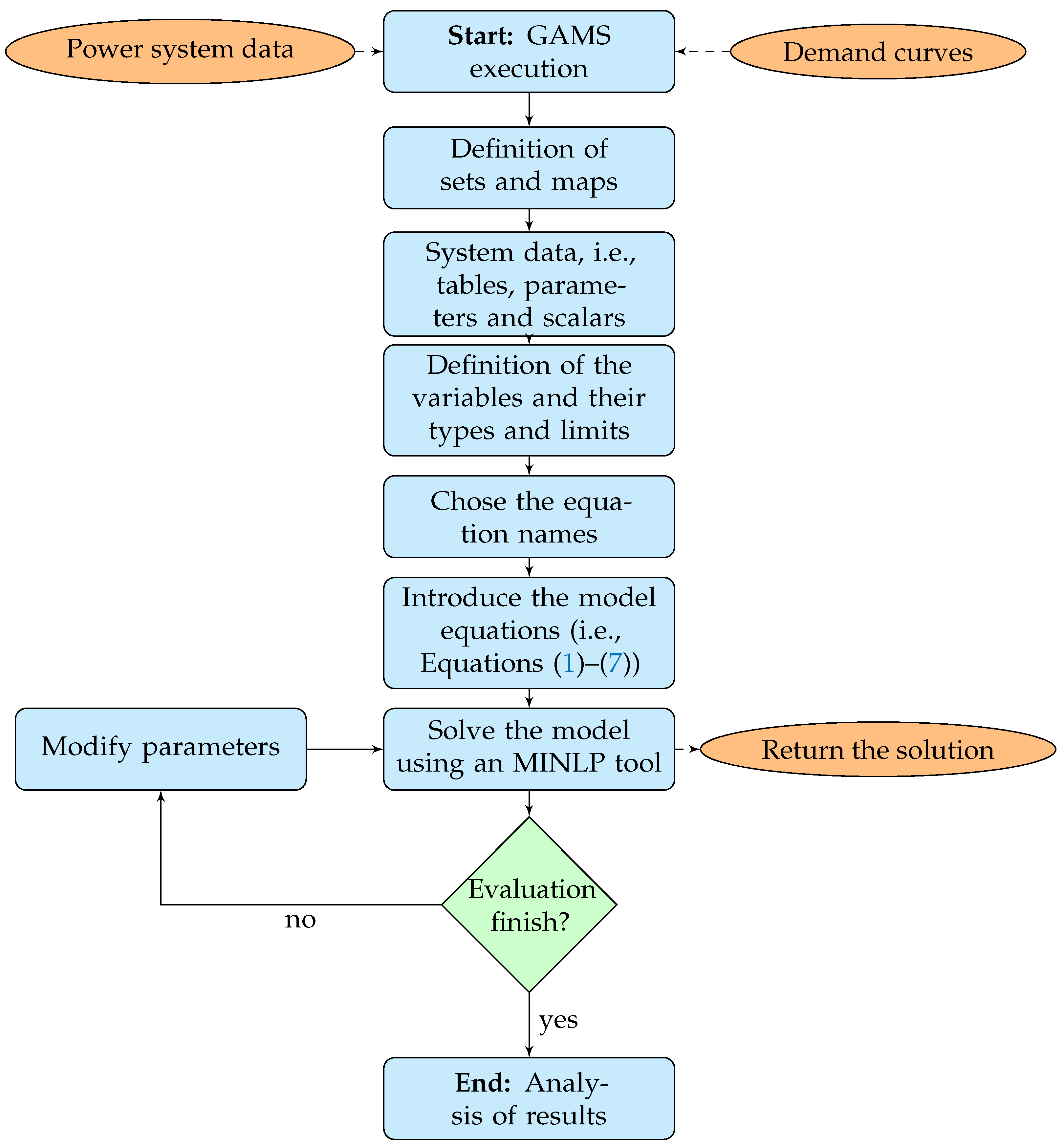
To summarize the optimization methodology, in the flow-chart presented in Figure 2, the sequential steps for implementing any optimization model using the GAMS optimization package are provided.

It is important to mention that the flow diagram presented in Figure 2 is a general procedure for solving different optimization models with the help of the GAMS software, and it only requires basic programming skills using a structured programming language. For more details regarding GAMS implementations, see the works of Soroudi [29] and Allen [43].

4. Electric Power Systems

To verify the effects of the optimal location and sizing of STATCOMs in power systems for minimizing the annual operative costs of the power system (which are associated with the costs of the energy losses and the investments costs of STATCOMs), we here consider a meshed power system composed of 24 nodes [29], and two radial test feeders composed of 33 and 69 nodes.

The main details of the IEEE-bus systems as well as the residential, industrial, and commercial load profiles for characterizing the load profiles are presented below.

4.1. IEEE 24-Bus System

This power system is composed of 24 nodes and 38 interconnections between transmission lines and transformers [29], with total active and reactive power demands in the peak load case of 2850 MW and 580 MVAr, respectively. The configuration of the IEEE 24-bus system is depicted in Figure 3. In addition, all its parametric information is reported in

Table 2. Active and reactive power capabilities in the conventional sources.

Node	${\mathit{P}}_{\mathit{g}}^{min}$	${\mathit{P}}_{\mathit{g}}^{min}$	${\mathit{Q}}_{\mathit{g}}^{min}$	${\mathit{Q}}_{\mathit{g}}^{max}$	Node	${\mathit{P}}_{\mathit{g}}^{min}$	${\mathit{P}}_{\mathit{g}}^{min}$	${\mathit{Q}}_{\mathit{g}}^{min}$	${\mathit{Q}}_{\mathit{g}}^{max}$
1	0.500	2.500	−0.750	0.750	16	0.150	1.350	−0.500	0.750
2	0.250	1.850	−0.900	0.700	16	0.150	1.350	−0.500	0.750
7	0.400	3.000	−0.800	1.200	18	0.500	4.000	−1.850	2.000
13	0.000	6.000	−5.000	5.000	21	0.450	4.500	−1.500	1.500
14	0.000	0.000	−1.500	1.500	22	0.250	2.800	−1.000	1.000
15	0.250	1.500	−0.750	0.800	23	0.750	6.000	−1.650	1.750

All data is per unit.

,

Table 3. Power consumption in the demand nodes for the IEEE 24-bus system.

Node	${\mathit{P}}_{\mathit{d}}$	${\mathit{Q}}_{\mathit{d}}$	Node	${\mathit{P}}_{\mathit{d}}$	${\mathit{Q}}_{\mathit{d}}$	Node	${\mathit{P}}_{\mathit{d}}$	${\mathit{Q}}_{\mathit{d}}$	Node	${\mathit{P}}_{\mathit{d}}$	${\mathit{Q}}_{\mathit{d}}$
1	1.080	0.220	7	1.250	0.250	13	2.650	0.540	19	1.810	0.370
2	0.970	0.200	8	1.710	0.350	14	1.940	0.390	20	1.280	0.260
3	1.800	0.370	9	1.750	0.360	15	3.170	0.640	21	0.000	0.000
4	0.740	0.150	10	1.950	0.400	16	1.000	0.200	22	0.000	0.000
5	0.710	0.140	11	0.000	0.000	17	0.000	0.000	23	0.000	0.000
6	1.360	0.280	12	0.000	0.000	18	3.330	0.680	24	0.000	0.000

All data is per unit.

and

Table 4. Information on the branches of the IEEE 24-bus test feeder (all data in pu).

Node i	Node j	${\mathit{r}}_{\mathit{ij}}$	${\mathit{x}}_{\mathit{ij}}$	${\mathit{b}}_{\mathit{j}}$	Tap	Node i	Node j	${\mathit{r}}_{\mathit{ij}}$	${\mathit{x}}_{\mathit{ij}}$	${\mathit{b}}_{\mathit{j}}$	Tap
1	2	0.0026	0.0139	0.4611	0	12	13	0.0061	0.0476	0.0999	0
1	3	0.0546	0.2112	0.0572	0	12	23	0.0124	0.0966	0.2030	0
1	5	0.0218	0.0845	0.0229	0	13	23	0.0111	0.0865	0.1818	0
2	4	0.0328	0.1267	0.0343	0	14	16	0.0050	0.0389	0.0818	0
2	6	0.0497	0.1920	0.0520	0	15	16	0.0022	0.0173	0.0364	0
3	9	0.0308	0.1190	0.0322	0	15	21	0.0063	0.0490	0.1030	0
3	24	0.0023	0.0839	0	1.015	15	21	0.0063	0.0490	0.1030	0
4	9	0.0268	0.1037	0.0281	0	15	24	0.0067	0.0519	0.1091	0
5	10	0.0228	0.0883	0.0239	0	16	17	0.0033	0.0259	0.0545	0
6	10	0.0139	0.0605	2.4590	0	16	19	0.0030	0.0231	0.0485	0
7	8	0.0159	0.0614	0.0166	0	17	18	0.0018	0.0144	0.0303	0
8	9	0.0427	0.1651	0.0447	0	17	22	0.0135	0.1053	0.2212	0
8	10	0.0427	0.1651	0.0447	0	18	21	0.0033	0.0259	0.0545	0
9	11	0.0023	0.0839	0	1.030	18	21	0.0033	0.0259	0.0545	0
9	12	0.0023	0.0839	0	1.030	19	20	0.0051	0.0396	0.0833	0
10	11	0.0023	0.0839	0	1.015	19	20	0.0051	0.0396	0.0833	0
10	12	0.0023	0.0839	0	1.015	20	23	0.0028	0.0216	0.0455	0
11	13	0.0061	0.0476	0.0999	0	20	23	0.0028	0.0216	0.0455	0
11	14	0.0054	0.0418	0.0879	0	21	22	0.0087	0.0678	0.1424	0

. The bases for the per-unit simulations of this power system are taken as 100 MW and 220 kV, respectively. It is worth mentioning that, for simulation purposes, the slack source is assumed to be at node 13 with a controlled voltage output of $1.080$ pu. Finally, the voltage regulation bounds of this power system are set within $\pm 10\%$ in all nodes of the network.

4.2. Radial Distribution Networks

To demonstrate the efficiency of the proposed optimization model, we present two radial distribution networks composed of 33 and 69 nodes, where the possibility of installing up to three STATCOMs will be analyzed.

4.2.1. IEEE 33-Bus System

The IEEE 33-bus system is a distribution network composed of 33 nodes and 32 lines (radial configuration), which operates with 12.66 kV at the substation bus, i.e., node 1. The electrical configuration of this test feeder is presented in Figure 4, and the peak load information for this test feeder, taken from [38], is presented in

Table 5. IEEE 33-bus system parameters.

Node i	Node j	${\mathit{R}}_{\mathit{ij}}$ ($\mathbf{\Omega }$)	${\mathit{X}}_{\mathit{ij}}$ ($\mathbf{\Omega }$)	${\mathit{P}}_{\mathit{j}}$ (kW)	${\mathit{Q}}_{\mathit{j}}$ (kvar)	Node i	Node j	${\mathit{R}}_{\mathit{ij}}$ ($\mathbf{\Omega }$)	${\mathit{X}}_{\mathit{ij}}$ ($\mathbf{\Omega }$)	${\mathit{P}}_{\mathit{j}}$ (kW)	${\mathit{Q}}_{\mathit{j}}$ (kvar)
1	2	0.0922	0.0477	100	60	17	18	0.7320	0.5740	90	40
2	3	0.4930	0.2511	90	40	2	19	0.1640	0.1565	90	40
3	4	0.3660	0.1864	120	80	19	20	1.5042	1.3554	90	40
4	5	0.3811	0.1941	60	30	20	21	0.4095	0.4784	90	40
5	6	0.8190	0.7070	60	20	21	22	0.7089	0.9373	90	40
6	7	0.1872	0.6188	200	100	3	23	0.4512	0.3083	90	50
7	8	1.7114	1.2351	200	100	23	24	0.8980	0.7091	420	200
8	9	1.0300	0.7400	60	20	24	25	0.8960	0.7011	420	200
9	10	1.0400	0.7400	60	20	6	26	0.2030	0.1034	60	25
10	11	0.1966	0.0650	45	30	26	27	0.2842	0.1447	60	25
11	12	0.3744	0.1238	60	35	27	28	1.0590	0.9337	60	20
12	13	1.4680	1.1550	60	35	28	29	0.8042	0.7006	120	70
13	14	0.5416	0.7129	120	80	29	30	0.5075	0.2585	200	600
14	15	0.5910	0.5260	60	10	30	31	0.9744	0.9630	150	70
15	16	0.7463	0.5450	60	20	31	32	0.3105	0.3619	210	100
16	17	1.2860	1.7210	60	20	32	33	0.3410	0.5302	60	40

.

4.2.2. IEEE 69-Bus System

The IEEE 69-bus system is a distribution network composed of 69 nodes and 68 lines (radial configuration), which operates with 12.66 kV at the substation bus, i.e., node 1. The electrical configuration of this test feeder is presented in Figure 5, and the peak load information for this test feeder, taken from [38], is presented in

Table 6. IEEE 69-bus system parameters.

Node i	Node j	${\mathit{R}}_{\mathit{ij}}$ ($\mathbf{\Omega }$)	${\mathit{X}}_{\mathit{ij}}$ ($\mathbf{\Omega }$)	${\mathit{P}}_{\mathit{j}}$ (kW)	${\mathit{Q}}_{\mathit{j}}$ (kvar)	Node i	Node j	${\mathit{R}}_{\mathit{ij}}$ ($\mathbf{\Omega }$)	${\mathit{X}}_{\mathit{ij}}$ ($\mathbf{\Omega }$)	${\mathit{P}}_{\mathit{j}}$ (kW)	${\mathit{Q}}_{\mathit{j}}$ (kvar)
1	2	0.0005	0.0012	0.00	0.00	3	36	0.0044	0.0108	26.00	18.55
2	3	0.0005	0.0012	0.00	0.00	36	37	0.0640	0.1565	26.00	18.55
3	4	0.0015	0.0036	0.00	0.00	37	38	0.1053	0.1230	0.00	0.00
4	5	0.0251	0.0294	0.00	0.00	38	39	0.0304	0.0355	24.00	17.00
5	6	0.3660	0.1864	2.60	2.20	39	40	0.0018	0.0021	24.00	17.00
6	7	0.3810	0.1941	40.40	30.00	40	41	0.7283	0.8509	1.20	1.00
7	8	0.0922	0.0470	75.00	54.00	41	42	0.3100	0.3623	0.00	0.00
8	9	0.0493	0.0251	30.00	22.00	42	43	0.0410	0.0478	6.00	4.30
9	10	0.8190	0.2707	28.00	19.00	43	44	0.0092	0.0116	0.00	0.00
10	11	0.1872	0.0619	145.00	104.00	44	45	0.1089	0.1373	39.22	26.30
11	12	0.7114	0.2351	145.00	104.00	45	46	0.0009	0.0012	29.22	26.30
12	13	1.0300	0.3400	8.00	5.00	4	47	0.0034	0.0084	0.00	0.00
13	14	1.0440	0.3450	8.00	5.50	47	48	0.0851	0.2083	79.00	56.40
14	15	1.0580	0.3496	0.00	0.00	48	49	0.2898	0.7091	384.70	274.50
15	16	0.1966	0.0650	45.50	30.00	49	50	0.0822	0.2011	384.70	274.50
16	17	0.3744	0.1238	60.00	35.00	8	51	0.0928	0.0473	40.50	28.30
17	18	0.0047	0.0016	60.00	35.00	51	52	0.3319	0.1114	3.60	2.70
18	19	0.3276	0.1083	0.00	0.00	9	53	0.1740	0.0886	4.35	3.50
19	20	0.2106	0.0690	1.00	0.60	53	54	0.2030	0.1034	26.40	19.00
20	21	0.3416	0.1129	114.00	81.00	54	55	0.2842	0.1447	24.00	17.20
21	22	0.0140	0.0046	5.00	3.50	55	56	0.2813	0.1433	0.00	0.00
22	23	0.1591	0.0526	0.00	0.00	56	57	1.5900	0.5337	0.00	0.00
23	24	0.3463	0.1145	28.00	20.00	57	58	0.7837	0.2630	0.00	0.00
24	25	0.7488	0.2475	0.00	0.00	58	59	0.3042	0.1006	100.00	72.00
25	26	0.3089	0.1021	14.00	10.00	59	60	0.3861	0.1172	0.00	0.00
26	27	0.1732	0.0572	14.00	10.00	60	61	0.5075	0.2585	1244.00	888.00
3	28	0.0044	0.0108	26.00	18.60	61	62	0.0974	0.0496	32.00	23.00
28	29	0.0640	0.1565	26.00	18.60	62	63	0.1450	0.0738	0.00	0.00
29	30	0.3978	0.1315	0.00	0.00	63	64	0.7105	0.3619	227.00	162.00
30	31	0.0702	0.0232	0.00	0.00	64	65	1.0410	0.5302	59.00	42.00
31	32	0.3510	0.1160	0.00	0.00	11	66	0.2012	0.0611	18.00	13.00
32	33	0.8390	0.2816	14.00	10.00	66	67	0.0470	0.0140	18.00	13.00
33	34	1.7080	0.5646	19.50	14.00	12	68	0.7394	0.2444	28.00	20.00
34	35	1.4740	0.4873	6.00	4.00	68	69	0.0047	0.0016	28.00	20.00

.

4.3. Load Profiles and STATCOMs Parameters

The load profiles considered in this research paper correspond with the industrial (Ind.), residential (Res.), and commercial (Com.) ones, which are listed in

Table 7. Curves of the load profiles.

Hour (h)	Ind. (pu)	Res. (pu)	Com. (pu)	Hour (h)	Ind. (pu)	Res. (pu)	Com. (pu)
1	0.56	0.69	0.20	13	0.95	0.99	0.89
2	0.54	0.65	0.19	14	0.96	0.99	0.92
3	0.52	0.62	0.18	15	0.90	1.00	0.94
4	0.50	0.56	0.18	16	0.83	0.96	0.96
5	0.55	0.58	0.20	17	0.78	0.96	1.00
6	0.58	0.61	0.22	18	0.72	0.94	0.88
7	0.68	0.64	0.25	19	0.71	0.93	0.76
8	0.80	0.76	0.40	20	0.70	0.92	0.73
9	0.90	0.90	0.65	21	0.69	0.91	0.65
10	0.98	0.95	0.86	22	0.67	0.88	0.50
11	1.00	0.98	0.90	23	0.65	0.84	0.28
12	0.94	1.00	0.92	24	0.60	0.72	0.22

. These curves were initially reported by Montoya et al. [11]. It is important to mention that, for conforming with the total load curve, we assumed that the loads are composed of 20% of the commercial type, 30% of the residential type, and 50% of the industrial type.

As part of the evaluation of the objective function defined in (1), we consider the parameters presented in

Table 8. Parameters associated with the objective function calculation.

Par.	Value	Unit	Par.	Value	Unit
$C_{\mathrm{kWh}}$	0.1390	USD kWh	T	365	Days
${\Delta }_h$	1.00	h	$\alpha$	0.30	USD MVAr${}^3$
$\beta$	−305.10	USD MVAr${}^2$	$\gamma$	127,380	USD MVAr
$c_1$	6/2190	1/days	$c_2$	10	Years

. Note that the values in this table were taken from [44,45]. Additionally, in the evaluation in the component of the objective function regarding the STATCOMs costs, the variable $Q_k^{\mathrm{STATCOM}}$ must be defined in MVAr [11].

5. Numerical Results

As part of the computational validation of the proposed optimization model for siting and sizing STATCOMs in power systems, we implemented the exact MINLP model in the GAMS software with the BONMIN solver using a PC with an AMD Ryzen 7 3700 $2.3$ GHz processor and 16.0 GB RAM, running on a 64-bit version of Microsoft Windows 10 (Single Language).

5.1. Single-Objective Function Optimization

In this simulation case, we make a linear combination of the components of the objective function, i.e., $f_1$ and $f_2$, as defined in Equation (1). The maximum sizes of the STATCOMs are set as 200 MVAr, and the maximum number of STATCOMs for installation is defined as three. Note that the initial cost of the annual energy losses is MUS $24.9905 (million dollars) per year of operation when no STATCOMs are installed on the network. 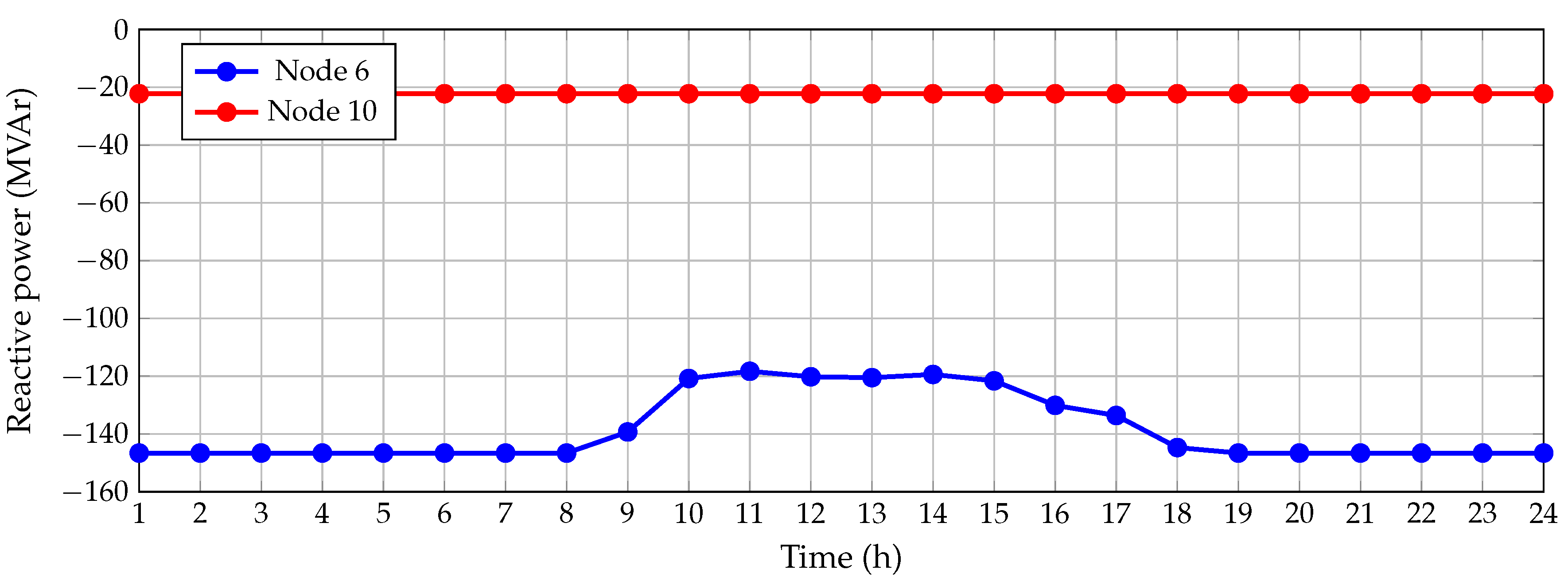On the other hand, when the optimization model (1)–(7) is solved with the BONMIN optimizer in GAMS, the solution obtained corresponds with the installation of two STATCOMs in nodes 6 and 10, with nominal capacities of 146.6292 and 22.2332 MVAr. The total annual operative costs for this solution is MUS $17.3541, which implies a reduction of 30.56%. The total investment cost in STATCOMs for this solution is MUS $1.5748; this implies that the annual costs regarding energy losses were reduced to about MUS $9.2112 per year of operation, which clearly confirms that, with an inversion lower than 2 million dollars per year, more than 9 million dollars worth of energy losses can be recovered.

Figure 6 presents the total reactive power absorbed by the STATCOMs from the power system. Note that this power is absorbed due to the negative symbol, which implies that the STATCOMs remove the excess power capacities from the grid (see model (1)–(7)).

The results, which are presented in Figure 6, show that both STATCOMs work as reactors. The STATCOM located at node 10 absorbs reactive power constantly during all analysis periods, while the STATCOM located at node 6 varies its absorption depending on the grid system load and generator behaviors.

5.2. Multi-Objective Function Optimization

For the multi-objective optimization, we consider that the cost of the energy losses, i.e., $f_1$, is an objective function in conflict with the investments in STATCOMs, i.e., $f_2$. In this sense, we adopt the Pareto front building strategy reported in [29], which is based on the weighting factors associated with the objective functions.

Table 9. Pareto front for the IEEE 24-bus system.

Sol. No.	Nodes (Sizes) (MVAr)	${\mathit{f}}_1$ (MUS $)	${\mathit{f}}_2$ (MUS $)	${\mathit{A}}_{\mathbf{cos}\mathbf{t}}$ (MUS $)
1	$---$	24.9904	0	24.9905
2	$6\left(16.80\right)$	22.9887	0.2060	23.1947
3	$6\left(35.20\right)$	21.1185	0.4120	21.5306
4	$6\left(55.50\right)$	19.4126	0.6180	20.0307
5	$6\left(78.20\right)$	17.9213	0.8240	18.7454
6	$6\left(104.2\right)$	16.9446	1.0301	17.9748
7	$6\left(134.8\right)$	16.2459	1.2361	17.4821
8	$\left\{6\left(149.5\right),10\left(9.60\right)\right\}$	15.9248	1.4421	17.3670
9	$\left\{6\left(144.7\right),10\left(29.80\right)\right\}$	15.7095	1.6481	17.3578
10	$\left\{6\left(141.0\right),10\left(51.60\right)\right\}$	15.5580	1.8542	17.4122
11	$\left\{6\left(136.6\right),10\left(77.00\right)\right\}$	15.4672	2.0602	17.5275
12	$\left\{5\left(5.700\right),6\left(133.8\right),10\left(95.60\right)\right\}$	15.4326	2.2662	17.6989
13	$\left\{5\left(12.50\right),6\left(133.7\right),10\left(112.4\right)\right\}$	15.4236	2.4722	17.8960
14	$\left\{5\left(21.00\right),6\left(139.9\right),10\left(122.0\right)\right\}$	15.4232	2.6756	18.0989
15	$\left\{5\left(33.00\right),6\left(145.3\right),10\left(127.7\right)\right\}$	15.4232	2.8778	18.3011
16	$\left\{5\left(47.50\right),6\left(146.7\right),10\left(134.6\right)\right\}$	15.4232	3.0811	18.5044
17	$\left\{5\left(65.30\right),6\left(147.2\right),10\left(139.5\right)\right\}$	15.4232	3.2843	18.7076
18	$\left\{6\left(147.3\right),8\left(87.70\right),10\left(141.4\right)\right\}$	15.3480	3.4892	18.8373
19	$\left\{6\left(147.6\right),8\left(113.0\right),10\left(143.3\right)\right\}$	15.3480	3.6919	19.0400
20	$\left\{5\left(139.6\right),6\left(148.0\right),10\left(145.4\right)\right\}$	15.4232	3.8788	19.3021

reports all the solutions obtained for the multi-objective approach using the GAMS optimization package and the BONMIN solver. Note that the third and fourth columns demonstrate the multi-objective nature of the optimization problem associated with the optimal installation of STATCOMs in power systems. For example, Solution 1 shows that the solution with no STATCOMs installed has a higher energy loss cost value, i.e., MUS $$24.9904$, while Solution 19 shows the minimum energy loss cost value, i.e., MUS $$15.3480$ with a total inversion of MUS $$3.6919$. However, these solutions are the extremes of the Pareto front and are expected solutions, as between more investments in STATCOMs, more reduction in the cost of the energy losses is expected.

In addition, the results presented in Table 9 allow the following observations: (i) the most attractive nodes for the location of STATCOMs are nodes 6 and 10, respectively; (ii) in Solutions 6–13, the annual operational costs of the grid are lower than MUS $18, which implies that the solution of the linear combination is contained in this range of solutions; and (iii) if the last column in Table 9 is selected as the performance indicator, then Solution 9 corresponds to the minimum annual operative cost with a value of MUS $$17.3578$, which implies a total reduction with respect to Solution 1 (without the location of STATCOMs) of about 30.58%. Note that this solution differs from the linear combination by less than $0.02$%.

Regarding the processing times, the solution of the single-objective optimization problem with the BONMIN solver in the GAMS software takes about 11.26 s, and the multi-objective optimization model with 20 solutions in the Pareto front takes about 242.20 s. These values demonstrate the effectiveness and robustness of the GAMS optimization package for dealing with large-scale MINLP models.

5.3. Application in Distribution Networks

This section presents the validation of the proposed optimization methodology in two radial distribution test feeders composed of 33 and 69 nodes to observe its efficiency when the solution space increases significantly. To calculate the dimension size of the solution space, the following formula can be used [46]:

$$\begin{array}{c}\hfill C_{a,b}=\left(\begin{array}{c}a\\ b\end{array}\right)=\frac{b!}{a!\left(b-a\right)!}\end{array}$$

where a represents the number of shunt devices to be installed and b corresponds to the number of nodes of the network, excluding the slack source. This implies that for the IEEE 33-bus system with three STATCOMs, the dimension of the solution space is $C_{32,3}=4096$, while, for the IEEE 69-bus system, the dimension of the solution space is $C_{68,3}=$ 50,116.

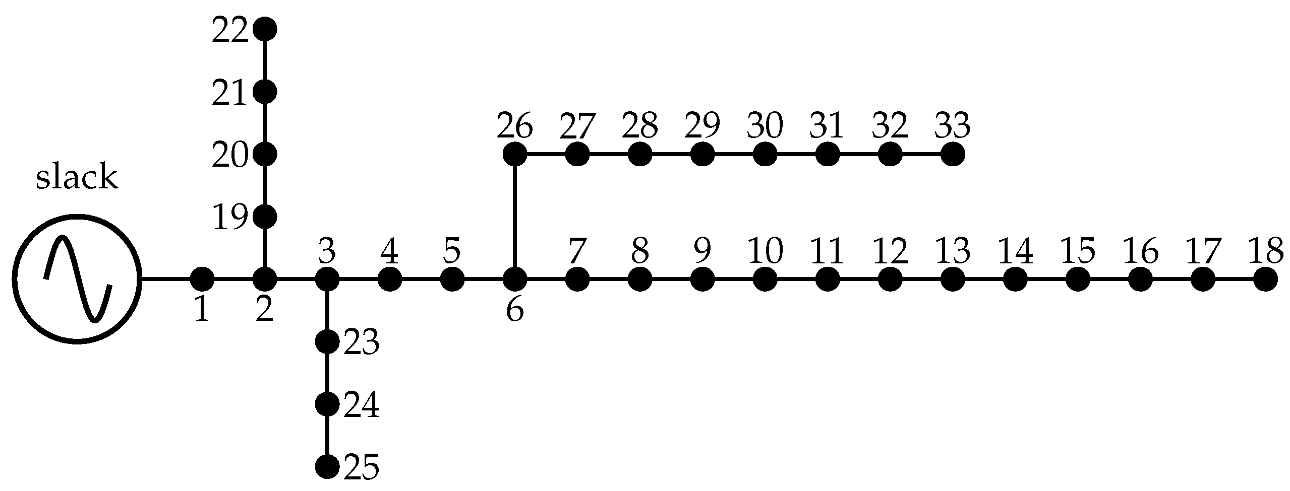
5.4. Numerical Results of the IEEE 33-Bus System

For simulation purposes, in this test feeder, we consider that the loads are combined as follows: 30% for residential and commercial and 40% for the industrial type. The base case for this simulation case corresponds to an annual operative cost of US $142,649.30 when no STATCOMs are installed in the distribution grid; however, when the MINLP model defined in Equations (1)–(7) is solved with the BONMIN solver in the GAMS optimization package, the nodes where the STATCOMs are installed correspond to 14, 30, and 32, with nominal rates of 0.2509, 0.5699, and 0.1656 MVAr, respectively. With these locations of STATCOMs, the annual operating costs are reduced to US $111,499.80, a reduction of 21.84% with respect to the base case. The investment in STATCOMs for this solution is about US $12,551.74, which allows a reduction of about US $43,701.24 regarding the cost of annual energy losses. 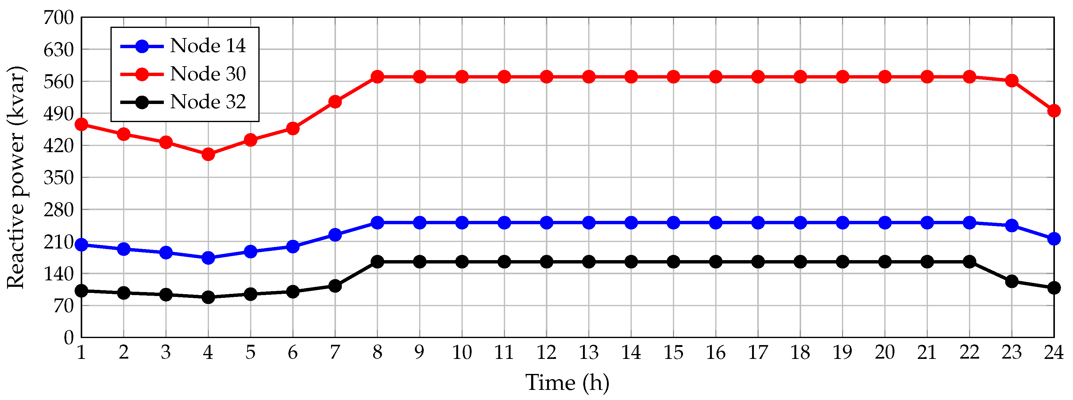This clearly confirms that investments in STATCOMs produce a net profit of US $31,149.50 per year of operation. Finally, Figure 7 presents the reactive power injections (capacitive compensation) of the STATCOMs in nodes 14, 30, and 32, respectively.

From the results presented in Figure 7, it is possible to observe the following: (i) during periods 1–8, all the STATCOMs work with capacitive power injections less than their nominal rates, which is caused by the demand behaviors that in this time period have low values (see Table 7); (ii) during periods 8–22, the STATCOMs work with their nominal capacities, which is an expected behavior, as in these time periods, the loads are higher than 70% of the peak load condition; (iii) for the periods of time higher than 22 h, the amount of reactive power injected by the STATCOMs starts to decrease (with regards to the nominal capability), as the loads in these periods are lower than 60% of the peak load condition; and (iv) the total processing time of the GAMS software for solving this problem is about 23 s, which is a short time to solve a complex MINLP model with more than 1500 variables.

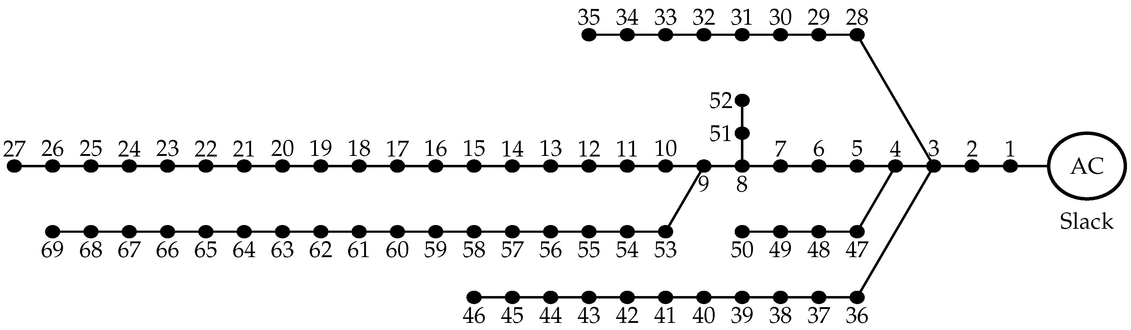
5.5. Numerical Results in the IEEE 69-Bus System

For this test feeder, the same combination of loads of the IEEE 33-bus system are considered, which implies that, for the benchmark case (i.e., without STATCOMs installed), the annual operative costs of the grid is 151,705.9839 USD/year. Once the optimization methodology is used to determine the optimal site and size of the STATCOMs in the IEEE 69-bus system, the annual operative cost of the network is reduced to 115,714.0404 USD/year, which corresponds to annual energy loss costs of 102,241.5784 USD/year and an inversion in STATCOMs of 13,472.4620 USD/year. These results imply that the reduction of the annual operative costs of the network after installing the STATCOMs is about $23.72\%$. The nodes where the STATCOMs are located correspond to 11 and 61, with nominal rates of $0.1579$ and $0.9017$ MVAr, respectively.

6. Conclusions and Future Works

The problem of the optimal siting and sizing of STATCOMs in electrical power systems with radial and mesh structures was addressed in this research from the exact mathematical optimization point of view with the help of the BONMIN solver in the GAMS optimization environment. Numerical results for the IEEE 24-, IEEE 33-, and IEEE 69-bus test systems demonstrate a reduction in the annual operating cost of $30.56$%, $21.84$%, and $23.72\%$, respectively, when the STATCOMs are optimally sized and located.

In the IEEE 24-bus system, the multi-objective nature of the problem of the optimal placement and sizing of STATCOMs in power systems was verified, as the cost of annual energy loss is an objective function in conflict with the investment costs in STATCOMs. This Pareto front conformed with the multi-objective optimization approach using weighting factors, where the difference between both extreme solutions are MUS $9.5 regarding the cost of energy losses and MUS $3.8 regarding the inversions in STATCOMs. The single-objective function optimization model and the minimum annual operating costs reported by the multi-objective optimization model (see Solution 9 in Table 9) are practically the same solution, as the difference between these was $0.02$%. In both cases, the nodes 6 and 10 were identified as the most promising nodes for installing STATCOM devices with capacities of about 140 and 30 MVAr, respectively.

The processing time of the single-objective model in the IEEE 24-bus system was about 11 s, while the multi-objective model was solved in approximately 242 s. In the case of the single-objective model for the IEEE 33-bus system, this processing time was about 23 s, whereas, for the IEEE 69-bus system, this processing time was about 71 s. These results confirm the effectiveness and robustness of the GAMS optimization package and the BONMIN solver in solving the MINLP models with more than 1000 variables between the integer and continuous ones in a few seconds.

In the future, the following studies can be conducted: (i) the development of a mixed-integer convex reformulation of the studied problem to ensure the global optimum finding via conic and/or semidefinite programming; (ii) the development of a hybrid master–slave optimization algorithm based on metaheuristics and power flow to solve the optimization problem sequentially; and (iii) the extension of the studied problem to three-phase unbalanced networks.