Article

A Mobile Robot Position Adjustment as a Fusion of Vision System and Wheels Odometry in Autonomous Track Driving †

by
Jarosław Zwierzchowski
1,*,
Dawid Pietrala
2,
Jan Napieralski
1 and
Andrzej Napieralski
1
1
Department of Microelectronics and Computer Science—DMCS, Lodz University of Technology, 90-924 Lodz, Poland
2
Department of Automation and Robotics, Kielce University of Technology, 25-314 Kielce, Poland
*
Author to whom correspondence should be addressed.
This paper is an extended version of our paper published in the 27th International Conference “Mixed Design of Integrated Circuits and Systems”, Lodz, Poland, 25–27 June 2020.
Appl. Sci. 2021, 11(10), 4496; https://doi.org/10.3390/app11104496
Submission received: 19 April 2021 / Revised: 9 May 2021 / Accepted: 10 May 2021 / Published: 14 May 2021

Abstract

:
Autonomous mobile vehicles need advanced systems to determine their exact position in a certain coordinate system. For this purpose, the GPS and the vision system are the most often used. These systems have some disadvantages, for example, the GPS signal is unavailable in rooms and may be inaccurate, while the vision system is strongly dependent on the intensity of the recorded light. This paper assumes that the primary system for determining the position of the vehicle is wheel odometry joined with an IMU (Internal Measurement Unit) sensor, which task is to calculate all changes in the robot orientations, such as yaw rate. However, using only the results coming from the wheels system provides additive measurement error, which is most often the result of the wheels slippage and the IMU sensor drift. In the presented work, this error is reduced by using a vision system that constantly measures vehicle distances to markers located in its space. Additionally, the paper describes the fusion of signals from the vision system and the wheels odometry. Studies related to the positioning accuracy of the vehicle with both the vision system turned on and off are presented. The laboratory averaged positioning accuracy result was reduced from 0.32 m to 0.13 m, with ensuring that the vehicle wheels did not experience slippage. The paper also describes the performance of the system during a real track driven, where the assumption was not to use the GPS geolocation system. In this case, the vision system assisted in the vehicle positioning and an accuracy of 0.2 m was achieved at the control points.

1. Introduction

The article describes the implementation of algorithms to determine the position and orientation of the mobile robot in a certain coordinate system without the participation of the GPS positioning system. Authors divided the described task into two subsystems constantly sending messages to each other via the UART bus. The first subsystem consists of programs located in the robot control system and determines the robot’s trajectory calculated from the vehicle wheels. This is called wheels odometry and it is widely used in the automotive industry. A general discussion of this solution is described in [1,2]. Currently, designers of modern solutions to increase the accuracy of the determined robot position, use a combination of many independent positioning systems. Therefore, the authors added to the wheels odometry a vision system. A vision system with an implemented SLAM (Simultaneous Localization and Mapping) algorithm is the most often described in the literature [3]. Visual odometry is a technique used by many different robots. Ichimura uses 3D-Odometry in the bike robots [4]. Tanaka et al. deploy odometry in the robot which specializes in the exploration and sampling of the seafloor [5]. Current research indicates that wheels odometry are crucial for robot self-localization [6]. Such an approach may be implemented using not only the camera but also IMU and wheel encoder [7]. Jung et al. proposed a solution based on MEMS IMU efficient in urban areas [8]. Chaudhari et al. proved that Cartesian odometry and PID algorithm may significantly increase the accuracy of path planning [9]. Zhang et al. present odomerty method to estimate the pose of the robot using ORB features extraction [10]. To increase the accuracy of the self-localization process. Lin et al. proposed a method based on ceiling vision [11]. Current approaches use deep learning techniques to improve visual odometry [12]. Aladem et al. proposed a solution which enables application of visual odometry in non-cooperative environment, for example in the night [13]. The partial differential of the pixel grayscale is another method for improving the performance of visual odometry in difficult conditions [14]. In this article, the vision system only provided position corrections, and was geared toward finding characteristic landmarks. The problem with landmarks was studied by [15]. The OpenCV library algorithms are used [16], where the authors use ARTags in augmented reality. Due to the autonomous movement of the robot, the issue of safety arises during the physical interaction of a human with a robot [17].
The vehicle presented in this paper belongs to a group of vehicles called unmanned ground vehicles (UGV), where an important task of their creators is to develop navigation algorithms to improve their ability to operate in difficult terrain [18]. The UGVs are robots that move and make decisions based on various algorithms both deterministic and artificial intelligence. While driving, vehicles use their sensors to avoid obstacles or locate their position in the environment. These abilities make that, this kind of vehicles are increasingly important in terms of replacing humans in many missions that are dangerous for them. The vision system described by the authors aims to remove positioning errors coming from other sensors of the robot. This error is often the cause of slippage. There are studies that reduce slippage not only for wheeled vehicles [19].
To check the correctness of the implemented subsystems, a mobile robot was designed and built [20]. In addition, many tests were performed on the test track. This track was precisely measured and a map was made based on these measurements. Control points and the position of graphic markers—ARTags—were placed on the map. The experiment assumed that the robot autonomously would be able to move from the starting point to the next and subsequent checkpoints with the greatest accuracy. Besides, if the robot calculated that a checkpoint was reached, the blue lamp mounted on its board stated to flash.
By design, numbers from 0 to 16 are encoded in the ARTags. To accurately determine the position of the robot, the vision system needed to recognize three markers. If two markers had been detected, two robot positions were determined and fortunately, one of which could easily be rejected. If one marker was detected, the robot could be located with lower accuracy, one was positioned on the circle indicated by the distance between the robot and the marker. To calculate the distance to the markers, a specially designed head with two cameras was used. The appearance of the head and the ARTag are shown in Figure 1.
The software that interpreted the robot’s space was initially tested on a laptop with an Intel Core i7 processor and 32 GB RAM, which at 1024 × 760 resolution allowed to run the ARTag recognition algorithm 15 frames per second. The vision system communicated with the robot’s main processor via a serial bus and transmitted the numbers of founded markers and the distances to them. Information from the wheel odometry was also transmitted to the main processor. Ultimately, the important step of the whole task was to combine the subsystems described above into one decision-making control system, i.e., calculating signals fusion. Tests for the accuracy and speed of the vision system were described in [21]. A general structure of the robot system is shown in the Figure 2.
All algorithms pertaining to the wheels odometry were implemented in C language and are flashed in the STM processor. The vision system was written in C++ language.
A photograph of the robot is shown in Figure 3.

2. Determining Vehicle Position

In this section, the description of the method for acquiring information about the position and orientation of the mobile robot, both from sensors determining travelled distance and the vision system, will be presented. At the end of the section, the method for fusing those signals will be described.

2.1. Position from Wheels and IMU

The current relative position of the mobile robot in two-dimensional real space was determined by a vector of two coordinates p w = [ x , y ] . Those coordinates were determined according to Equation (1)
x = sin θ v x d t + x 0 , y = cos θ v y d t + y 0 ,
where: θ —current vehicle yaw angle relative to the axis Y, v x , v y —vehicle speed, x 0 , y 0 —initial vehicle position. In order to determine the current relative position of the mobile robot, information about the current speed and angle relative to the Y-axis (azimuth) in some coordinate system is necessary. For this purpose, each of the robot wheels is equipped with a DC motor with an incremental encoder and also for each wheel there a PID controller algorithm was implemented to control the velocity. The control system, at each calculation step, maps the current linear vehicle speed from known angular velocities of individual wheels and geometrical dimensions. At the same time, azimuth is read from an inertial navigation system equipped with an accelerometer, gyroscope and magnetometer.

2.2. Position from ARTags

Let’s define image I as a two-dimensional array containing grayscale intensity of the recorded pixel, I : Ω R 2 R + ; ( x , y ) I ( x , y ) , where Ω is the domain of the image. Point P = ( x , y , z ) T from 3D space is donated as p = ( x , y ) T Ω . The vision system has been developed and will be presented in the 6 steps described below.

2.2.1. Edge Detection—Canny Algorithm

First, all edges of the image should be detected. The edge is an ordered significant change in the adjacent pixel values. This means that if I ( x k , y 1 ) > I ( x k , y 2 ) , a vertical edge is obtained. In the simplest case, the edge is gained (discovered) using the equation
I ( x , y ) x I ( x + 1 , y ) I ( x , y ) 1 .
However, we can correctly obtain the edge only if the image is passed throught a low-pass filter, for example, a Gaussian filter h ( τ , σ ) , because the edge will hide in the noise. This means that the final form of the edge detection filter will be equal to
I = ( h ( τ , σ ) × I ( x , y ) ) x , ( h ( τ , σ ) × I ( x , y ) ) y ,
where in Canny edge detector threshold τ > 0 and standard deviation σ > 0 . Next step is as follows. If I T I is larger than the predefined gradient threshold and is in local maximum along the gradient, set this pixel as the edge. The final step of the algorithm is to differentiate the one-point edge from the hysteresis of two thresholds [22].

2.2.2. Contour Detection and Polygonal Approximation

Next, the contours of the object are needed, whose edges were obtained in the previous step. For this purpose, the algorithm of the polygon contour description is proposed. Its main goal is to specify the vertices of the polygon according to the Ramer–Douglas–Peucker algorithm. Let’s define vector D = [ p 0 p 1 p n ] describing the points lying on the contour of the object. Define the segment L k with the beginning at point p 0 and ending at point p n . Additionally, determine all lines perpendicular to this segment L k passing through the points from vector D and determine the longest norm L 2 d k for this straight line
{ p D : m a x p i L k 2 = d k } .
If d k > T , set a new segment L k + 1 at the beginning at current L k segment beginning and end at point p k , for whose d k has been determined. In Equation (4) T is arbitrarily selected threshold. Save point p k as the vertex of the polygon in vector D ^ . If d k < T calculate L k + 1 such that the beginning is at point p k , and the end at point p n . Reassign d k + 1 according to Equation (4). Finish the algorithm if the L segment cannot be created.

2.2.3. Rejecting Incorrect Markers

The next step of the graphic markers recognition task is to choose appropriate candidates based on the following criteria. The first criterion is to check whether vector D i ^ defining vertices has 4 elements. Next, it is important to check also, whether the vertices form closed contours, i.e., whether they depict geometrical figure. The last two tests check if the geometric figure is convex and whether the distance between consecutive segments resulting from the fusion of points in vector D ^ is big enough. Vector D i ^ , which fulfills these tests is saved as a candidate containing the marker shape.

2.2.4. Removing Perspective and Warping Algorithms

The candidate selected in the previous step may include a marker wiht a number. We need to find position of a camera coordinate system to make vector D i ^ containing vertices of any quadrangle to be able to convert into vertices of the square. In this work, the warping perspective method with homography A was used. Next, knowing the transformation matrix the equation could be used I ^ ( x , y ) = A × I ( x , y ) to distort the image.

2.2.5. Detecting Marker Frame and Reading Its Code

Having determined picture from the previous step, it is possible to start reading the tag code. To do this, the image is divided into a grid of 9 × 9 squares, then a count of the white pixels in each square is performed. If their number is higher than the defined threshold, then the square represents the binary number 1, oppositely the square is assigned to value 0. The resulting matrix containing binary numbers is compared with the code patterns. Each marker has a frame with two squares thickness.

2.2.6. Calculation of the Position and Orientation of the Marker

The proposed equation for a calibrated camera can be written as follows
λ [ u , v , 1 ] = K [ R | t ] [ X , Y , Z , 1 ] T ,
where K is the matrix of the internal camera parameters containing the focal length and the physical centre of the image, matrix [ R | t ] is the matrix of the external camera parameters containing rotations and translations of the camera coordinate system relative to global coordinate system. The task is to calculate matrix Q from the linear equation Q × H = 0 , where H = K [ R | t ] . Using the homogeneity of the image points p i the equations could be written as, P i T h 1 T + 0 × h 2 T u i P i T h 3 T = 0 and 0 × h 1 T + P i T h 2 T v i P i T h 3 T = 0 , where h i , i = 1 , 2 , 3 are rows of the unknown matrix H. To obtain the matrix H, the Singular Value Decomposition (SVD) method shall be used. At least four p points on the image I and their equivalents in 3D are needed to solve the equation. As a result of calculating SVD one of the matrices is the matrix [ R | t ] , where t = [ x , y , z ] , from which we will determine the distance between the vehicle and the marker d v = λ x 2 + y 2 + z 2 .

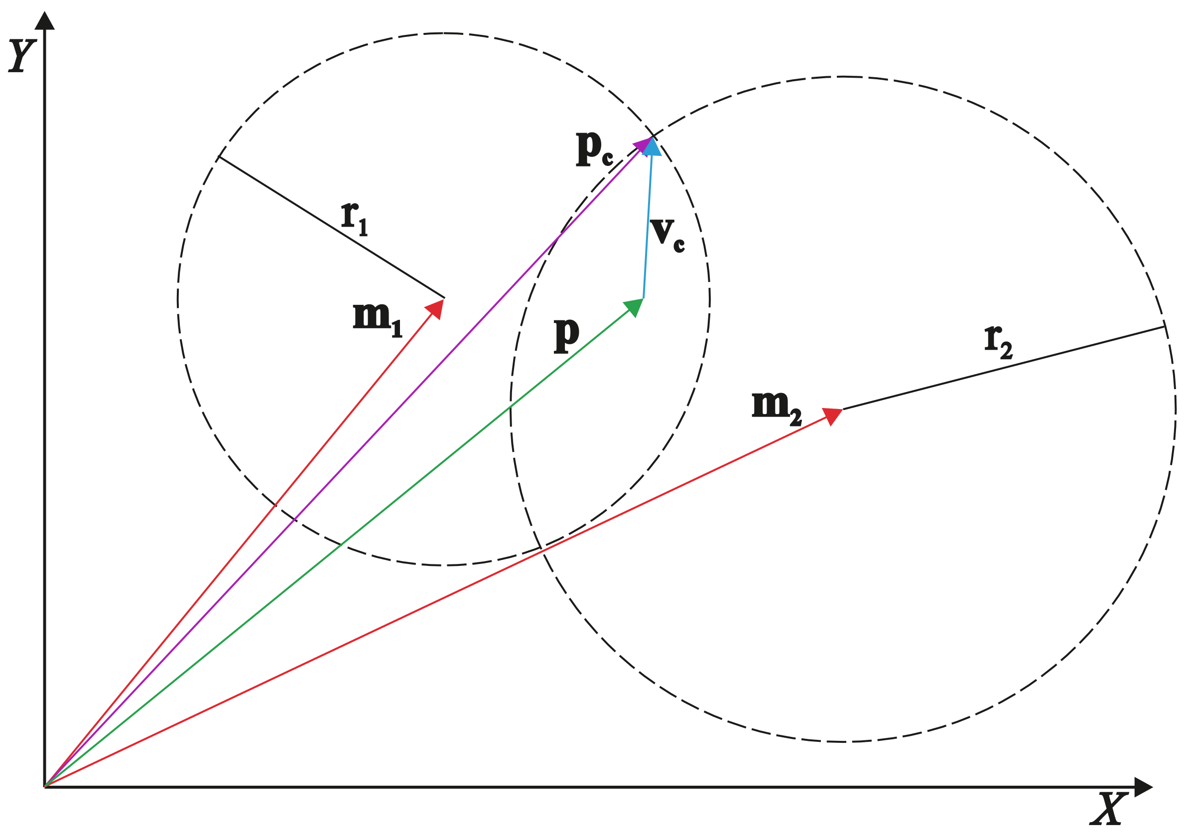
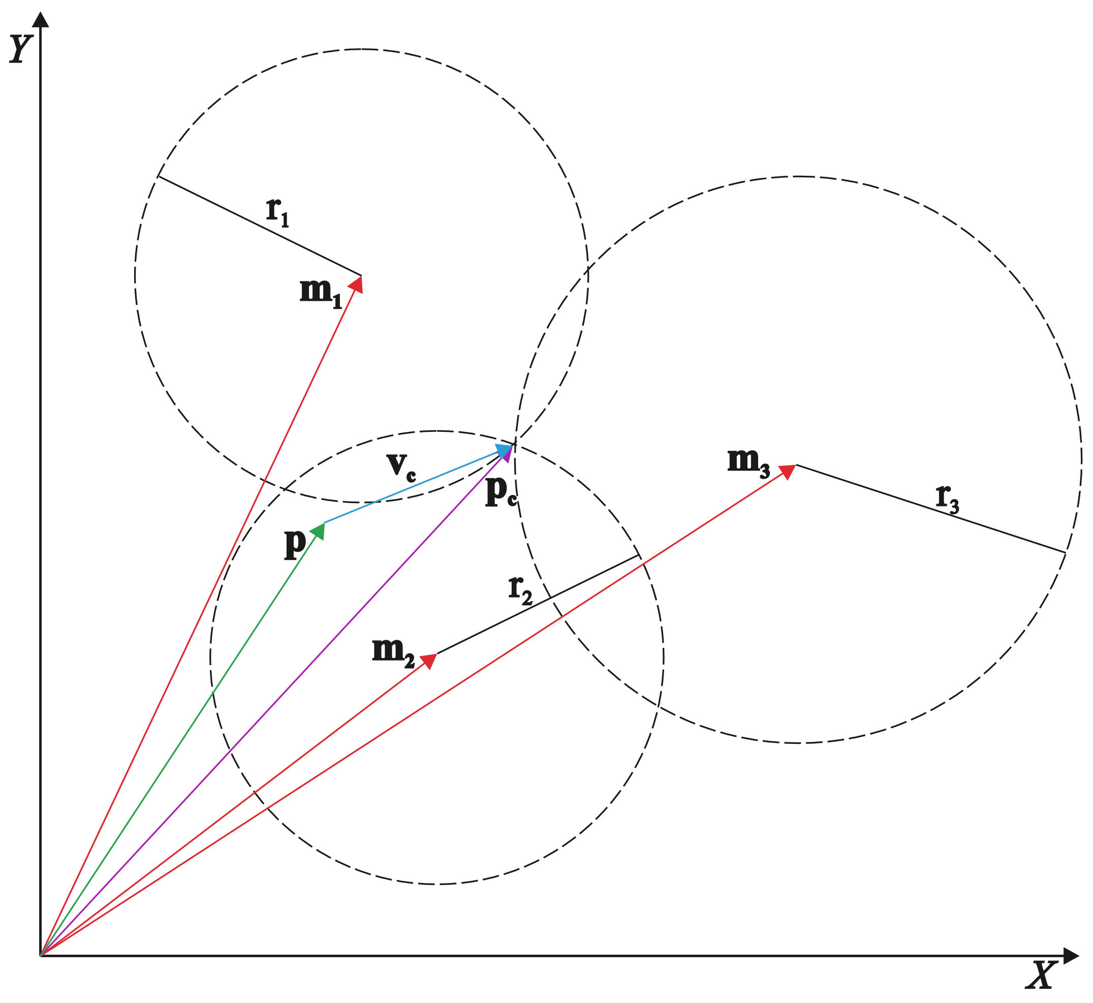
2.3. Fusion of Wheels and Vision Signals

This method of determining the position of a robot is exposed to errors, for example from the wheel slip. Additionally, the error of the currently determined position is the sum of all errors that have occurred since the beginning of the journey. To determine the relative position with correction determined according to the method presented above, a comparison of results from the vision system was used. A set of markers were placed into a workspace of the mobile robot, whose values and positions were known. The vision system sent information about numbers of currently detected markers and distance to them, to the robot controller. Then, based on the information received, correction was determined according to the following procedure. There were three cases.
The first occurs when the vision system correctly recognizes one marker. This is shown schematically in Figure 4, where: m —vector determining the position of the marker, p —vector of the robot position determined from the odometry system, p c —vector determining the corrected position of the robot, v c —correction vector, r—distance from the marker obtained from the vision system. The corrected vehicle position is calculated as a point on a circle with a radius equal to the distance to the marker obtained from the vision system and the center point of the marker that is closest to the current vehicle position determined from the odometry system.
The second case takes into account the situation when the vision system correctly detects two markers simultaneously (or the subsequent markers appear with a time interval smaller than 0.3 s). This is schematically illustrated in Figure 5, where: m i —vector defining the position of the marker i, p —vector of the robot position determined from the odometry system, p c —vector defining corrected robot position, v c —correction vector, r i —distance from the marker i obtained from the vision system. In this situation, the corrected robot position is in one of two places, which are the intersection of two circles with radii equal to vehicle distance from the markers and the centres lying in the markers point. The robot algorithm chooses the solution, which is closer to the robot’s currently determined odometry position.
The third case takes into account the situation when the vision system correctly detects three or more markers simultaneously (or the subsequent markers appear with a time interval smaller than 0.3 s). This is schematically illustrated in Figure 6, where the designations were adopted as in Figure 5. In this situation, three markers are selected. The corrected robot position is determined as the intersection of all three circles, with radii equal to the distance from the markers and with centres at the marker points.
In the first case, that is, when only one marker is detected, the vehicle is located on a circle with a radius that is the distance of the vehicle to the marker. In this case, its position can be estimated. The vehicle is located on the arc of the circle closest to the position calculated from the wheels odometry. In the second case, after detecting two markers, the vehicle can be located in two positions, which are the intersections of circles determined by the distances to these markers. The closest intersection to the current vehicle position is selected. In the third case, the vehicle position is determined uniquely and the vehicle is located at the intersection of three circles. Corrected data is immediately sent to the robot control system and the tentative robot position is updated, but with provision, that the position taken from the vision system always has higher priority.

3. System Tests

In this section, the results which contain accuracy tests obtained in the laboratory and real test during international competition, which took place in Poland, are presented.

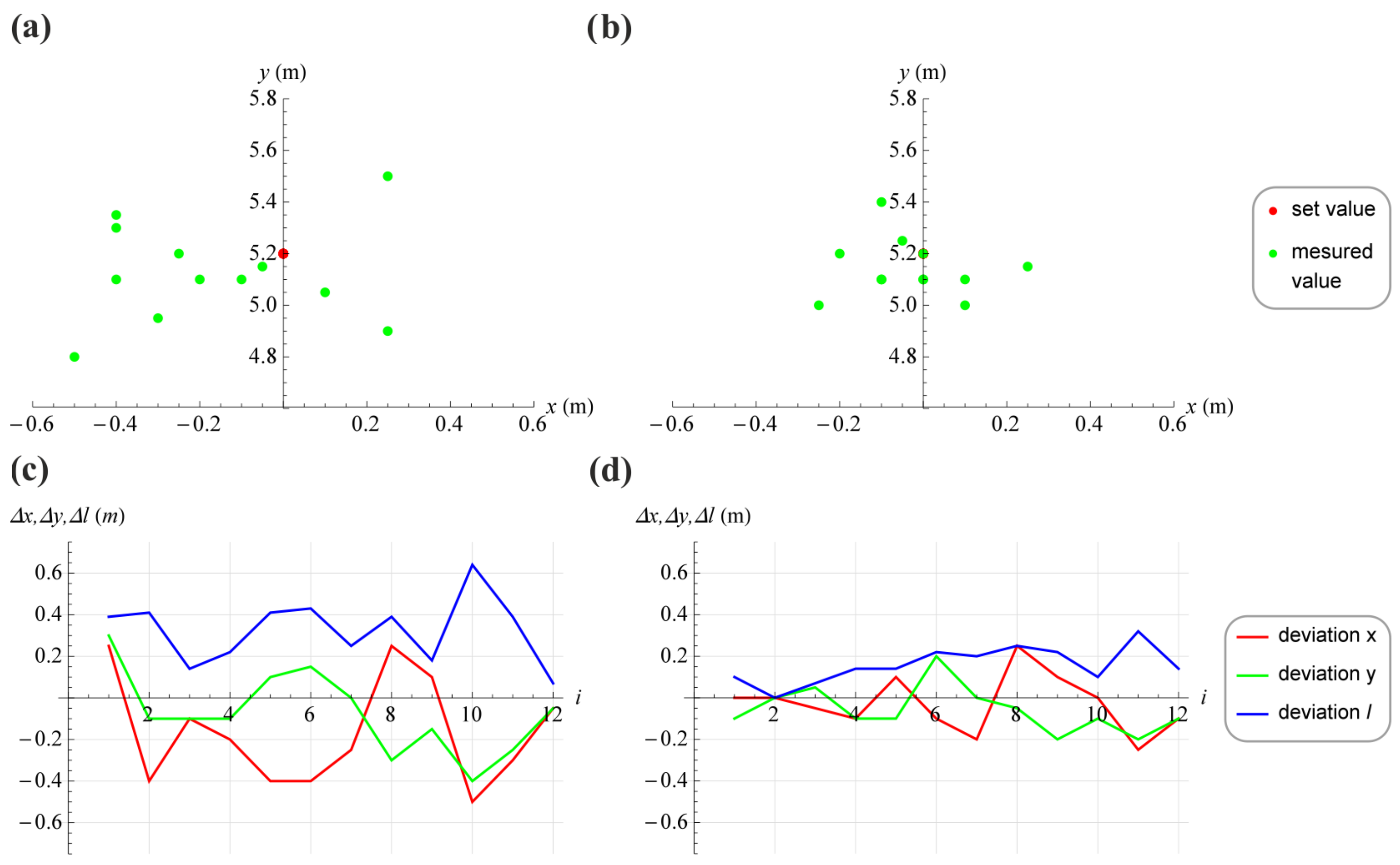
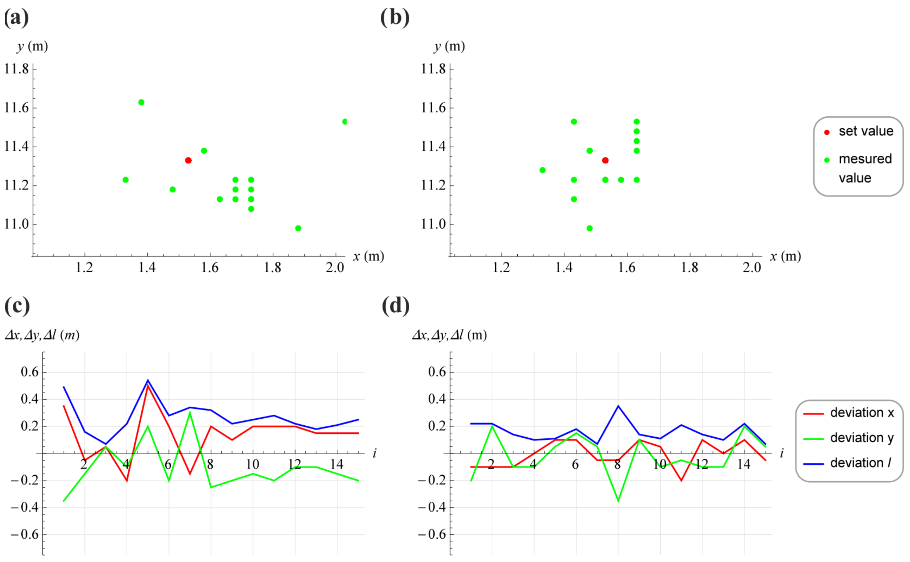
3.1. Test in the Laboratory

The first stage relates to testing the position accuracy from the vehicle to the desired position on the map. Figure 7 shows a vehicle equipped with a vision system and few ARTags located on the test track in the laboratory.
Tests on the correctness of estimating the closest distance to the indicated target were carried out in good lighting conditions, thanks to which the differences between the actual distance and the one determined by the algorithm were small, with the average distance of up to 3 m, the relative errors were in most cases smaller than 1% as shown in Figure 8.
For worse conditions, for example underexposure, the maximum detection distance was significantly reduced. The strong light falling on the marker could even prevent detection. A detailed description was presented in [21] where it was noted that absolute measurement errors increase with the distance. The most accurate measurements were obtained for distances up to 3 m and this corresponds to the distance for which the camera was calibrated. In the test conducted in the laboratory, there were five marker destinations that the robot had to travel to.
In every test, the robot made 76 drives on a randomly selected point and stopped there. Exactly 12 ARTags were placed on the test track. Each ARTag was 180 mm × 180 mm in size. During one test, the robot covered about 668 m. The first test was an autonomous drive with the vision system turned off. This means that only wheel odometry was taken into account with some undesirable drift coming from the inertial sensor. We can see driving accuracy results marked by the letter (a) in Figure 8, Figure 9, Figure 10, Figure 11 and Figure 12. In the figures we marked by the letter (c), the position deviations in the axis x and y with cameras turned off. The exact same sequence was reproduced in the second experiment with the vision system and odometry turned on (every letter (b) in the figures). Deviations in this case are presented in figures (d). The system had two cameras on board.
Figure 13 presents differences between set and reached positions in the 76 driving experiments. Figure 13a is a graph representing position accuracy in the x direction with cameras turned off and Figure 13c with cameras on. Comparing Figure 13b,d, which represent the position deviations, we can see that the case with cameras on the rover increased its position accuracy. Figure 13e,g represent the position accuracy in the y direction. When cameras were turned on, the accuracy was better, this is shown in Figure 13f,h. Figure 13i,j show, respectively, the distance deviation when the cameras are turned off and on. Those two show that there was a significant improvement in the accuracy in determining the rover position when we applied vision system distance calculation to the wheel odometry. Table 1 shows the result of quantifying the positioning accuracy without cameras and with them. The sum of the deviation modules, measured in the individual axes and the sum of the distance deviations were used as the indicator. It should be noted that the vison system increased vehicle position accuracy by about 50 percent.

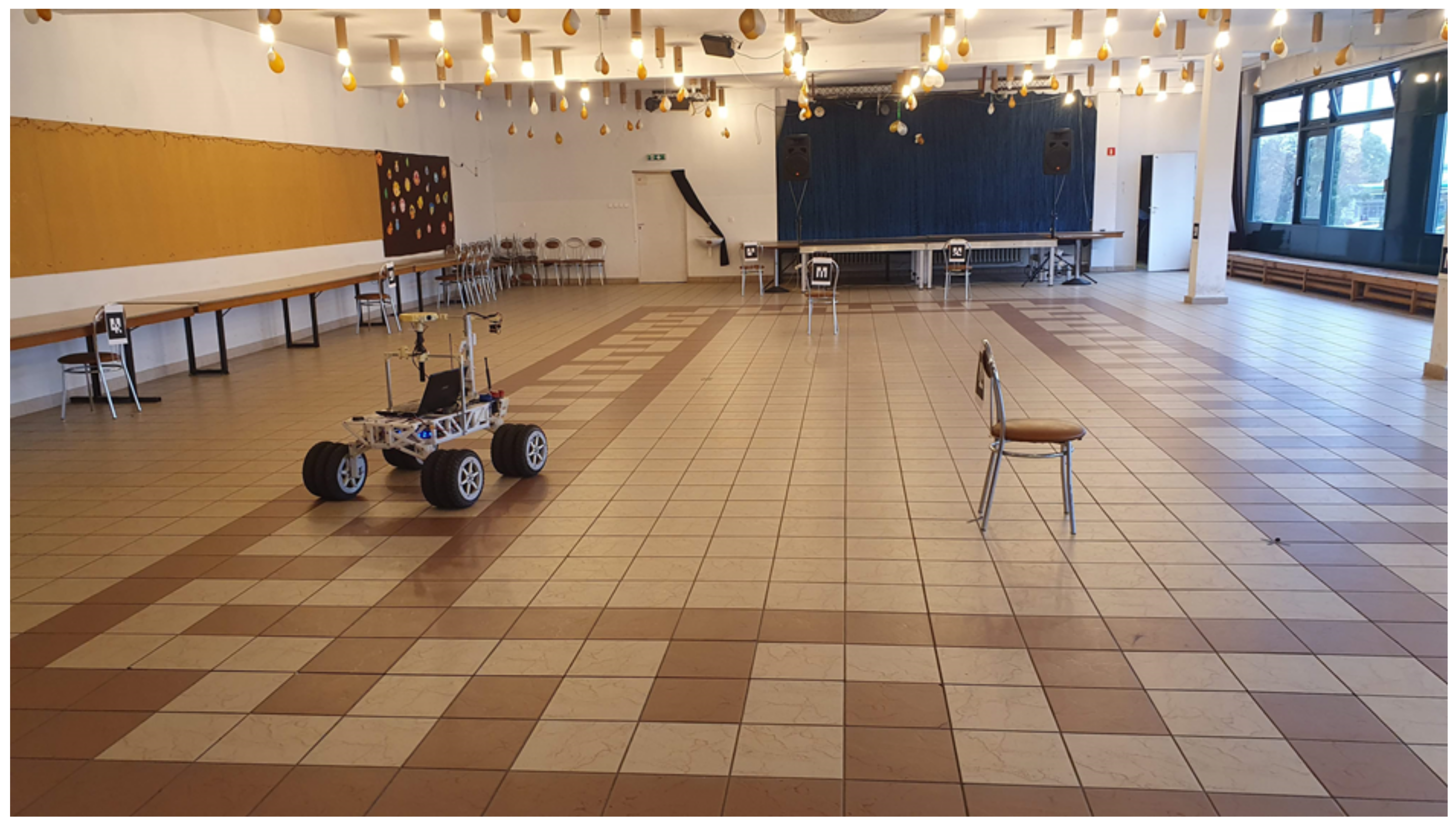
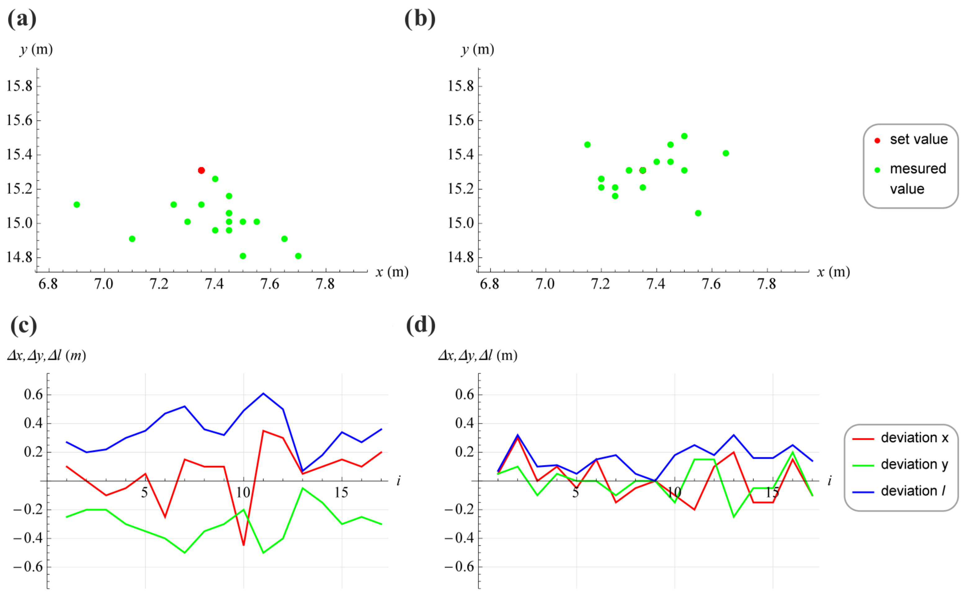
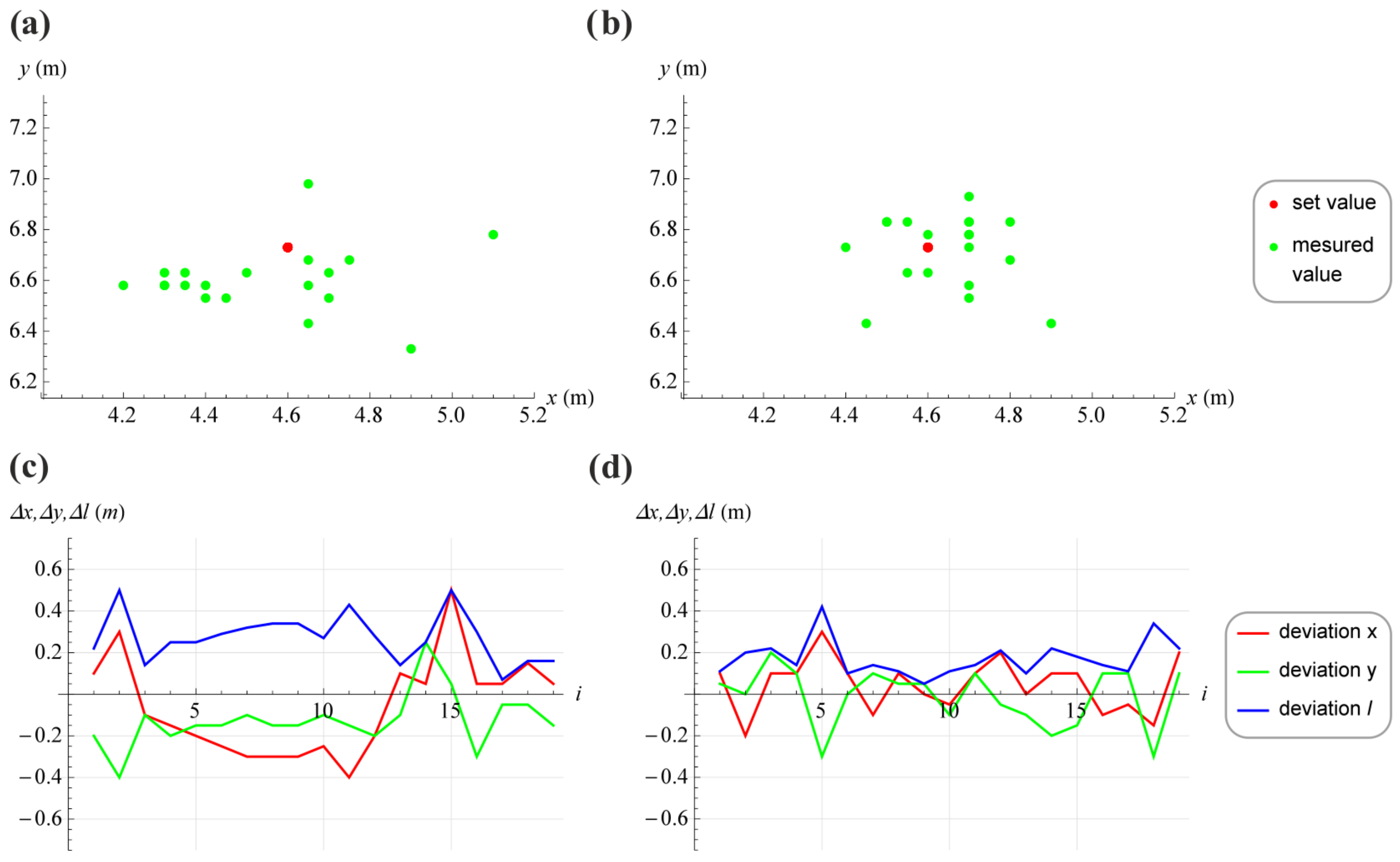
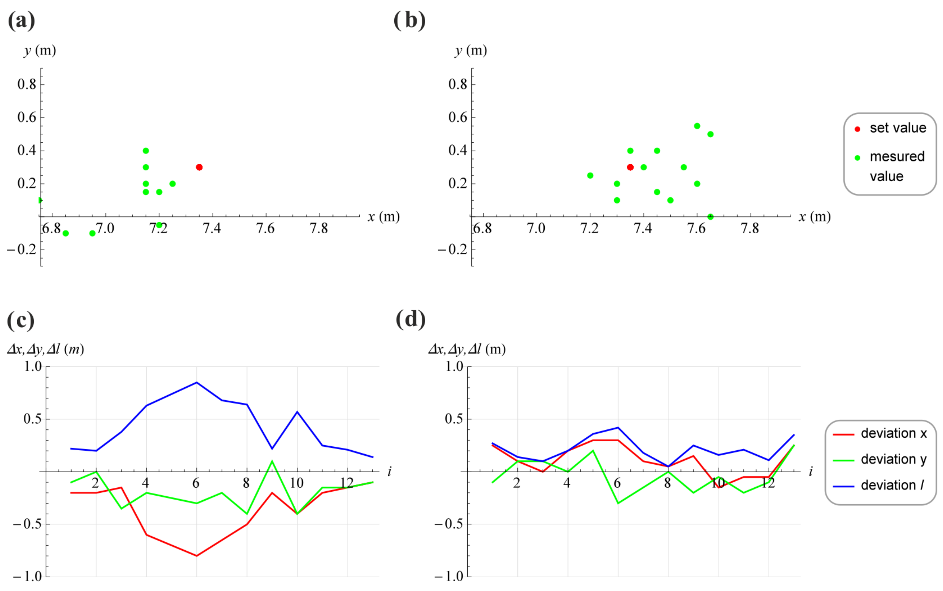
3.2. Test in the Real Environment

The second stage of the test was performed in Kielce University of Technology and at the European Rover Challenge international competitions in 2018 and 2019. Figure 14 presents a map of test track with control points (letter W), graphic markers (letter L) where the point number was coded using ARTags.
The places with obstacles were marked in black (letter R). The robot’s position on the track was marked on the map with a red dotted line. The side of the map grid shows a resolution of 1m. In Figure 15, the arrows show the corrections made during the driving. The black arrow indicates the correction made after detecting the markers number L4 and L5, while the red arrows indicate where the control system made corrections after detecting the L6 and L7 markers. As mentioned in [21], the recognition range of the system was limited to about 6 m, therefore corrections are calculated near the markers. During the main drive at the competition, the vehicle reached the checkpoints with the following accuracy. Checkpoints W1—2 cm, W2—5 cm, W3—20 cm. The W4 checkpoint was very difficult to reach due to the large wheels slip of the vehicle and the fact that the vision system did not have two markers in its field of view. The vehicle control system did not make position correction and decided that the vehicle had reached the checkpoint without disruption. The same situation happened with the WX point, which was hidden behind the hill.

4. Conclusions

The paper describes the automatic driving system of a mobile vehicle, which was equipped with two independent systems based on which the vehicle’s position on the test track can be determined. The experiment assumes that GPS cannot be used. The first of the implemented systems calculated the robot positions from the robot wheels. This is the main system of the robot positioning in space, but its main disadvantage is the fact that the larger the distance travelled by the robot, the more positioning error increases. Therefore, the authors decided to develop a system that provides corrections from an independent system that gives an absolute measurement to known characteristic points with a well-known location on the track. The measurement to the markers was carried out using a vision system and if the marker or markers appeared in the field of view of the camera, the system began to use the detection algorithm and determines the correction needed. Additionally, the vehicle algorithm informed about this fact by lighting the blue lamp on board. The places where the system made corrections are shown in the screenshots and marked with arrows. During real track tests, the vehicle performed 15 drives. The robot was placed on the starting line and then we measured the positioning accuracy. It should be noted that the vehicle was not able to complete the full test drive, when the vision system was turned off, despite being equipped with a simple wheel slip detection system. This result was expected, due to the very sandy ground. A more sophisticated system would need to be used in the future. When the vision system was turned on, an approach to the first checkpoint was obtained with an accuracy of 2 cm, the worst result was obtained at the last checkpoint and it was 20 cm. This was because the checkpoint was laying at the top of a very steep hill. In this case, it may help, the algorithm described in [19]. It can be concluded that the laboratory tests overlapped with the real track tests. The addition of the vision system made the autonomous task possible to complete across the entire test track, with the required accuracy of 50 cm. Especially, when the obtained results were compared with GNSS with RTK results ±15 cm presented in [23].
During further research, it is worth considering replacing known graphical markers such as ARTags with arbitrary feature points from the vehicle environment. This will allow authors to determine the position with higher accuracy. Currently, due to the increasing computational efficiency of microprocessor chips, the authors plan to implement vehicle tracking using robust SLAM and sparse point cloud on the vehicle board.

Author Contributions

Supervising A.N.; conceptualization J.Z. and D.P.; methodology, J.Z.; software, J.Z. and D.P.; validation, J.N., J.Z. and D.P.; formal analysis, J.Z., J.N.; investigation, J.Z.; data curation, D.P.; writing—original draft preparation, J.Z.; visualization, D.P. All authors have read and agreed to the published version of the manuscript.

Funding

This research was funded by Lodz University of Technology, 116 Zeromskiego Street, Lodz 90-924, Poland and Kielce University of Technology, 7 1000-lecia P.P. Avenue, Kielce 25-314, Poland.

Institutional Review Board Statement

Not applicable.

Informed Consent Statement

Not applicable.

Data Availability Statement

Not applicable.

Acknowledgments

Authors would like to thank the Kielce University of Technology IMPULS Team, who won European Rover Challenge 2018, 2019 in Poland and University Rover Challenge 2019 in Utah USA.

Conflicts of Interest

The authors declare no conflict of interest.

References

  1. Scaramuzza, D.; Fraundorfer, F. Visual Odometry Part I: The First 30 Years and Fundamentals. IEEE Robot. Autom. Mag. 2011, 18, 80–92. [Google Scholar] [CrossRef]
  2. Scaramuzza, D.; Fraundorfer, F. Visual Odometry: Part II: Matching, Robustness, Optimization, and Applications. IEEE Robot. Autom. Mag. 2012, 19, 78–90. [Google Scholar] [CrossRef] [Green Version]
  3. Cadena, C.; Carlone, L.; Carrillo, H.; Latif, Y.; Scaramuzza, D.; Neira, J.; Reid, I.; Leonard, J.J. Past, present, and future of simultaneous localization and mapping: Toward the robust-perception age. IEEE Trans. Robot. 2016, 32, 1309–1332. [Google Scholar] [CrossRef] [Green Version]
  4. Ichimura, T. 3D-odometry using tactile wheels and gyros: Localization simulation of a bike robot. In Proceedings of the 2016 16th International Conference on Control, Automation and Systems (ICCAS), Gyeongju, Korea, 16–19 October 2016; pp. 1349–1355. [Google Scholar] [CrossRef]
  5. Tanaka, Y.; Semmyo, A.; Nishida, Y.; Yasukawa, S.; Ahn, J.; Ishii, K. Evaluation of underwater vehicle’s self-localization based on visual odometry or sensor odometry. In Proceedings of the 2019 14th Conference on Industrial and Information Systems (ICIIS), Kandy, Sri Lanka, 18–20 December 2019; pp. 384–389. [Google Scholar] [CrossRef]
  6. Brossard, M.; Bonnabel, S. Learning wheel odometry and IMU errors for localization. In Proceedings of the 2019 International Conference on Robotics and Automation (ICRA), Montreal, QC, Canada, 20–24 May 2019; pp. 291–297. [Google Scholar] [CrossRef] [Green Version]
  7. Liu, J.; Gao, W.; Hu, Z. Visual-inertial odometry tightly coupled with wheel encoder adopting robust initialization and online extrinsic calibration. In Proceedings of the 2019 IEEE/RSJ International Conference on Intelligent Robots and Systems (IROS), Macau, China, 3–8 November 2019; pp. 5391–5397. [Google Scholar] [CrossRef]
  8. Jung, J.H.; Cha, J.; Chung, J.Y.; Kim, T.I.; Seo, M.H.; Park, S.Y.; Yeo, J.Y.; Yeo, C.G. Monocular Visual-Inertial-Wheel Odometry Using Low-Grade IMU in Urban Areas. IEEE Trans. Intell. Transp. Syst. 2020. [Google Scholar] [CrossRef]
  9. Chaudhari, T.; Jha, M.; Bangal, R.; Chincholkar, G. Path Planning and Controlling of Omni-Directional Robot Using Cartesian Odometry and PID Algorithm. In Proceedings of the 2019 International Conference on Computing, Power and Communication Technologies (GUCON), New Delhi, India, 27–28 September 2019; pp. 63–68, ISBN 978-1-7281-0017-3. [Google Scholar]
  10. Zhang, Z.; Wan, W.D. Mixed visual odometry based on direct method and orb feature. In Proceedings of the 2018 International Conference on Audio, Language and Image Processing (ICALIP), Shanghai, China, 16–17 July 2018; pp. 344–348. [Google Scholar] [CrossRef]
  11. Lin, Q.; Liu, X.; Zhang, Z. Mobile Robot Self-LocalizationUsing Visual Odometry Based on Ceiling Vision. In Proceedings of the 2019 IEEE Symposium Series on Computational Intelligence (SSCI), Xiamen, China, 6–9 December 2019; pp. 1435–1439. [Google Scholar] [CrossRef]
  12. Yang, X.; Li, X.; Guan, Y.; Song, J.; Wang, R. Overfitting reduction of pose estimation for deep learning visual odometry. China Commun. 2020, 17, 196–210. [Google Scholar] [CrossRef]
  13. Aladem, M.; Cofield, A.; Rawashdeh, S.A. Image Preprocessing for Stereoscopic Visual Odometry at Night. In Proceedings of the 2018 IEEE International Conference on Electro/Information Technology (EIT), Rochester, MI, USA, 3–5 May 2018; pp. 0785–0789. [Google Scholar] [CrossRef]
  14. Luo, J.; Wang, Y.; Tang, Y.; Liu, J. Visual odometry based on the pixels grayscale partial differential. In Proceedings of the 2019 IEEE 3rd Information Technology, Networking, Electronic and Automation Control Conference (ITNEC), Chengdu, China, 15–17 March 2019; pp. 1017–1021. [Google Scholar] [CrossRef]
  15. Zhong, X.; Zhou, Y.; Liu, H. Design and recognition of artificial landmarks for reliable indoor self-localization of mobile robots. Int. J. Adv. Robot. Syst. 2017, 14. [Google Scholar] [CrossRef] [Green Version]
  16. Baggio, D.L. Mastering OpenCV with Practical Computer Vision Projects; Packt Publishing Ltd.: Birmingham, UK, 2012; ISBN 978-1-84-951-782-9. [Google Scholar]
  17. Ayoubi, Y.; Laribi, M.A.; Arsicault, M.; Zeghloul, S. Safe pHRI via the Variable Stiffness Safety-Oriented Mechanism (V2SOM): Simulation and Experimental Validations. Appl. Sci. 2020, 10, 3810. [Google Scholar] [CrossRef]
  18. Abad, E.C.; Alonso, J.M.; García, M.J.G.; García-Prada, J.C. Methodology for the navigation optimization of a terrain-adaptive unmanned ground vehicle. Int. J. Adv. Robot. Syst. 2018, 15. [Google Scholar] [CrossRef]
  19. Corral, E.; García, M.J.G.; Castejon, C.; Meneses, J.; Gismeros, R. Dynamic modeling of the dissipative contact and friction forces of a passive biped-walking robot. Appl. Sci. 2020, 10, 2342. [Google Scholar] [CrossRef] [Green Version]
  20. Zwierzchowski, J.; Pietrala, D.; Napieralski, J. Fusion of Position Adjustment from Vision System and Wheels Odometry for Mobile Robot in Autonomous Driving. In Proceedings of the 2020 27th International Conference on Mixed Design of Integrated Circuits and System (MIXDES), Wroclaw, Poland, 25–27 June 2020; pp. 218–222. [Google Scholar] [CrossRef]
  21. Annusewicz, A.; Zwierzchowski, J. Marker Detection Algorithm for the Navigation of a Mobile Robot 2020. In Proceedings of the 27th International Conference on Mixed Design of Integrated Circuits and System (MIXDES), Wroclaw, Poland, 25–27 June 2020; pp. 223–226. [Google Scholar] [CrossRef]
  22. Canny, J.A. Computational approach to edge detection. IEEE Trans. Pattern Anal. Mach. Intell. 1986, 6, 679–698. [Google Scholar] [CrossRef]
  23. Szrek, J.; Trybuła, P.; Góralczyk, M.; Michalak, A.; Zietek, B.; Zimroz, R. Accuracy Evaluation of Selected Mobile Inspection Robot Localization Techniques in a GNSS-Denied Environment. Sensors 2021, 21, 141. [Google Scholar] [CrossRef] [PubMed]
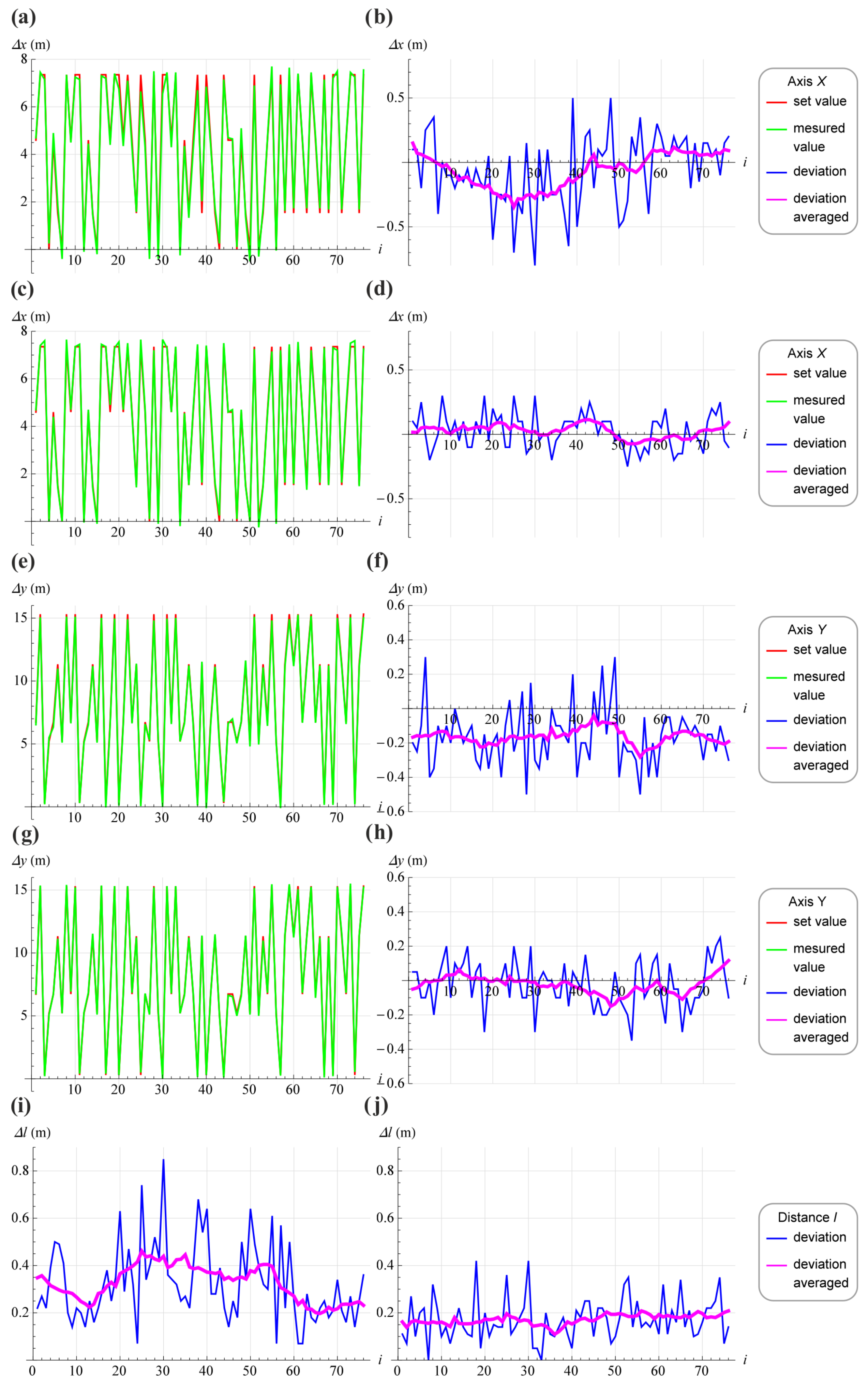
Figure 1. A mobile a vehicle with vision system on the test track. In the background, there is shown ARTag with coded number 10.
Applsci 11 04496 g001
Figure 2. Block diagram of the construction of a mobile vehicle.
Applsci 11 04496 g002
Figure 3. A photograph the vehicle with the implemented autonomous system.
Applsci 11 04496 g003
Figure 4. Determination scheme of position correction vector when one marker is detected.
Applsci 11 04496 g004
Figure 5. Determination scheme of position correction vector when two markers are detected.
Applsci 11 04496 g005
Figure 6. Determination scheme of position correction vector when three markers are detected.
Applsci 11 04496 g006
Figure 7. General overview of laboratory test environment.
Applsci 11 04496 g007
Figure 8. Accuracy measurement of the first control point. (a) Green points represent measured positions when the robot was standing still. The red point is an aim point. In this experiment, the robot had the vision system turned off. (b) The robot had the vision system turned on. (c) Deviations from the aim point in x and y, the vision system was off. (d) Deviations from the point where vision system was on.
Applsci 11 04496 g008
Figure 9. Accuracy measurement of point 2. (a) Green points represent measured positions when the robot stops. The red point is an aim point. In this experiment, the robot had a vision system turned off. (b) The robot had the vision system turned on. (c) Deviations from the aim point in x and y, where the vision system was off. (d) Deviations from the point where cameras the vision system was on.
Applsci 11 04496 g009
Figure 10. Accuracy measurement of point 3.(a) Green points represent measured positions when the robot stops. The red point is an aim point. In this experiment, the robot had thre vision system turned off. (b) The robot had the vision system turned on. (c) Deviations from the aim point in x and y, where the vision system was off. (d) Deviations from the point where the vision system was on.
Applsci 11 04496 g010
Figure 11. Accuracy measurement of point 4. (a) Green points represent measured positions when the robot stops. The red point is an aim point. In this experiment, the robot had the vision system turned off. (b) The robot had the vision system turned on. (c) Deviations from the aim point in x and y, where the vision system was off. (d) Deviations from the point where the vision system was on.
Applsci 11 04496 g011
Figure 12. Accuracy measurement of point 5. (a) Green points represent measured positions when the robot stops. The red point is an aim point. In this experiment, the robot had the vision system turned off. (b) The robot had the vision system turned on. (c) Deviations from the aim point in x and y, where the vision system was off. (d) Deviations from the point where cameras the vision system was on.
Applsci 11 04496 g012
Figure 13. Accuracy measurement in every 76 attempts, where the robots reached the aim point. (a,e) Differences between set (red) and reached (green) positions in x and y directions, when the vision system was off. (c,g) In those graphs the vison system was turned on. (b,f) Point deviations and average line (pink) in x and y directions, where the vision system was turned off. (d,h) The vision system was turned on. (i,j) Shows position inaccuracies, respectively with the vision system off and on.
Applsci 11 04496 g013
Figure 14. Software screenshot presenting the real position of the robot in test track.
Applsci 11 04496 g014
Figure 15. A mobile vehicle with a vision system on the test track. The red arrows point places where the vision system corrected the vehicle positions. The brown line is the path of the vehicle.
Applsci 11 04496 g015
Table 1. The quantitative results comparison of positioning accuracy without and with cameras.
Vision Sys. Turned OffVision Sys. Turned On
Sum of x module deviations17.308.55
Sum of y module deviations15.408.50
Sum of the distance module deviations24.7213.01
Publisher’s Note: MDPI stays neutral with regard to jurisdictional claims in published maps and institutional affiliations.

