Semantic Structure from Motion for Railroad Bridges Using Deep Learning

Abstract

Current maintenance practices consume significant time, cost, and manpower. Thus, a new technique for maintenance is required. Construction information technologies, including building information modeling (BIM), have recently been applied to the field to carry out systematic and productive planning, design, construction, and maintenance. Although BIM is increasingly being applied to new structures, its application to existing structures has been limited. To apply BIM to an existing structure, a three-dimensional (3D) model of the structure that accurately represents the as-is status should be constructed and each structural component should be specified manually. This study proposes a method that constructs a 3D model and specifies the structural component automatically using photographic data with a camera installed on an unmanned aerial vehicle. This procedure is referred to as semantic structure from motion because it constructs a 3D point cloud model together with semantic information. A validation test was carried out on a railroad bridge to validate the performance of the proposed system. The average precision, intersection over union, and BF scores were 80.87%, 66.66%, and 56.33%, respectively. The proposed method could improve the current scan-to-BIM procedure by generating the as-is 3D point cloud model by specifying the structural component automatically.

1. Introduction

Civil infrastructures such as roads, railroads, and bridges have an important role in human activities. Thus, it is important to ensure that they last a long time through proper maintenance. The current maintenance practice uses manpower to inspect the exterior of the structure and check for damage, deterioration, and erosion of the structure. Manual inspection is ineffective in terms of time, cost, and need for manpower. Thus, techniques that can improve the current maintenance practice are being introduced.

Recent developments in information technology (IT) have influenced the civil engineering domain, including the maintenance field. In particular, numerous studies have been carried out to replace the exterior survey dependent on manpower in the prior maintenance techniques through sensors or images. Yoon et al. [1] carried out health monitoring of structures using drones and imaging equipment. Cha et al. [2] carried out a study to automatically discriminate cracks on concrete surfaces using artificial intelligence. Narazaki et al. [3] reported automatic recognition of structural elements using artificial intelligence. Lee et al. [4] automatically extracted bridge design parameters based on point cloud data (PCD). Park et al. [5] predicted the dynamic characteristics of structures using image data.

Building information modeling (BIM) has recently been integrated into the field to conduct systematic and effective structure planning, design, construction, and maintenance. In Korea, a BIM guideline, “BIM application guide for architecture”, has been established, required for all projects with a total construction cost over 50 million dollars [6]. In addition, BIM was used to increase the productivity and reduce costs in projects such as the Admiralty Station project in Hong Kong, Danjiang Bridge project in Taiwan, and Zaha Hadid Architects project in the UK [7].

Although the BIM technique is increasingly being applied to newly planned structures, there are many difficulties in applying BIM to existing structures. Various studies have been carried out to apply BIM to existing structures [8,9,10,11,12,13,14,15]. Most of these techniques begin by generating a three-dimensional (3D) model of the structure. However, drawings may not exist for some structures, particularly old structures, when the drawings were not archived digitally. Furthermore, even if there is a design drawing, the current structure can be different from the drawing owing to deterioration, construction errors, etc. Therefore, to generate the as-is model of the structure, 3D PCD are obtained by either using light detection and ranging (LiDAR) or applying photogrammetry with images of the structure.

LiDAR can accurately produce a 3D point cloud model of a structure by emitting laser pulses and measuring the distance to the object by receiving the light reflected back from the target object. LiDAR is usually installed near the structure, which not only requires the operation of the facility to be stopped, but also is time-consuming and expensive. On the other hand, photogrammetry collects photographic data using a camera and generates 3D PCD by applying a 3D modeling technique such as Structure from Motion (SfM) [16]. The photogrammetry method requires less manpower and is less expensive than LiDAR. Photogrammetry has a lower accuracy than those of LiDAR systems but is improved with the recent advances in unmanned aerial vehicles (UAVs) and camera technologies.

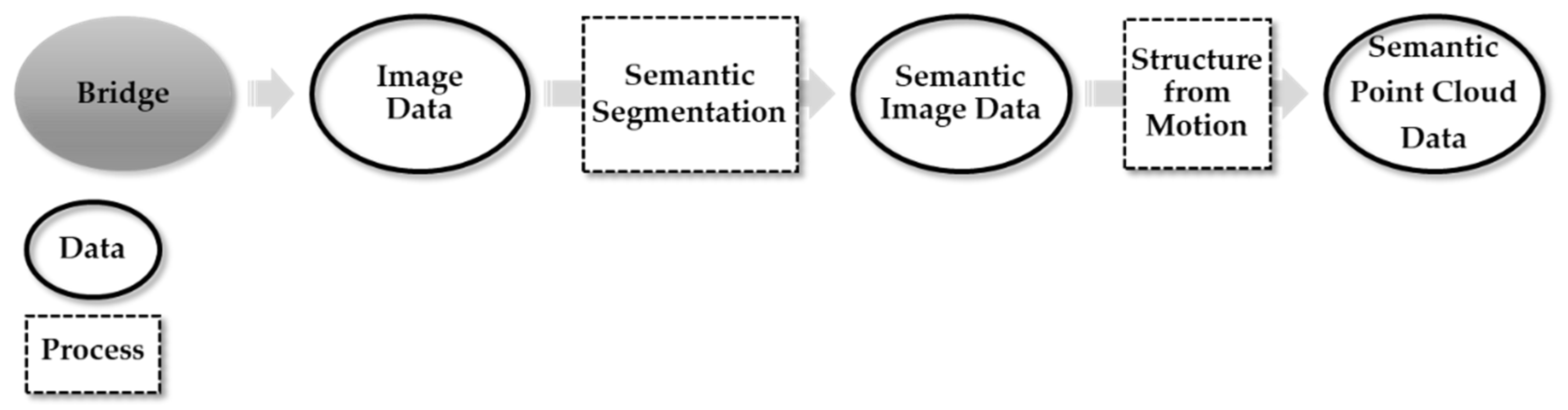
Therefore, this study aims to develop a semantic structure from motion (SSfM) method that collects photographic data and automatically assigns the structural component using a camera installed on an UAV. The proposed method utilizes a deep-learning-based semantic segmentation technique together with SfM to automatically classify the bridge component in a reconstructed 3D point cloud model. The proposed system consists of two steps, (1) semantic segmentation, which classifies every pixel in the bridge image into a structural component, and (2) SfM, which generates 3D PCD using the results of semantic segmentation. A detailed explanation of the proposed system, validation test, and discussion are presented.

2. Background

Computer vision, a field that enables computers to recognize and analyze visual information, has been continuously developed [17,18,19,20,21]. Deep learning techniques have recently introduced numerous applications in computer vision [22,23,24]. In particular, a convolutional neural network (CNN), which is one of the methods to classify images automatically, has been introduced in an image recognition contest “ImageNet Large-Scale Visual Recognition Challenge (ILSVRC)”, held in 2012. This study used a CNN-based semantic segmentation algorithm, Deeplab-V3+ [25], to classify each image pixel into a bridge component.

2.1. Semantic Segmentation Using Deep Learning

Semantic segmentation is a method of predicting and displaying the semantic information of an image by segmenting an image into pixels using a CNN. The general structure of a CNN is shown in Figure 1. The CNN extracts a convolution feature using the convolution layer and pooling layer alternately from the image (input data) and classifies the extracted features using a fully connected layer.

In this study, semantic segmentation was carried out using Deeplab-V3+. The structure of the Deeplab-V3+ model is shown in Figure 2. Deeplab-V3+ separates the structure into an encoder and decoder to overcome the disadvantage of the CNN, which loses location information owing to the loss of dimensions while passing the fully connected layer. The encoder extracts features at random resolution through atrous convolution from a deep convolutional neural network (DCNN). The output stride, which refers to the ratio of the resolution of the input image to the resolution of the output image, was applied. The decoder reduces the channel by performing a 1 × 1 convolution on the final output image of the encoder and performs concat after a bilinear upsample. Through the above process, the decoder efficiently maintains the object segmentation details [25].

Deeplab-V3+ has the advantage of using a pretrained deep learning model. In this study, ResNet-50 was used as a module together with Deeplab-V3+. ResNet-50 is a module using the proposed residual learning to address the gradient loss. In this phenomenon, a variable disappears as it passes a layer. The structure of the existing convolution layer and residual learning is shown in Figure 3.

Residual learning is the addition of a residual connection (or skip connection) to a prior convolution layer. It is composed of the addition of an input to the stack of two convolution layers. Figure 3a describes the structure of the existing CNN. Back-propagation training is performed to obtain a weight that minimizes the difference between the predicted value (H(x)) of the network and target value (label) of the training data. The predicted value H(x) refers to the result of learning the network through data. The target value refers to a label matching the training data. Figure 3b shows the structure of the residual learning block of ResNet-50. The purpose of learning is F(x) becoming 0, considering the hypothesis that it is better to approximate F(x) + x to H(x) than to approximate H(x) as a function of a complex nonlinear structure. In other words, when H(x) ≃ F(x) + x, it changes to F(x) ≃ H(x)–x, and eventually learning F(x) is the output factor H(x) and the input factor x is to learn the difference. Therefore, it can be considered that the residual that is the remainder is learned. Finally, the meaning of learning the optimal F(x) is the same as that of the convergence of F(x) to 0; as x becomes a residual connection (or skip connection), there is no increase in the amount of computation [26].

2.2. SfM

SfM is one of the most popular methods for generation of a 3D model using image data [27,28,29]. The first step in SfM is to identify the correspondence between the images. SfM uses scale-invariant feature transform (SIFT) and speeded-up robust feature (SURF) algorithms to find feature points in photographic data and identify correspondence between feature points [30,31]. However, not all of the obtained feature points belong to a correspondence relationship. An outlier in which the feature points do not coincide can exist. In SfM, random sample consensus (RANSAC) was used, which is a method of randomly selecting sample data to remove outliers and selecting data with the largest consensus. As shown in Figure 4, a feature model of each photograph was obtained by applying RANSAC and a feature matching process was performed to compare the feature models. In this process, if the points match through feature matching, it is determined as a correspondence relationship; if not, it is regarded as an outlier and removed.

When the correspondence between the pictures is grasped through the above process, the position of the camera can be estimated, and the feature points can be expressed as 3D PCD. However, it is not possible to express all shapes of an object with 3D PCD generated only with feature points. Therefore, the 3D dense reconstruction technique is used to obtain dense 3D PCD. The 3D dense reconstruction technique is a method of interpolation using pixels around feature points. Normalized cross correlation (NCC) and inverse distance weighted techniques are used.

NCC is a technique for measurement of geometric similarity by comparing the red–green–blue (RGB) values of pixels. The 3D dense reconstruction technique refers to the surrounding pixels of the feature point. The RGB value of the surrounding pixels is extracted using a filter on the pixel size. If the RGB obtained from the 3D dense reconstruction technique is calculated using Equation (1), the NCC can be obtained.

$$\frac{1}{n}{\displaystyle \sum }_{x,y}\frac{\left(f\left(x,y\right)-\overline{f}\right)\left(t\left(x,y\right)-\overline{t}\right)}{{\sigma }_f{\sigma }_t}$$

(1)

where n is the size of the filter, f(x,y) is the RGB at the coordinates of the filter, t(x,y) is the RGB at the x and y coordinates of the comparison filter, $\overline{f}$ is the average RGB of the filter, $\overline{t}$ is the average RGB of the comparison filter, ${\sigma }_f$ is the standard deviation of the RGB of the filter, and ${\sigma }_t$ is the standard deviation of the RGB of the comparison filter. As the RGB is nonnegative, NCC has a value between −1 and 1. If NCC is close to 1, the two filters are similar. However, because the NCC obtained from the process does not include the distance information of the photograph, a high reliability cannot be ensured. Therefore, the process of assigning a weight to a distance is required. The NCC uses the inverse distance weighting method, expressed by

$$Z_p=\frac{{{\displaystyle \sum }}_{i=1}^n{Z}_i{W}_i}{{{\displaystyle \sum }}_{i=1}^n{W}_i}$$

(2)

where $Z_p$ is the estimated value (interpolation value) of the estimation point, $Z_i$ is the reference value of the position ($x_i$, $y_i$), $W_i$ is the weight, and n is the number of reference values. The weight $W_i$ can be calculated using Equation (3), where $d_i$ represents the distance,

$$W_i=\frac{1}{d_i^2}$$

(3)

Through this process, interpolation is performed on a section in which no feature point exists, and dense 3D PCD can be generated based on the result.

3. System Development

This study developed an SSfM that automatically classifies image pixels into bridge components using deep learning and generates a 3D point cloud model while preserving the information on bridge components such as piers and girders. Figure 5 shows an overview of the proposed system. The contents of each component are described in detail.

3.1. Bridge Component Classification Using Semantic Segmentation

The first step of the proposed system is to provide semantic information of the bridge components to each pixel in the two-dimensional (2D) images. In this study, information on bridge components was assigned by performing transfer learning based on Deeplab-V3+. Transfer learning is a method of constructing a network using a pretrained deep learning model. Transfer learning can result in a high accuracy using a pretrained deep learning model with a high performance. In this study, transfer learning was performed using Deeplab-V3+/ResNet-50 and a network was developed to classify the components of the bridge. The network developed in this study classified each pixel of the image into 10 classes: pole, building, girder, pier, ground, grass, water, sky, car, and road. Eight classes, except girder and pier, which are components of the bridge, were integrated into the background later. A total of 245 photographic data with a resolution of 800 × 600 pixels were used as the training data. Among the 245 images, 103 were collected through Google Street View, while 142 images were obtained using unmanned aerial images at the Osong 5th Test track bridge in Nojang-ri, Jeon-myeon, and Sejong. The equipment for unmanned aerial photography included DJI Inspire 2 and Zenmuse X5S, as shown in Figure 6. The specifications of the equipment are listed in

Table 1. Specification of Inspire 2.

Maximum speed	94 km/h
Maximum flight time	Approximately 27 min
Maximum service ceiling above sea level	2500 m
Maximum tilt angle	35°
Hovering accuracy (P mode)	Vertical: 0.1 m/Horizontal: 0.3 m
Weight	3440 g

and

Table 2. Specification of Zenmuse X5S.

Lens	DJI MFT 15 mm/1.7 ASPH
Image sensor	CMOS, 4/3
Focal length	15 mm
Image resolution	5280 × 3956
Field of view	72°
Weight	461 g

.

To train the semantic segmentation network, a labeling process is required to designate which component information of a bridge is contained in each pixel of a photograph. In this study, pixel label data were generated using MATLAB Image Labeler. The label has 10 classes: pole, building, girder, pier, ground, grass, water, sky, car, and road. Figure 7 and Figure 8 show the photographic data and label data used for learning. In addition, the number of pixels for each class was used as a weight to balance the classes.

The Holdout method was used, as shown in Figure 9, for network learning and verification. For the training data, 80% of the 245 data obtained with the Osong 5th test track and Google street view were randomly selected. The remaining 20% of the data were used for network self-validation. The hyperparameters used for the training are listed in

Table 3. Hyperparameters.

Batch size	5
Epoch number	500
Optimizer	Adam optimizer
Initial learn rate	0.001
Learn rate drop period	10
Learn rate drop factor	0.3

. The batch size was set to 5, while the epoch number was set to 500. The Adam optimizer was used for optimization. The initial learning rate was 0.001. The epoch number was reduced 0.3 times every 10 times. The configuration of the deep learning network used for training is shown in Figure 10.

3.2. Construction of 3D PCD Using SfM

The trained network classifies images into 10 classes, including bridge components. Eight classes that are not bridge components were integrated into the background, resulting in three classes: girder, pier, and background. The bridge components classified using the above method are in 2D images and not in a 3D point cloud model. To convert the semantic information from a 2D image to a 3D point cloud model, an SfM technique, as shown in Figure 11, was applied.

The SfM technique, which generates a 3D point cloud model using 2D images, finds location and geometry information by utilizing key points common in several images. Key points are matched from SIFT using image intensity information. In this study, a method of overlaying label data, semantic information on photography data, was used to reflect both location information and semantic information. The key point was found using the intensity information of the original photography data. 3D location information was obtained for each pixel of the image. After finding the location information, the semantic information was transformed to an RGB value and visualized with a transparency of 50% over the original image data. Through this process, it was possible to visualize the 3D PCD of the bridge together with the bridge component information.

4. Validation Test

To verify the performance of the proposed SSfM system, an experiment was carried out using the test data collected from the Osong 3rd test track in Osong-eup, Heungdeok-gu, Cheongju-si, Chungcheongbuk-do, Korea. A total of 183 test data were collected from the Osong 3rd test track using drones as test data and the semantic segmentation technique developed in this study was applied to automatically classify the components of the bridge. In addition, SfM was applied based on 183 images with semantic information and a 3D point cloud model including information on the components of the bridge was obtained.

In general, a confusion matrix, as shown in

Table 4. Confusion matrix.

		Predicted Class
		True	False
Actual class	True	True positive (TP)	False negative (FN)
	False	False positive (FP)	True negative (TN)

, was used to evaluate the result of semantic segmentation. Measures to evaluate using the error matrix include accuracy, intersection over union (IoU), precision, recall, and F1 score.

Accuracy is one of the measures used to intuitively evaluate the performance of a classification model, as shown in Equation (4). However, data with unbalanced results can distort the performance of the model and must be expressed using other methods.

$$Accuracy=\frac{TP+TN}{TP+FP+FN+TN}$$

(4)

IoU is an intuitive measure for the evaluation of the performance of a classification model as an intersection. It is most often used to evaluate the prediction results in semantic segmentation and object detection,

$$IoU=\frac{TP}{FN+TP+FP}$$

(5)

Precision and recall are usually used together and exhibit an inverse relationship. However, both measures have drawbacks, so that they are used together in the F1 score. The F1 score is an index representing the harmonic average of precision and recall and can accurately evaluate the performance of the model even with unbalanced data. Precision, recall, and F1 scores (denoted BF) are defined in Equations (6)–(8), respectively.

$$\mathit{Precision}=\frac{TP}{TP+FP}$$

(6)

$$Recall=\frac{TP}{TP+FN}$$

(7)

$$F1\mathit{score}=2\times \frac{\mathit{Precision}\times Recall}{\mathit{Precision}+Recall}$$

(8)

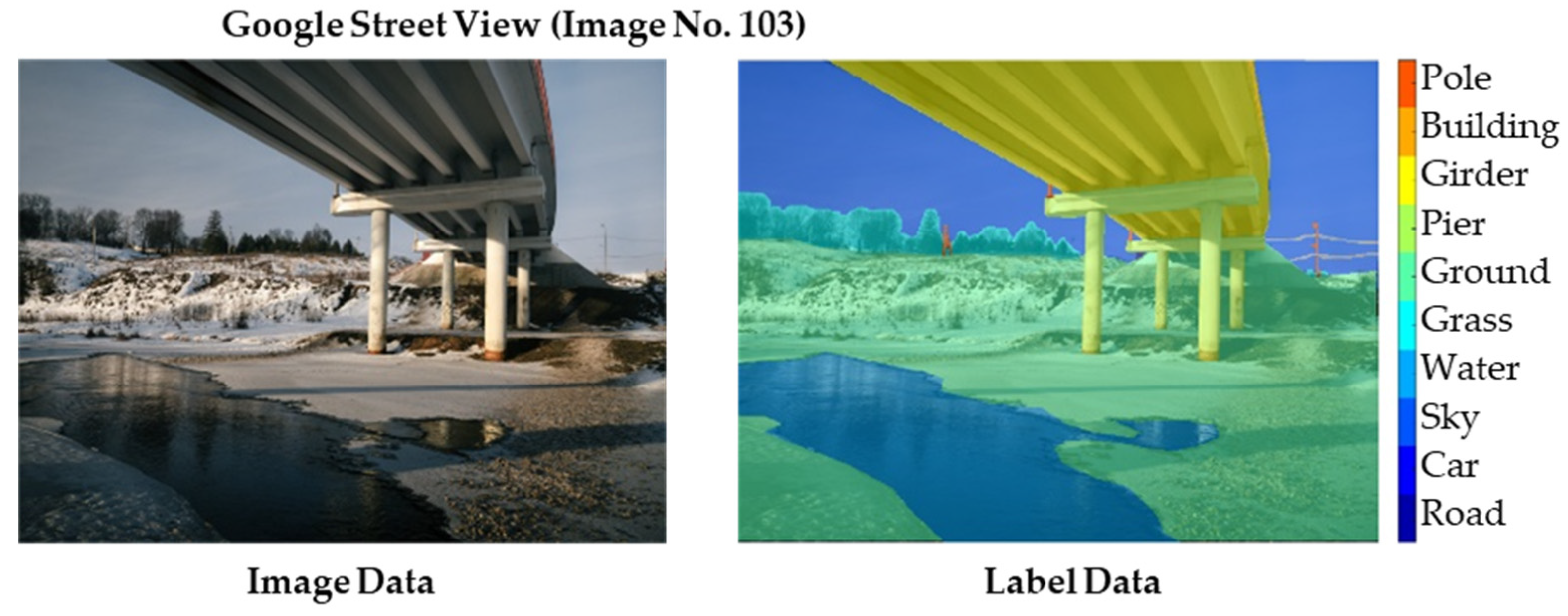
The proposed semantic segmentation network classified 183 test data collected from the Osong 3rd test track. The results are shown in Figure 12 and

Table 5. Semantic segmentation results.

	Class
	Girder	Pier	Average
Accuracy (%)	85.00	76.73	80.87
IoU (%)	80.22	53.09	66.66
BF-score (%)	62.49	50.17	56.33

. The bridge component classification network proposed in this study was able to automatically classify the girder and pier on the image, with an average accuracy of approximately 80%, IoU of 66%, and BF-score of approximately 56%.

After the application of 183 data to the bridge component classification network, 3D PCD were generated by applying SfM. The results are shown in Figure 13 and

Table 6. SSfM results.

	Class
	Girder	Pier	Average
Precision (%)	78.64	69.81	74.23
IoU (%)	75.05	56.74	65.90
BF-score (%)	59.29	51.88	55.59

. The results of semantic segmentation could be successfully expressed in the 3D point cloud model. The average precision was approximately 74%, the IoU was approximately 65%, and the BF-score was approximately 55%. It was expected that an additional error will occur in SfM, which converts 2D images to a 3D point cloud model, resulting in lower SfM results than the 2D segmentation results. However, as the semantic segmentation results of several images were averaged to a 3D point of one, the IoU and BF-score of a specific class (pier) slightly increased.

5. Conclusions and Discussion

In this study, an automatic procedure for generation of a 3D point cloud model that contains bridge component information was proposed using deep learning and computer vision. The verification test was carried out at the Osong 3rd test track located in Osong-eup, Heungdeok-gu, Cheongju-si, Korea, by applying the proposed technique to the collected images. The proposed method was able to automatically generate a 3D point cloud model containing information on bridge components with an accuracy of 74.23%, IoU of 65.90%, and average BF score of 55.59%.

Lee et al. [4] conducted a study to automatically extract design parameters of bridges using 3D Point Cloud Data, and the results showed high reliability. However, this study used LiDAR to acquire 3D Point Cloud Data. There is a problem where the bridge must be shut down in order to obtain 3D point cloud data from LiDAR. In order to solve this problem, in this study was conducted to collect 2D image data with an unmanned aerial and generate 3D point cloud data using the 2D image data.

It was confirmed that the proposed method in this study has a problem of increasing the error because errors are accumulated in the process of SSfM. However, if errors are minimized in the future by using deep learning models with improved modulus and big data, it is expected that time and cost in the modeling for the BIM of existing structures can be saved.

References

1. Yoon, H.; Elanwar, H.; Choi, H.; Golparvar-Fard, M.; Spencer Jr, B.F. Target-free approach for vision-based structural system identification using consumer-grade cameras. Struct. Control Health Monitor. 2016, 23, 1405–1416. [Google Scholar] [CrossRef]
2. Cha, Y.-J.; Choi, W.; Büyüköztürk, O. Deep learning-based crack damage detection using convolutional neural networks. Comput. Aided Civ. Infrastruct. Eng. 2017, 32, 361–378. [Google Scholar] [CrossRef]
3. Narazaki, Y.; Hoskere, V.; Hoang, T.A.; Fujino, Y.; Sakurai, A.; Spencer, B.F., Jr. Vision-based automated bridge component recognition with high-level scene consistency. Comput. Aided Civ. Infrastruct. Eng. 2020, 35, 465–482. [Google Scholar] [CrossRef]
4. Lee, J.H.; Park, J.J.; Yoon, H. Automatic bridge design parameter extraction for scan-to-BIM. Appl. Sci. 2020, 10, 7346. [Google Scholar] [CrossRef]
5. Park, G.; Hong, K.-N.; Yoon, H. Vision-based structural FE model updating using genetic algorithm. Appl. Sci. 2021, 11, 1622. [Google Scholar] [CrossRef]
6. Park, T.S.; Park, H.S. The current status and facilitation strategy of BIM for civil infrastructure projects. J. Korean Soc. Civ. Eng. 2018, 38, 133–140. [Google Scholar]
7. Kim, S.-W. Overseas BIM cases and effective use method of BIM. Railw. J. 2018, 21, 129–135. [Google Scholar]
8. Ilter, D.; Ergen, E. BIM for building refurbishment and maintenance: Current status and research directions. Struct. Surv. 2015, 33, 228–256. [Google Scholar] [CrossRef]
9. Bosché, F.; Ahmed, M.; Turkan, Y.; Haas, C.T.; Haas, R. The value of integrating scan-to-BIM and scan-vs-BIM techniques for construction monitoring using laser scanning and BIM: The case of cylindrical MEP components. Autom. Constr. 2015, 49, 201–213. [Google Scholar] [CrossRef]
10. Wang, Q.; Guo, J.; Kim, M.-K. An application oriented scan-to-BIM framework. Remote Sens. 2019, 11, 365. [Google Scholar] [CrossRef] [Green Version]
11. Bao, S.Y.; Savarese, S. Semantic Structure from Motion. In Proceedings of the CVPR 2011, IEEE, Colorado Springs, CO, USA, 20–25 June 2011; pp. 2025–2032. [Google Scholar]
12. Abbondati, F.; Biancardo, S.A.; Palazzo, S.; Capaldo, F.S.; Viscione, N. I-BIM for existing airport infrastructures. Transp. Res. Proc. 2020, 45, 596–603. [Google Scholar] [CrossRef]
13. Biancardo, S.A.; Viscione, N.; Oreto, C.; Veropalumbo, R.; Abbondati, F. BIM Approach for Modeling Airports Terminal Expansion. Infrastructures 2020, 5, 41. [Google Scholar] [CrossRef]
14. Abbondati, F.; Biancardo, S.A.; Sicignano, G.; De Oliveira, S.G.; Tibaut, A.; Dell’Acqua, G. BIM Parametric Modelling of a Railway Underpass. Ingegneria Ferroviaria 2020, 6, 443–459. [Google Scholar]
15. Abbondati, F.; Oreto, C.; Viscione, N.; Biancardo, S.A. Rural Road Reverse Engineering Using BIM: An Italian Case Study. In Proceeding of the International Conference on Environmental Engineering, Vilnius, Lithuania, 1–2 August 2020; Volume 11, pp. 1–7. [Google Scholar]
16. Ullman, S. The interpretation of structure from motion. Proc. R. Soc. Lond. Ser. B Biol. Sci. 1979, 203, 405–426. [Google Scholar]
17. Jiang, R.; Jáuregui, D.V.; White, K.R. Close-range photogrammetry applications in bridge measurement: Literature review. Measurement 2008, 41, 823–834. [Google Scholar] [CrossRef]
18. Kwiatkowski, J.; Anigacz, W.; Beben, D. Comparison of Non-Destructive Techniques for Technological Bridge Deflection Testing. Materials 2020, 13, 1908. [Google Scholar] [CrossRef]
19. Gawronek, P.; Makuch, M.; Mitka, B.; Gargula, T. Measurements of the Vertical Displacements of a Railway Bridge Using TLS Technology in the Context of the Upgrade of the Polish Railway Transport. Sensors 2019, 19, 4275. [Google Scholar] [CrossRef] [Green Version]
20. Kwiatkowski, J.; Anigacz, W.; Beben, D. A Case Study on the Noncontact Inventory of the Oldest European Cast-iron Bridge Using Terrestrial Laser Scanning and Photogrammetric Techniques. Remote Sens. 2020, 12, 2745. [Google Scholar] [CrossRef]
21. Porras-Amores, C.; Mazarrón, F.R.; Cañas, I.; Villoria Sáez, P. Terrestrial Laser Scanning Digitalization in Underground Constructions. J. Cult. Herit. 2019, 38, 213–220. [Google Scholar] [CrossRef]
22. Kim, H.; Yoon, J.; Sim, S.-H. Automated Bridge Component Recognition from Point Clouds Using Deep Learning. Struct. Control Health Monit. 2020, 27, e2591. [Google Scholar] [CrossRef]
23. Liang, X. Image-based Post-Disaster Inspection of Reinforced Concrete Bridge Systems Using Deep Learning with Bayesian Optimization. Comput. Aided Civ. Infrastruct. Eng. 2019, 34, 415–430. [Google Scholar] [CrossRef]
24. Krizhevsky, A.; Sutskever, I.; Hinton, G.E. Imagenet Classification with Deep Convolutional Neural Networks. Adv. Ineural Inf. Process. Syst. 2012, 25, 1097–1105. [Google Scholar] [CrossRef]
25. Chen, L.-C.; Zhu, Y.; Papandreou, G.; Schroff, F.; Adam, H. Encoder–Decoder with Atrous Separable Convolution for Semantic Image Segmentation. In Proceedings of the European Conference on Computer Vision, Munich, Germany, 8–14 September 2018; pp. 801–818. [Google Scholar]
26. Sin, H.J.; Yang, J.S.; Song, T.S.; Kwak, N.J. Network analysis according to modified architecture of residual block of ResNet. Korean Inst. Inf. Commun. Eng. 2019, 10, 292–294. [Google Scholar]
27. Moghaddam, B.; Lee, J.; Pfister, H.; Machiraju, R. Model-Based 3D Face Capture with Shape-from-Silhouettes. In Proceedings of the 2003 IEEE International SOI Conference. (Cat. No. 03CH37443), Nice, France, 17 October 2003; pp. 20–27. [Google Scholar]
28. Hartley, R.; Zisserman, A. Multiple View Geometry in Computer Vision; Cambridge University Press: Cambridge, UK, 2003. [Google Scholar]
29. Amberg, B.; Blake, A.; Fitzgibbon, A.; Romdhani, S.; Vetter, T. Reconstructing High Quality Face-Surfaces Using Model Based Stereo. In Proceedings of the 2007 IEEE 11th International Conference on Computer Vision, Rio de Janeiro, Brazil, 14–21 October 2007; pp. 1–8. [Google Scholar]
30. Lowe, D.G. Object Recognition from Local Scale-Invariant Features. In Proceedings of the Seventh IEEE International Conference on Computer Vision, Kerkyra, Greece, 20–27 September 1999; Volume 2, pp. 1150–1157. [Google Scholar]
31. Bay, H.; Tuytelaars, T.; Van Gool, L. Surf: Speeded Up Robust Features. In European Conference on Computer Vision; Springer: Berlin/Heidelberg, Germany, 2006; pp. 404–417. [Google Scholar]
Figure 1. Structure of the CNN.
Applsci 11 04332 g001
Figure 2. Structure of Deeplab V3+.
Applsci 11 04332 g002
Figure 3. Original convolution layer and residual learning block. (a) Original convolution layer; (b) residual learning block.
Applsci 11 04332 g003
Figure 4. Feature matching.
Applsci 11 04332 g004
Figure 5. Overview of the proposed SSfM system.
Applsci 11 04332 g005
Figure 6. Unmanned aerial photography equipment. (a) DJI Inspire 2; (b) Zenmuse X5S.
Applsci 11 04332 g006aApplsci 11 04332 g006b
Figure 7. Google street view images and labels.
Applsci 11 04332 g007
Figure 8. Osong 5th test track bridge images and labels.
Applsci 11 04332 g008
Figure 9. Overview of the holdout method.
Applsci 11 04332 g009
Figure 10. Structure of Deeplab-V3+/ ResNet-50.
Applsci 11 04332 g010
Figure 11. Principle of the SfM photogrammetry.
Applsci 11 04332 g011
Figure 12. (a) Image data; (b) predicted label data.
Applsci 11 04332 g012
Figure 13. Semantic PCD of the Osong 3rd test track bridge.
Applsci 11 04332 g013