Parametric Study of the Corrosion of API-5L-X65 QT Steel Using Potentiostat Based Measurements in a Flow Loop

Abstract

Low-carbon steel is widely used in industrial pipelines, and corrosion studies are focused mostly on erosion-corrosion, its prediction and control. In this paper, the corrosion rate in pipelines is modeled using a flow loop and measured by linear polarization resistance method (LPR) using a 3-electrode corrosion setup for API-5L-X65 QT steel. Optical microscopy and SEM studies are conducted to examine the surface of the sample and the corrosion products. The effect of NaCl concentration on the corrosion rate is studied at different pH, temperature range, and flow velocities with dissolved oxygen content in the solution maintained at 6 mg/L (6ppm). The corrosion rate is found to be varying from 1 mil per year (0.0254 mmyr⁻¹) to 10 mils per year (0.254 mmyr⁻¹), and the corrosion rate increases with the flow velocity and reaches a maximum at Reynolds Number above 10,000. Further increase in fluid velocity shows corrosion is flow insensitive, and uniform corrosion is predominant in the region.

1. Introduction

Corrosion is a natural phenomenon associated with metals that leads to material destruction. Corrosion is an engineering problem, as well as an economic problem as the financial losses associated with corrosion, is enormous. The cost of corrosion worldwide in 2017 [1] was shown to be approximately 3.4% of the global GDP ($2.5 trillion). The same published study showed the cost of corrosion in the US to be 3.1% of GDP ($276 billion). In India, the cost of corrosion was estimated as 2.4% of the GDP in 2011-12 [2]. Pipeline accidents, due to corrosion, are frequent in the oil and gas industries. A study conducted by Saudi Aramco in 2013 concluded that the cost of corrosion for their operations was around $900 million per year [3]. Corrosion is not completely avoidable, so the industry needs to find ways to monitor, control, mitigate, and reduce corrosion. Implementing a proper corrosion management approach in the industry requires an in-depth understanding of corrosion mechanisms and implementing reliable methods to assess the corrosion rate [4].

Corrosion assisted by flow causes severe damages to oil and gas pipelines, heat exchanger systems in process industries. Maintenance and replacement of these corroded components are very expensive. The corrosion rates depend upon many factors, such as dissolved oxygen concentration, temperature, total dissolved salts, pH, fluid dynamics, and presence of scale on internal surfaces [5]. H.R Copson [6], in his studies summarizes that the corrosion assisted by flow varies according to the material under investigation and with the exposure conditions. He also states that flow generally increases the corrosion rates, but in some special cases, the effect can be the opposite. Rotating disk electrode method and impingement jet systems are two conventional methods used to measure the corrosion rates in a flow system. In the work of Namboodhiri et al. [7], a correlation between mass transfer and flow is developed using the rotating cylinder method to evaluate the corrosion of High Strength Low Alloy (HSLA) steel in 3.5% NaCl solution. However, it is not always possible to reproduce the exact flow patterns occurring in the pipeline system in the rotating cylinder device. A flow loop system provides a more realistic environment to evaluate the actual corrosion rates in a pipeline system [8].

The corrosion rate of steel in a flow loop system can be estimated using weight loss methods, electrochemical methods, and other methods, such as corrosion characterization, and acoustic emission measurements. Y. Utanohara et al. [9] investigated the corrosion rate at a pipe elbow using the electric resistance method to study the effect of the thermal flow field on corrosion rates. The corrosion rates were measured at a temperature range of 50–150 °C and flow velocities of 0–6 m/s, and the corrosion rate was found to have a nonlinear relationship with velocity [9]. Temperature and fluid velocity were the only two parameters that varied. Weight loss methods give an average corrosion rate over a period of time, but the measuring process takes a long time. The great difficulty with the weight loss method is the ability to hold all process parameters constant for a long period of time to see the effect of one parameter on the corrosion rate.

For a pipeline, there are so many parameters that can affect its corrosion rate, each of which tends to have an exponential effect on the corrosion rate that most methods give poor and irreproducible results. Electrochemical techniques are ideal for the study of corrosion in pipelines—particularly the linear polarization resistance (LPR) method, since the measurement is rapid (less than 5 min), does not affect the sample, and can be automated to perform continuous measurement of corrosion rate. For this method to work, the material should be polarized typically on the order of ±10 mV compared to the Open Circuit potential, when there is no net current is flowing. By taking the slope of the potential versus current curve, as the current flow is induced between the working and counter electrodes [10] and using the Stern-Geary equation, the resistance can then be used to find the corrosion rate of the material. Corrosion rate measurements in the flow loop have been done by various researchers to evaluate the flow accelerated corrosion and erosion. Zafar et al. [11] used a flow loop to investigate the corrosion resistance of SA-543 and X65 steels in an oil-water emulsion containing H₂S and CO₂ using polarization curves. LPR was measured using a potentiostat and two-electrode system for 24hrs at an interval of 30 min. The effect of salt concentration and pH on corrosion rate was not considered in this work. Ajmal et al. [12] investigated the flow accelerated corrosion of oil field water in the loop system at pipe elbows at turbulent conditions using the LPR method and correlated the corrosion rates with fluid velocities and shear stresses, and the electrochemical results were validated using CFD simulation results. Huang et al. [13] used the polarization method to evaluate the corrosion behavior of X52 steel at an elbow of a loop system and its correlation with flow velocity, shear stress, and the volume fraction of particles. The work by Sun et al. [14] did a parametric study to evaluate the effects of CO₂ on corrosion rates of carbon steels (C1010, C1018, and X65) using a flow loop. Localized corrosion rates were determined at two temperatures (40 °C and 90 °C), pH, salt concentrations, flow regimes, and CO₂ partial pressure using the LPR method. In [14], the salt concentration was varied from 0 to 1%. The effect of flow rate on corrosion rate was not considered in this work, and the superficial gas and liquid velocities were assumed as 10 m/s and 0.1 m/s, respectively.

One of the earliest corrosion prediction models was by de Waard and Milliams [15] in 1975, where the authors studied the relationship between the corrosion rate on grit blasted steel specimens (X52) and partial pressure of CO₂. De Waard-Milliams provided a model to determine the corrosion rates incorporating the effects of pH and temperature. The relation was modified in his later works and provided a modified equation [16], which accounts for the effect of dissolved iron at lower and higher temperatures. Corrosion studies of 316 Stainless Steel were performed by Jepson et al. [17] using oil-water in a flow loop, and the rates were determined using electrical resistance probes and weight loss methods. The findings were used to develop a predictive equation for corrosion rates at different temperatures, flow velocities, and carbon dioxide partial pressure for the oil-water mixture. In recent works, the CO₂-multi-phase flow corrosion model is presented by Nesic et al. [18], which considers the kinetics of electrochemical reactions, diffusion effects, and the effect of steel type. The model also considers the kinetics of scale growth and precipitations and accounts for the effect of steel types, multi-phase flow, and H₂S. Nothing is mentioned of the steel types in the paper except they are mild steels. Pots [19] developed a corrosion prediction tool HYDROCOR, a computer-based engineering spreadsheet for localized corrosion in carbon pipelines considering various scenarios in the field. The model accounts for various environments with corroding agents like CO₂, H₂S, (organic) acids, bacteria, and oxygen, and the spreadsheet model is coupled with models for water chemistry, multi-phase flow, oil protectiveness, heat transfer, and thermodynamics using FORTAN to predict different scenarios. Khajotia et al. [20] used “a Case-based Reasoning-Taylor Series (CBR-TS) model” to predict the corrosion behavior in field pipelines considering operation parameters. Case-based reasoning model and Taylor expansion method are employed to predict the corrosion rate as a function of pipeline material, pH, CO_2, and H₂S content and temperature. The CBR-TS model was tested using a field database and a hypothetical database. NORSOK M-506 [21] developed a semi-empirical corrosion rate model using laboratory data that investigates the corrosion rates in a flow loop by varying parameters, such as temperature, solution pH, and CO₂ partial pressure, but it has limitations to predict the interaction between CO₂ and H₂S.

The aforementioned corrosion rate models do not include the interaction of chlorine ions and the corrosion effects. Whilst predictive software for pipeline corrosion is commercially available (11 commercial software packages), the results of each predictive package do not agree with each other. Even different versions of the same software have been known to give different corrosion rate results. There are many reasons for this, but it is clear that there is still a need for self-consistent predictive software for pipeline corrosion. 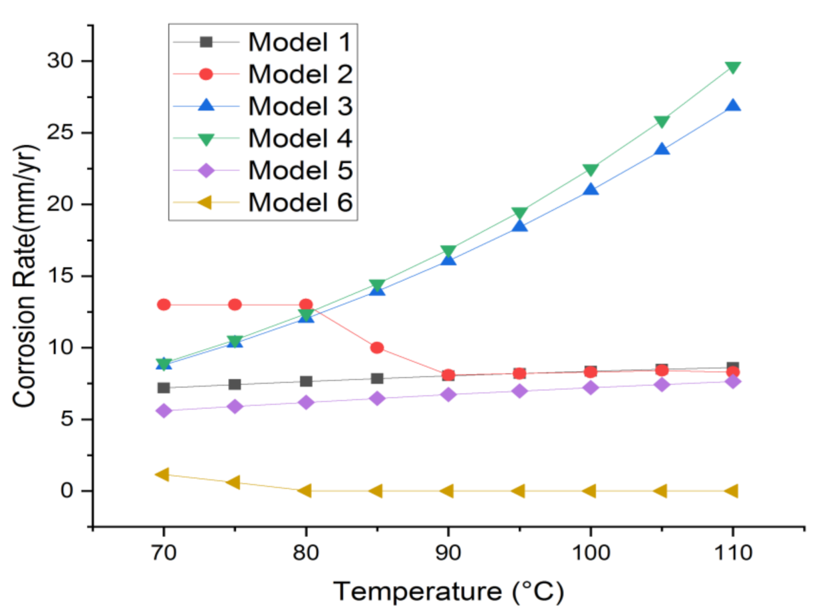Rolf Nyborg [22] has reviewed the models available to predict Corrosion rate in different CO₂ partial pressures, temperatures, and other flow parameters, and the work concludes that all the models have limitations depending upon the philosophy used in developing these models. A general prediction of the corrosion rates is difficult as the corrodents and the environmental factors are varying in different field data. The work concludes that the prediction of corrosion rates by these models vary considerably from case to case—most models are successful in predicting their respective data, but very unsuccessful when predicting other field data. This is concluded in Figure 1 below, where six different models are analyzed by our research team, which is similar to the comparison done by Nyborg in his work, and the results show a large deviation in corrosion prediction in all these models.

In the oil industries, the corrosion rates of pipelines are intensified when the hydrocarbons phase is transported with corrosive brines, and the composition and its effects should be analyzed to predict the rates [23]. The presence of NaCl complicates the kinetics and the mechanism of pipeline corrosion depending on whether it is deaerated or aerated systems. The effect of chloride ions on corrosion rates varies depending upon the environment as it affects anodic kinetics, scale formation, CO₂ solubility, and pH [24]. However, in the literature, there are limited studies that provide corrosion rate models with detailed parametric studies in NaCl solutions. To improve the prediction of corrosion rates a parametric study incorporating the different parameters which affect corrosion is desirable, especially in pipelines in the industries where the flow conditions and rates are not stable. In his later work, Nesic et al. updated his previous work [18] to develop an H₂S Corrosion model [25] which includes the kinetics of iron sulfide growth with experimental results at very low temperatures (5 °C to 20 °C) and high salinity brines (up to 25 wt% NaCl). In CO₂-saturated solutions, the effect of NaCl concentration on corrosion rates in carbon steel is studied by [26] exposing the sample for 100 h by changing NaCl concentrations from 0.001 wt% to 10 wt% at room temperature. The corrosion rates were determined using Electrochemical Impedance Spectroscopy (EIS) and linear polarization method under the freely corroding condition and authors also studied anodic and cathodic kinetics using microelectrode technique. According to this study, the corrosion rate tends to decrease with NaCl concentration, which is opposite to the naturally aerated seawater. The effect of NaCl concentration on mild steel in CO₂-saturated brines is studied by [24,27] using a mechanistic model that considers mass transfer and electrochemical kinetics. The corrosion rates predicted by the model is compared with corrosion rates obtained using experiments conducted in a deaerated, CO₂-saturated brine environment. The study was conducted using a three-electrode electrochemical glass cell, and the corrosion rates were measured using LPR and EIS techniques. The flow rates are changed by changing the stirrer speed from 100 to 800 rpm. The authors studied the effect of pCO₂, NaCl concentrations on corrosion rates of the mild steel, and the experimental results show corrosion rates are independent of flowrate at high salinity. The proposed model could not predict this flow insensitive behavior at high flow rates.

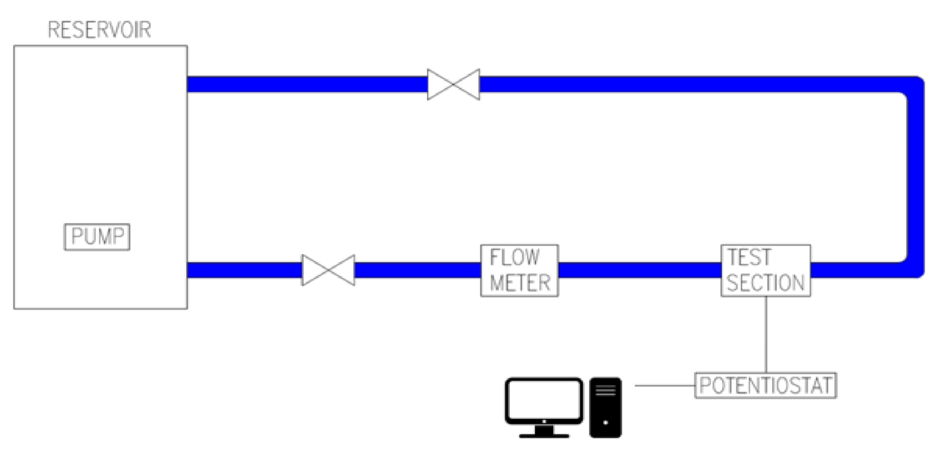
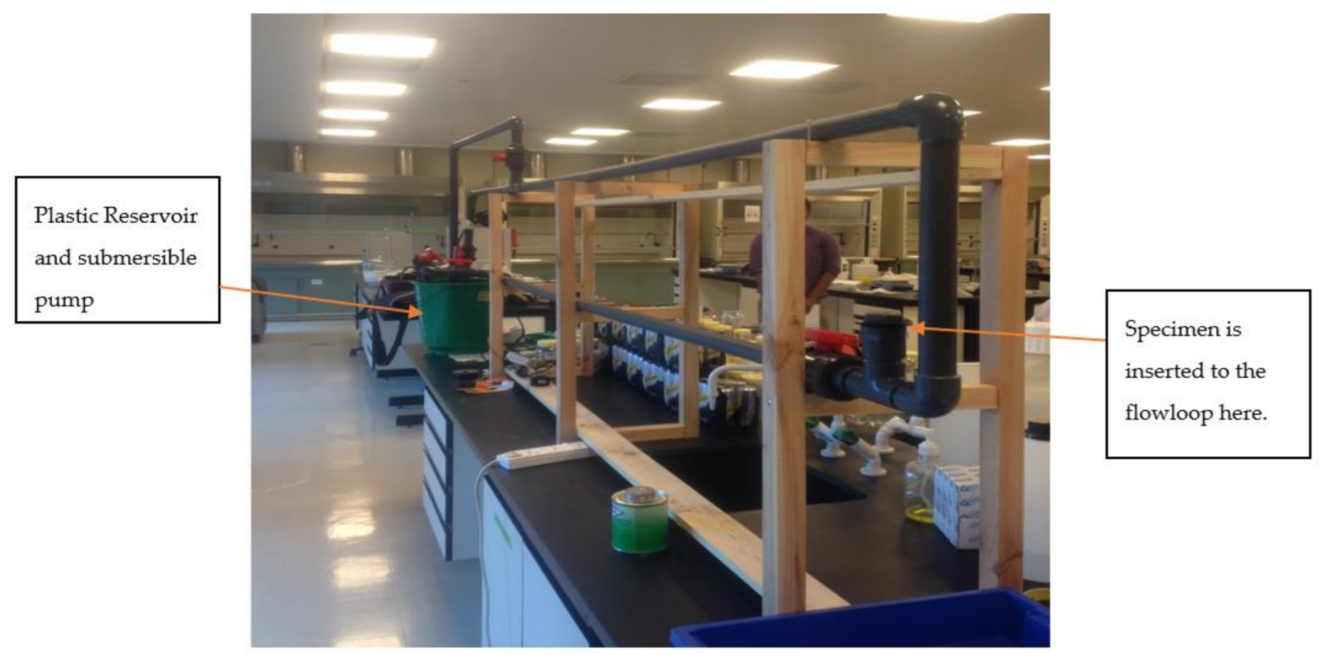
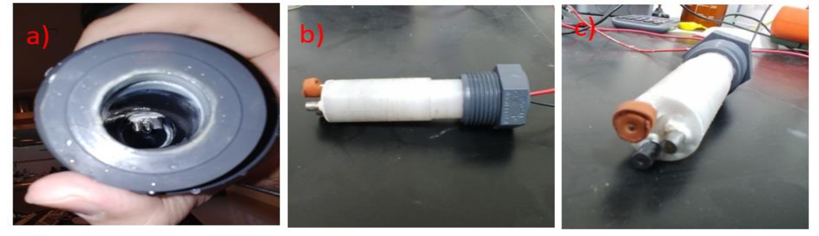
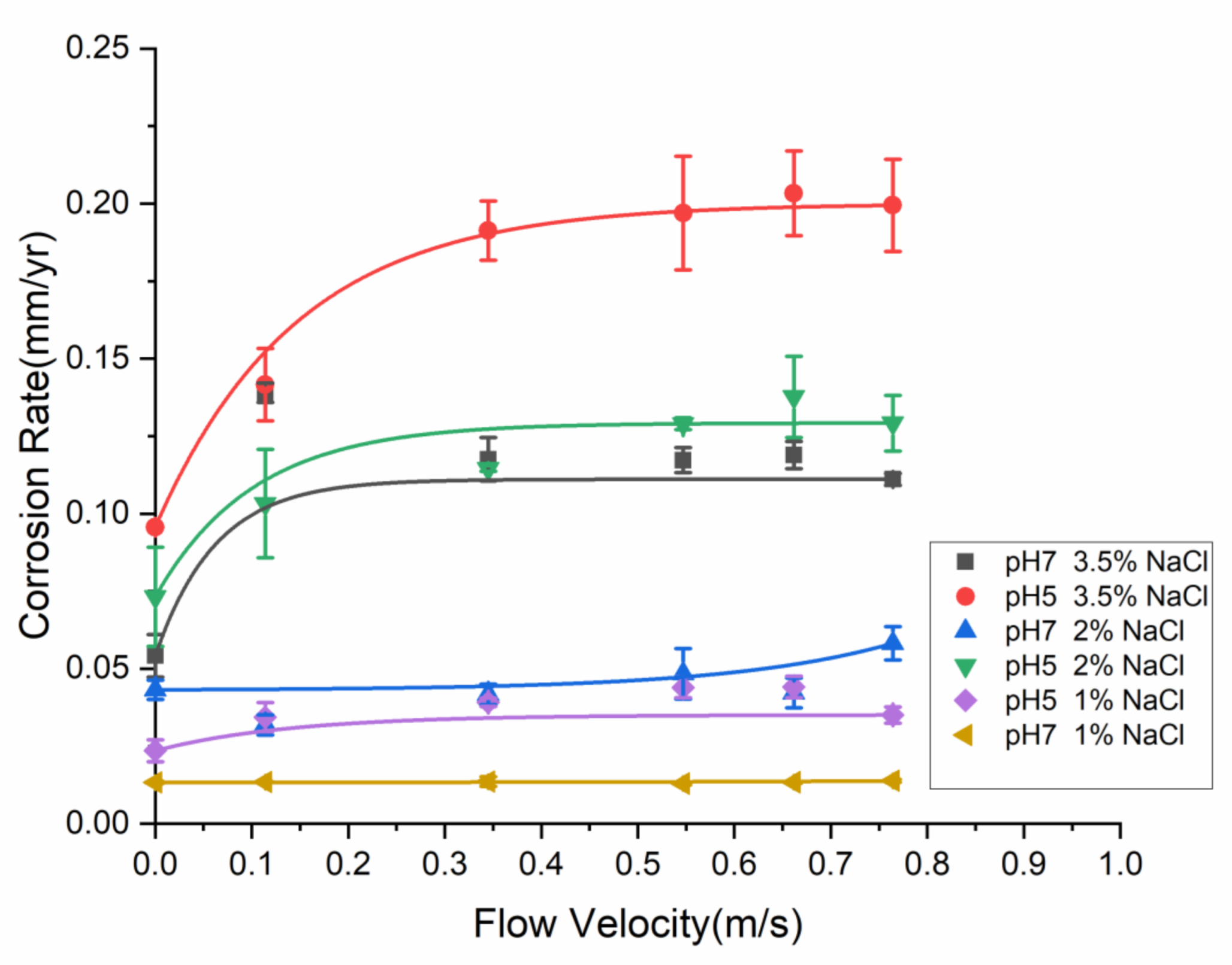
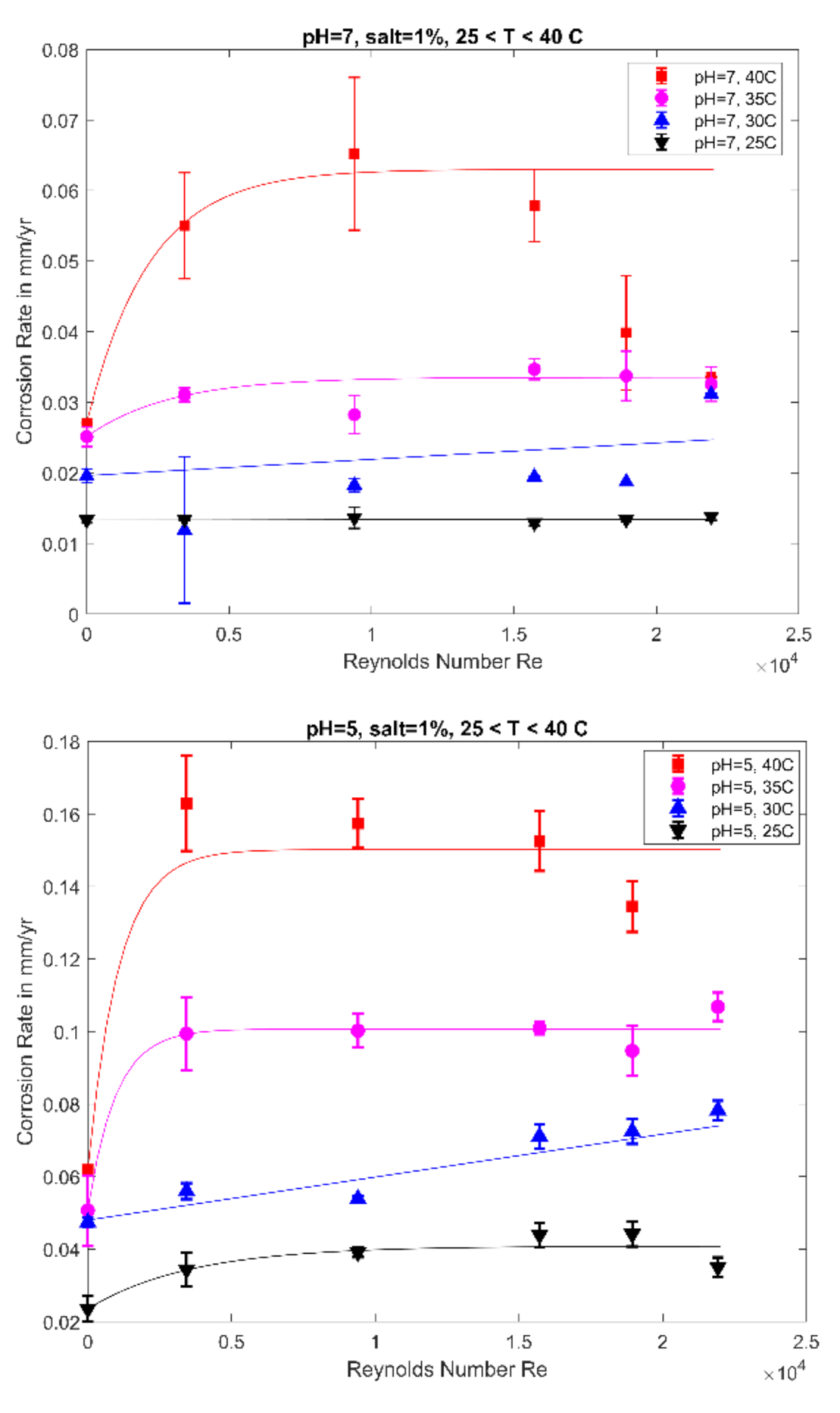
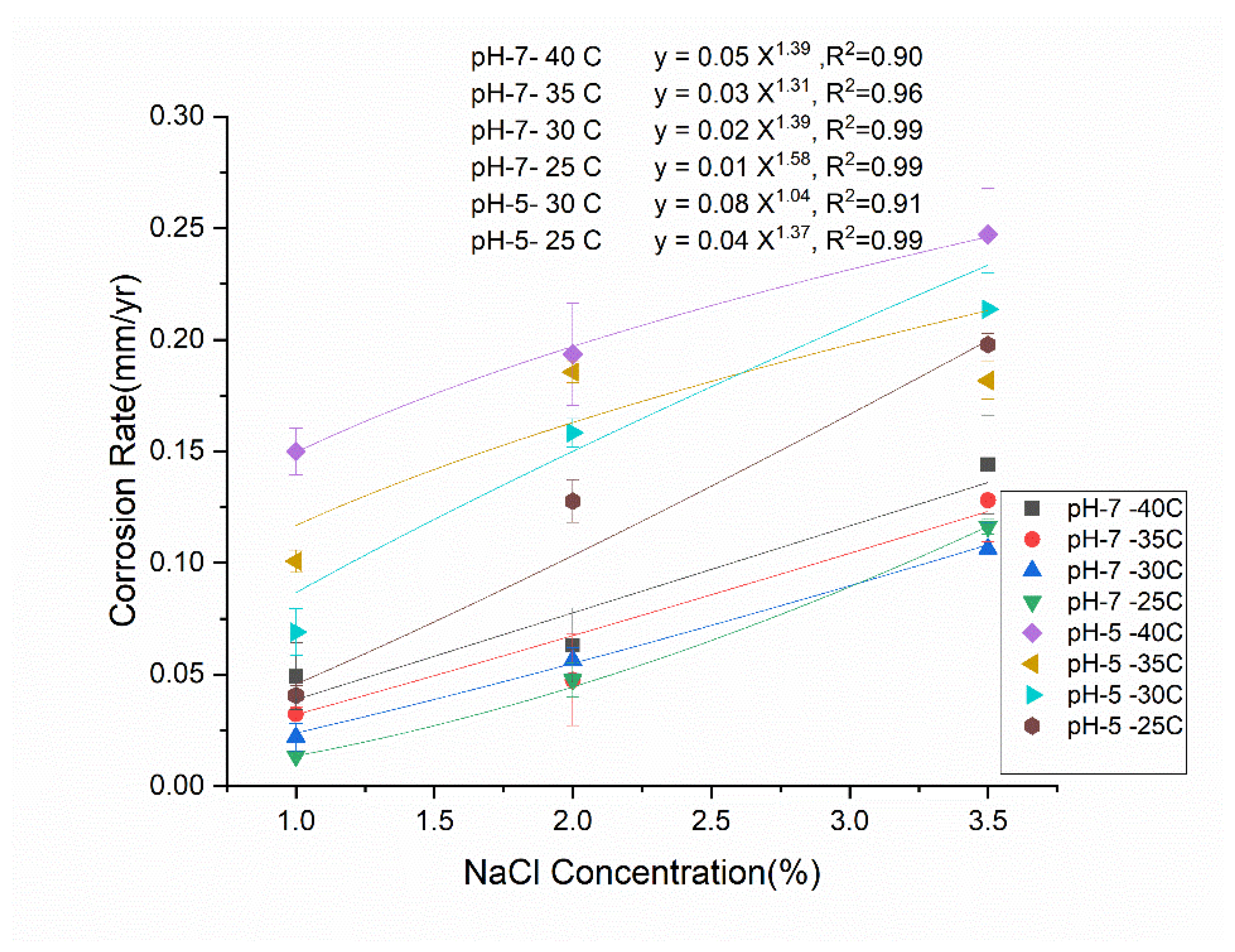
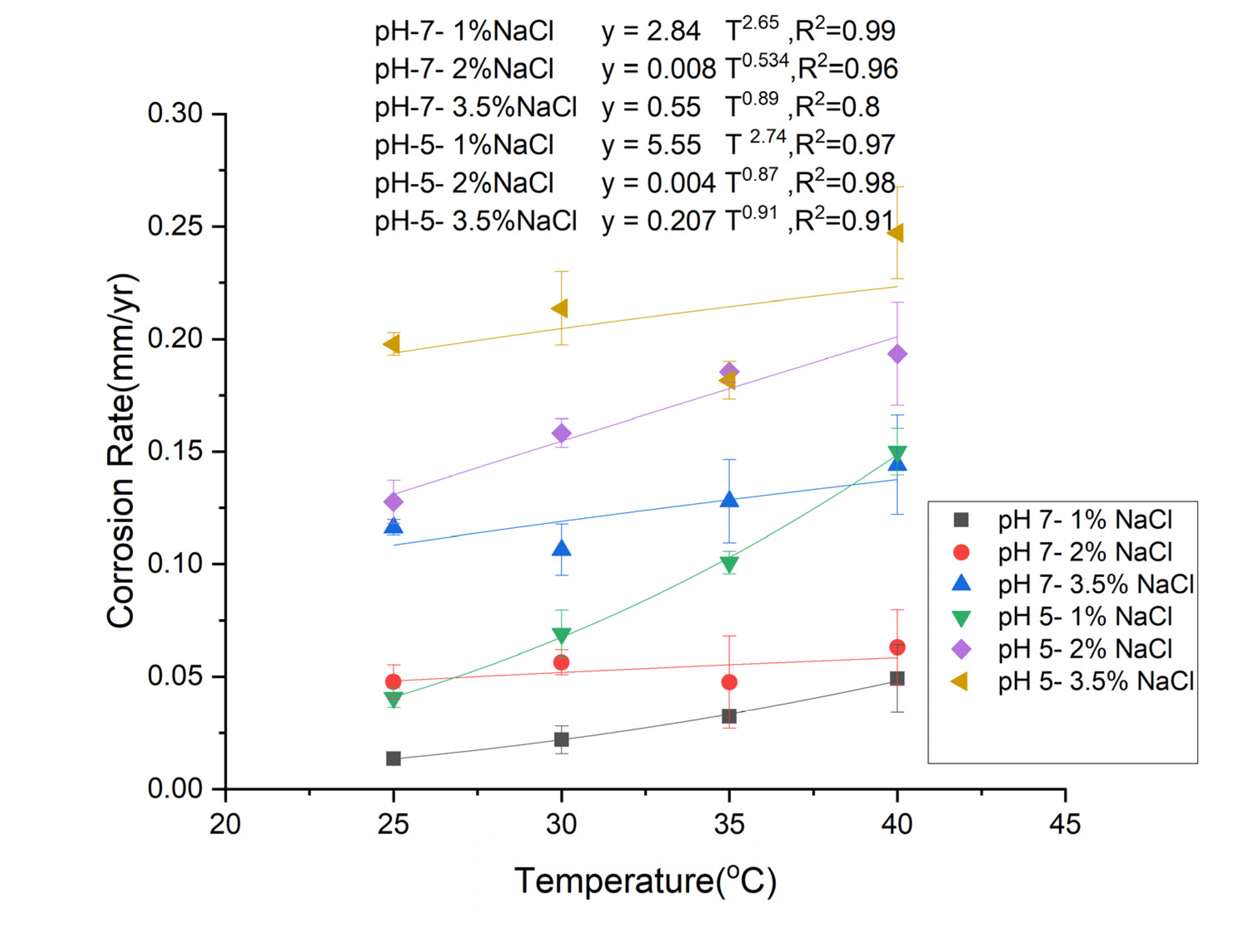
In this paper, corrosion studies of the pipeline carbon steel (API-5L-X65 QT steel) are done in a flow loop using the LPR method to investigate the parameters which will affect the corrosion rates. Parametric studies have been conducted by changing flow rate, NaCl concentration, temperature, and pH, while bubbling oxygen into the solution. Key to this work, however, was the rigorous control of all parameters save one. This parameter was varied, and the corrosion rate was determined as a function of flow velocity, which was continuously varied from 0 to 0.8 m/s. Upstream pipelines in oil industries exhibit flow fluctuations, and the material degradation will be maximum because of corrosion and erosion. This work focuses on identifying the flow regions where the uniform corrosion is dominating and to predict a range of flow velocities where the corrosion rates can be kept constant. In that flow regions, parametric studies are conducted to develop a correlation with flow conditions and other parameters aiming to develop a predictive equation to obtain corrosion rates. In this research, we intend to measure the corrosion rate in a pipeline system using tight control of parameters. This is necessary, since corrosion rates are affected by so many different parameters, some of which have exponential effects.

2. Materials and Methods

2.1. Experimental Test Set-Up

The test solutions are prepared from deionized water (1 × 10⁴ Ohm-cm⁻¹) produced from a Metrohm Ion exchange still, with pH 5.8 supplied from a 20L reservoir. Solutions are then made according to the required parameters. The concentration of NaCl in the test solution is varied from 1% to 3.5%. The pH of the test solution is maintained to the desired values using acetic acid sodium acetate buffer solutions. The pH of the test solution is measured using an Orion pH meter and monitored at infrequent intervals. The Orion pH meter is manually calibrated before each use. The dissolved oxygen content in the solution, which is a vital factor in the corrosion rate, is maintained by bubbling air into the reservoir at 6 mg/L (6ppm) and measured using a Milwaulkie D.O meter every hour. The corrosion electrode sensor is a 3-electrode sensor where the material sample is the working electrode, a graphite electrode is the counter electrode, and Ag/AgCl is the standard reference electrode. The three-electrode sensor is designed to fit into the flow and arranged such that the working electrode faces the oncoming flow. Microbial corrosion is prevented by the periodic addition (each day) of disinfectant (Dettol) to the solution.

A circulating loop system, as shown in Figure 2, was used for measuring the corrosion rate. The schematic diagram of the flow loop and the actual flow loop are shown in Figure 3 and Figure 4. The flow loop consists of a plastic reservoir, a 0.50 horsepower/0.37 kW submersible pump (made of plastic) with a float switch, a pipe (made of PVC plastic) of internal diameter 28.9 mm and an outer diameter of 33.55 mm, PVC pipe fittings, PVC valves, a plastic calibrated flow meter, and the electrode test section. A 20 L test solution is supplied from the reservoir using the submersible pump, and the flow velocity is changed and continuously monitored using the flow meter. The entire flow loop is purposely made from plastic to make sure the only corroding component in the flow loop is the test specimen. The operating conditions are maintained in desired values, and the temperature of the test solution is varied from 25 °C to 40 °C (±0.5 °C) in the study and the operating conditions are maintained at desired values. The temperature is maintained using a heating and cooling system and continuously measured using a thermocouple and a mercury thermometer at infrequent intervals. The corrosion electrode system is connected to Gamry 600 potentiostat and a computer with Gamry instruments software. After mounting the electrode system in the flow loop, the required flow rate is obtained by adjusting the manifold valves in the loop and varying the amount of bypass, and monitoring the LPM values in the digital gauge. Once the flow is stable, the potentiostat is turned on, the readings can be recorded, and further analysis can be performed using the respective Gamry software. After recording one reading, the sample is removed and cleaned before continuing the experiments. There is a 2.02 m run of straight unaffected pipe, equivalent to 69 diameters, to allow for a fully developed flow to occur and for pump noise to dissipate. The test specimen is at the bottom of a vertical flow loop, as shown in Figure 4. This is to ensure that only single-phase flow impinges on the test specimen. On the top (return) side of the loop, there is an additional deaerator that catches bubbles and ensures that, after a few minutes of flushing, the loop has no trapped bubbles in it and is a single phase.

2.2. Pipeline Steel

The working electrode was a 0.5 cm diameter API-5L-X65 QT (Quenched and Tempered) material. The microstructure of the steel is shown in Figure 5a,b from the optical micrograph of the samples consisting of ferrite and pearlite. The volume fractions of ferrite and pearlite have been measured to be ~77% and ~23%, respectively. The average ferrite to pearlite ratio is around 80% to 20%, as evident from the figure. The average grain size has been found to be ~15 μm. Figure 5c shows the SEM photograph of the mild steel sample after polishing. Like the optical micrograph, the grain distribution of the samples is clearly visible in the SEM images. The microstructure shows the carbon content is very low.

Three electrode (Specimen, Graphite, Ag/AgCl ) setup was constructed using a nylon support material (shown in white color) and the electrodes fixed in place using marine grade epoxy (PC 10—marine) to prevent movement and crevice corrosion, as shown in Figure 6. The electrode, covered by an orange cap, is the Ag/AgCl electrode, the dark gray electrode is the graphite, and the light gray electrode, is the API-5L-X65 QT specimen. The electrodes were designed to sit in the full flow of the system.

2.3. Linear Polarization Resistance

In this model, the corrosion process is assumed to be controlled by the kinetics of electron transfer reaction at the metal surface, and the electrochemical reaction can be expressed using the Tafel equation,

$$I=I_o{e}^{\frac{2.303\left(E-E_o\right)}{\beta }}$$

(1)

where I is the current resulting from the reaction, I_o is a reaction-dependent constant called the exchange current, E is the electrode potential, E_o is the equilibrium potential, and β is the Tafel constant (volts/decade).

The Tafel equation is generally used to express the behavior of one reaction, and it is modified to Butler-Volmer equation, which can express both anodic and cathodic reactions, and it is given by,

$$I=I_{corr}{e}^{\frac{-2.303\left(E-E_{corr}\right)}{{\beta }_a}} e^{\frac{-2.303\left(E-E_{corr}\right)}{{\beta }_c}}$$

(2)

where I is the current (amperes), I_corr is the corrosion current, E is the electrode potential, E_corr is the corrosion potential, and β_a and β_c are the anodic and cathodic Tafel constants in volts/decade.

From the Tafel analysis shown, the current-voltage curve at E_corr can be considered as linear, and Equation (2) can be modified to obtain the Stern-Geary equation.

$$I_{corr}=\frac{1}{R_P}\times \frac{{\beta }_a{\beta }_c}{2.303\left({\beta }_a+{\beta }_c\right)}$$

(3)

The corrosion current can be related to the corrosion rate using Faraday’s law,

$$Q=n\times F\times M$$

(4)

where Q is the charge in coulombs, n is the no of electrons transferred, F is Faraday’s constant (96,485 coulombs/mole), and M is the number of moles equal to M = m/AW, where AW is the atomic weight. Substituting the equivalent weight in terms of M in Equation (4), the mass of the species m can be written as,

$$m=\frac{\left(EW\right)Q}{F}$$

(5)

where EW is the equivalent weight. Modifying Equation (5) and substituting the value of Faraday’s constant, the corrosion rate (CR) is found to be:

$$CR=\frac{I_{corr}\times K\times EW}{d\left(A\right)}$$

(6)

where d is the density (g/cm³), A is the sample area in cm², and K is a constant.

Electrochemical measurements are performed using Gamry Reference 600 potentiostat. The experiments were conducted till the system reached the open circuit potential (OCP) before linear polarization resistance was measured. Figure 7 shows the OCP measurement where potential is plotted against time for 1%, 2%, and 3.5% NaCl concentrations at 25 °C when the flow velocity is kept at zero. OCP, also called corrosion potential, is the Potential difference between the working and reference electrode when no external current is flowing in the cell. OCP measurement allows us to determine the E_corr and gives a broad view of the stability of the system. The plot shows the OCP value becomes stable after 3600 s for three concentrations, and the test time for the experiments are kept at 1 h throughout the study. The area of the cylindrical electrode is 1.6cm² with a density of 7.87 g/cm³, the potential was swept between −0.02 Volts to 0.02 volts with a scan rate of 0.2 mV/s. The sample period was kept as 2 s, and Tafel analysis is conducted to determine the Tafel constants by running a potentiodynamic scan from −250 mV to 250 mV.

3. Discussion of Results

3.1. Experimental Observations and Analysis

Prediction of corrosion rate in the flow loop is a challenging task as various parameters affect the rates depending upon the material properties. The dissolved oxygen in the system is an important factor that controls the corrosion rate, since the corrosion mechanism is different whether the system is aerated or deaerated. The temperature of the fluid in contact, the flow rate of the fluid, the concentration of the chloride ions, dissolved salts, and pH are parameters that can enhance and reduce the corrosion rate of the mild steel in a flow system.

In this study, we investigated the effects of flow rate, temperature, pH, and NaCl concentration on corrosion rate by changing one of the parameters and keeping the other parameters constant. The study is conducted in two different pH levels, namely, pH-7 and pH-5. The pH is maintained by adding sodium acetate buffer solution and is monitored using a well-calibrated pH meter. The temperature of the feed solution is changed from 25–40 °C every 5 °C degrees, the flow rate of the solution in the loop is varied from 0–0.8 m/s (Reynolds number up to 22,000), and the salt concentration of the solution is varied from 1% to 3.5% by adding NaCl. The effect of velocity on corrosion rate has been studied previously, and the application of these findings in practical flow systems is very difficult. The corrosion rate and its relationship with flow velocity varies differently for different metals and alloys; thus, it is very challenging to form a specific conclusion. The changes in velocity alter the oxygen supply to the material and remove corrosion products from the specimen surface, thus resulting in different corrosion rates. Generally, at low flow rates, the corrosion rate will be uniform at the surface, and at higher flow rates, corrosion will be more localized, resulting from the formation of oxygen concentration cells. At higher flow rates, corrosion rates can sometimes increase because of increased oxygen supply and can decrease due to the destruction of thermal and concentration gradients. Here are the corrosion rate results, obtained from the flow loop of Figure 4.

Figure 8 presents the corrosion rate of API-5L-X65 steel in millimeter per year (1 mm = 0.0393 inches = 39.3 mils) versus flow velocity (between 0 and 0.8 m/s), as NaCl concentration varies from 1% to 3.5%, and temperature varies from 25 °C, 30 °C, 35 °C to 40 °C with the feed solution maintained at pH-7. The change in corrosion rate with the parameters, such as flow velocity, temperature, and NaCl concentrations is discussed in the figure. For flow velocities up to 0.2 m/s, the corrosion rate increases as the oxygen supply to the material increases, and at higher flow velocities (0.2 to 0.8 m/s), the corrosion rate appears to reach a steady value. It is assumed a stable oxide film is formed on the material surface, which provides a constant corrosion rate. At zero velocity, the corrosion rate is significant and shows an increasing trend with an increase in NaCl concentration and temperature. The formation of the black iron oxide layer is also observed on the metal surface when there is no flow. It can be observed from Figure 8, that at pH-7, the corrosion rate varies from 0.0254 mm/yr to about 0.2032 mm/yr when the NaCl concentrations vary from 1% to 3.5%. At a temperature of 25 °C, the corrosion rate is less than 0.0254 mm/yr for 1% NaCl concentration and the corrosion rates reach 0.0508 mm/yr and 0.1143 mm/yr at 2% and 3.5% NaCl, respectively. A corrosion rate of 0.0558 mm/yr is observed for 2% NaCl solution at 30 °C, and 0.0635 mm/yr at 35 °C. At 40 °C, the corrosion rates increase from 0.0508 mm/yr to 0.08636 mm/yr when NaCl concentration changes from 1% to 2%. Corrosion rate further increases and reaches a value of 0.1727 mm/yr is at 3.5% NaCl concentration.

The effect of flow velocities on the corrosion rates of API-5L-X65 QT is shown at different temperatures in Figure 9. When the feed solution is maintained at 1% NaCl concentration shown with black color lines (see Figure 9), the corrosion rate reaches 0.0782 mm/yr at 30 °C, 0.1028 mm/yr at 35 °C, and 0.1424 mm/yr at 40 °C. An increase in NaCl concentration to 2%, shown with blue color lines, causes an increase in the corrosion rates in the range of 0.1143 mm/yr to 0.2032 mm/yr when flow velocity and the temperature is varied. The red line shows corrosion rats at 3.5% NaCl concentration, and the corrosion rates are increased up to 15–28% than the 2% NaCl concentration conditions. At 40 °C, the corrosion rate reaches a maximum value of about 0.254 mm/yr (10mpy) at a flow velocity of 0.4 m/s, and a further increase in flow velocity is not affecting the corrosion rates. The increase in temperature shows a 5% to 10% increase in corrosion rates in all concentrations except for some data points.

In Figure 10, a study is conducted to determine the influence of pH on the corrosion rate. The results are shown at a temperature of 25 °C at different flow rates and NaCl concentration. In the literature, significant studies have been done that analyze the relation between pH and the corrosion rates, but very limited studies to model the effects in a flow loop, as discussed earlier. The physical and chemical properties of the corrosion products and the corrosion layer formed on the surface lead to variation in corrosion rates in different pH and flow velocities [28]. The studies show conflicting results at different pH as the high testing period leads to different corrosion mechanisms depending upon the material property [28]. As the LPR technique is short term method, observed trends eliminate the possibilities of different corrosion mechanisms at different pH and show a consistent trend in corrosion rates. At zero velocity for pH 7, the corrosion rate observed is about 0.04321 mm/yr for 2% concentrated solution and 0.05419 mm/yr for 3.5% NaCl solution. When the pH is maintained at 5, at zero velocity, the corrosion rate observed is 0.0732 mm/yr for 2% NaCl solution, and at 3.5% NaCl concentration, the corrosion rate shows an increase of 75% than pH 7 and records a value of 0.0956 mm/yr. As shown in the previous results (Figure 8 and Figure 9) at different pH and temperatures, the majority of the data suggests that the corrosion rate is insensitive to flow at high velocities and maintains a steady rate. The results of Figure 8 and Figure 9 show the corrosion rate tends to increase when the hydrogen ion concentration in the feed solution increases.

3.2. Parametric Study in Flow Insensitive Region

The results discussed in the previous section consistently shows two different regimes. A flow-sensitive region, where small changes to the flow or Reynolds number (Re) results in an exponential increase in corrosion rate and a flow insensitive region where the increase in flow rate does not affect the corrosion rate of the sample. This constant rate corrosion flow region is visible in most graphs, but not all.

Figure 11 shows the flow insensitive region, the corrosion rates are shown at different Reynolds number for 1% NaCl concentration for pH of 7 and 5 at different temperatures. In all the cases shown in Figure 11, the flow insensitive region is visible, corrosion rates are increasing with Reynolds number, and when Re is above 5000, the corrosion rates reach a plateau. It is assumed that a corrosive oxide layer formed on the surface limits the flow to the metal surface, and it minimizes the diffusion of hydroxides from the steel surface to the flowing water, which reduces the ion concentrations in the interfaces. The corrosion rate in the corrosion insensitive flow region is where uniform corrosion is predominant, and that region can be utilized to derive correlations for corrosion behavior at different operating parameters. The identification and analysis of this flow insensitive region in pipelines will be valuable in corrosion prediction and control.

The corrosion rates in the flow-insensitive region are taken as constant when the Reynolds number are greater than 10,000, and the corrosion rates are plotted with temperature, salinity, and pH to find the correlation between the parameters. pH and NaCl concentrations have a significant effect on corrosion rate like temperature, and the relationship is derived using the corrosion rates obtained in the flow insensitive region. The analysis, shown in Figure 12, provides the relation between NaCl concentration and corrosion rates. The corrosion rate, influenced by the presence of chloride ion, can cause the acceleration of both the anodic and cathodic reactions. The plot is analyzed, and the corrosion rate seems to increase as the power of NaCl concentration (X = NaCl concentration) and from the figure, the experimental data shows a good match with the power equation. It can be seen from Figure 12 that there is a good fit between the experimental data and the power equation with the coefficient of determination (R²) above 0.9. To create one equation that can define the corrosion rate as a function of NaCl concentration (X), an average constant exponent value around 1.4 was chosen. The corrosion rates can be expressed as $A{x}^{1.4}$ and a constant, which depends on the other flow parameters. Thus, the following relations CR = A (NaCl Concentration)^1.4 can be obtained to correlate the corrosion rates with NaCl concentration.

The corrosion rates from the flow insensitive region are plotted against the temperature, and the corrosion rates at pH 7 and 5 are plotted for 1%, 2%, and 3.5% NaCl solution. The corrosion rate in the mild steel samples seems to increase with the temperature in the flow insensitive region. At pH 7 for 2% NaCl concentrations, the corrosion rates increase from 0.0484 mm/yr to 0.0660 mm/yr when the temperature increases from 25 ° to 40 °C, whereas for the 3.5% NaCl concentration the corrosion rate changes from 0.1143 mm/yr to 0.1524 mm/yr. The data in the flow insensitive region is analyzed to predict the corrosion change with temperature. The exponential relationship between corrosion rates and temperature given by Arrhenius is widely used in the corrosion prediction. Arrhenius gave the equation in static conditions as K = A exp(-E_a/RT), where K = rate constant, R = gas constant (8.314 J\mole), T = temperature in degree Kelvin, E_a = activation energy (J\mole.K), and A = Modified frequency factor (pre-exponential factor). An attempt was made to fit the Arrhenius equation to the experimental data, but the fit was not good. The analysis, shown in Figure 13, reveals that the corrosion rate can be expressed as a power equation of temperature, showing a much better fit than the Arrhenius equation. In all the cases studied, the power constant varies when the NaCl concentration changes from low (1%) to high (3.5%). For both pH 5 and 7 at 1%NaCl concentration, the power constant is found to be about 2.7, but when the NaCl concentration is increased to 3.5%, the power constant is found to be about 0.9. The corrosion rates can be expressed as AT^0.9 for high NaCl concentration. Therefore, the following relation between the corrosion rate and the temperature is proposed: Corrosion Rate = A (Temperature)^0.9 for high salinity. The value of the coefficient A was found to be varying with both NaCl concentration and pH. The correlation for temperature concludes that more data points need to be obtained in order to be able to generalize an empirical formula.

The parametric study was conducted by maintaining constant oxygen concentration in the system. The oxygen concentration affects the corrosion rate of mild steel in NaCl, and the solubility of the oxygen will be an important factor in the predictive equation. In the work presented in this paper, individual equations (as shown in Figure 12 and Figure 13) relating the corrosion rate in low flow velocities are developed. In future studies, the work will look at the synergistic effects of changing two or more parameters at the same time at different oxygen concentrations. This eventually leads towards a predictive model of the corrosion in pipelines and identifying the flow regions where corrosion rates can be minimized.

4. Conclusions

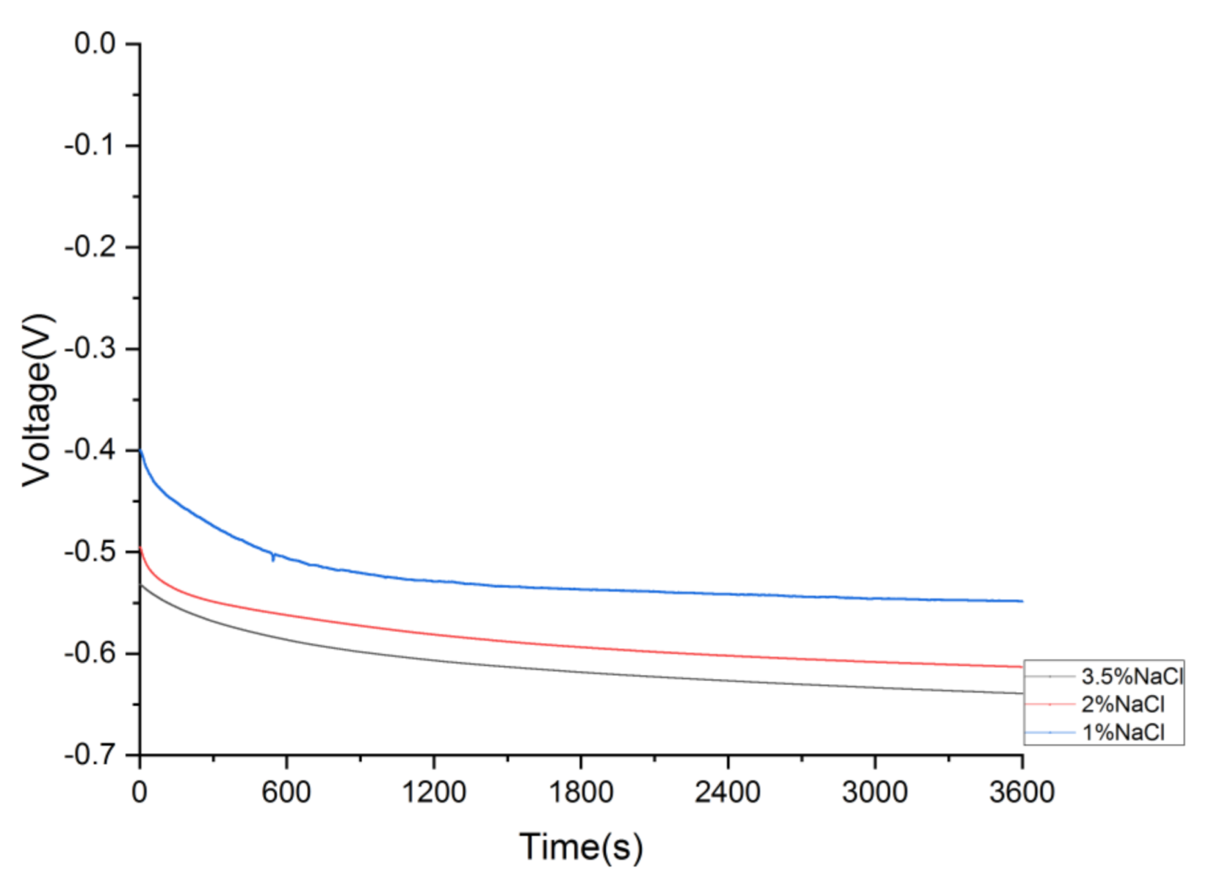
Using the linear polarization resistance (LPR) method and the work presented in this paper, we have been able to make repetitive measurements of the corrosion rate of API-5L-X65 QT steel—taking an average of at least three measurements per parameter. For each test condition, one parameter was varied, while all other parameters were kept constant. This level of detail is essential to assess the true effect of each parameter on the corrosion rate.

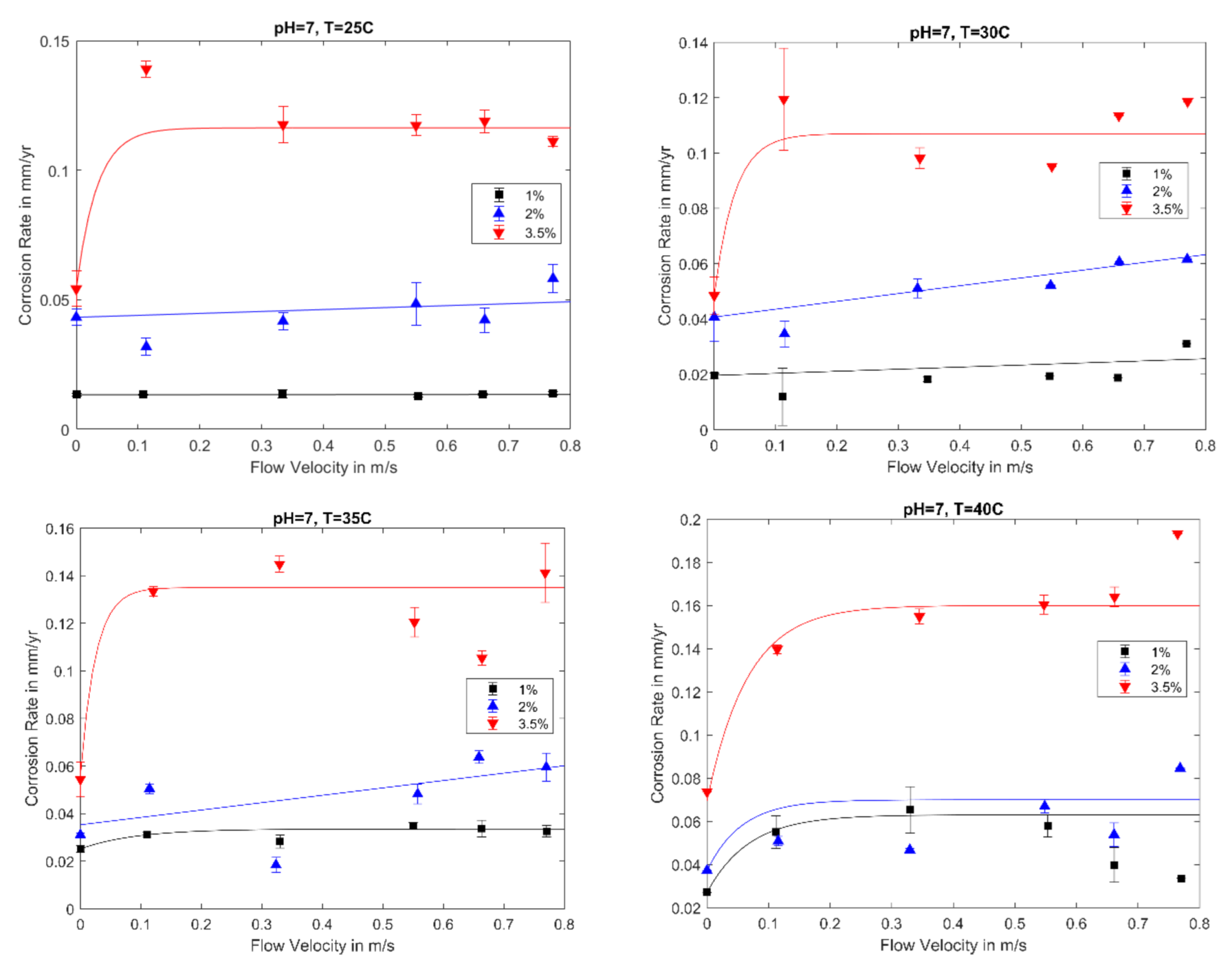
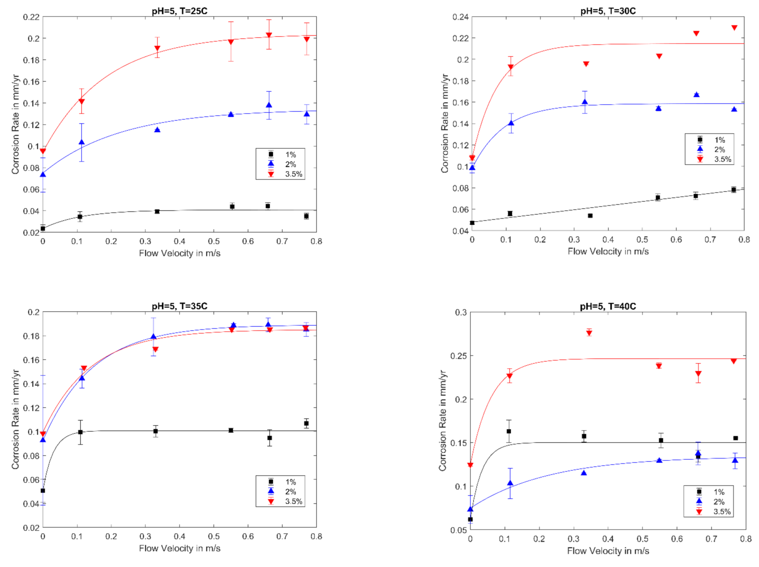
Experimental data presented in this work indicates a complex relationship between pH level, temperature, salt concentration, flow velocity, and corrosion rate. For the majority of combinations of experimental parameters, one can observe a range of flow velocities where the corrosion rate reaches a quasi-steady state or exhibits a linear behavior. The complex behavior where the corrosion rate is best described by exponential functions is mostly observed for cases with pH = 5. For pH = 5, the exponential function, that fits the experimental data very well, has the form $c_r=a+b{e}^{-cv}$ where c_r is the corrosion rate, v is the fluid velocity, and a, b, and c are the fitting constants. The majority of the experimental data, but not all, suggests that in the velocity range of 0.2 m/s to 0.8 m/s, the corrosion mechanism appears to be uniform corrosion, and erosion corrosion is not occurring. Near fluid velocity of 0.8 m/s, an increase in corrosion rate is observed in most cases but not all. Turbulence-induced erosion corrosion maybe occurring. The highest corrosion rate occurs at 40 °C and 3.5% salt concentration, and the corrosion rate is about 0.25 to 0.3 mm/yr.

In this paper, we have also produced individual equations relating to the corrosion rate to a given parameter. In the future, it is our intention to look at the synergistic effects of changing two or more parameters at the same time and study their effects on the corrosion rate of oil pipelines. Eventually, this work will lead towards a predictive model of the corrosion rate in mild steel pipelines. Since API-5L-X65 material is widely used in the oil industry, the experimental data collected and published in this paper can be very useful to corrosion engineers working in the oil industry.

References

1. Koch, G. Cost of Corrosion; Woodhead Publishing Series in Energy: Cambridge, UK, 2017; pp. 3–30. [Google Scholar]
2. Shekari, E.; Khan, F.; Ahmed, S. Economic risk analysis of pitting corrosion in process facilities. Int. J. Press. Vessel. Pip. 2017, 157, 51–62. [Google Scholar] [CrossRef]
3. El-Sherik, A. Trends in Oil and Gas Corrosion Research and Technologies: Production and Transmission; Woodhead Publishing: Cambridge, UK, 2017. [Google Scholar]
4. Liu, J.; BaKeDaShi, W.; Li, Z.; Xu, Y.; Ji, W.; Zhang, C.; Cui, G.; Zhang, R. Effect of flow velocity on erosion–corrosion of 90-degree horizontal elbow. Wear 2017, 376, 516–525. [Google Scholar] [CrossRef]
5. Rostron, P. Critical review of pipeline scale measurement technologies. Indian J. Sci. Technol. 2018, 11. [Google Scholar] [CrossRef]
6. Copson, H. Effects of velocity on corrosion. Corrosion 1960, 16, 86t–92t. [Google Scholar] [CrossRef]
7. Namboodhiri, T.; Upadhyay, S. Flow-assisted corrosion of API X-52 steel in 3.5% NaCl solution. Can. J. Chem. Eng. 2002, 80, 456–464. [Google Scholar]
8. Zhang, G.; Zeng, L.; Huang, H.L.; Guo, X.P. A study of flow accelerated corrosion at elbow of carbon steel pipeline by array electrode and computational fluid dynamics simulation. Corros. Sci. 2013, 77, 334–341. [Google Scholar] [CrossRef]
9. Utanohara, Y.; Murase, M. Influence of flow velocity and temperature on flow accelerated corrosion rate at an elbow pipe. Nucl. Eng. Des. 2019, 342, 20–28. [Google Scholar] [CrossRef]
10. Compton, R.G.; Sanders, G.H. Electrode Potentials; Oxford University Press Oxford: Oxford, UK, 1996. [Google Scholar]
11. Zafar, M.N.; Rihan, R.; Al-Hadhrami, L. Evaluation of the corrosion resistance of SA-543 and X65 steels in emulsions containing H2S and CO2 using a novel emulsion flow loop. Corros. Sci. 2015, 94, 275–287. [Google Scholar] [CrossRef]
12. Ajmal, T.; Arya, S.B.; Udupa, K.R. Effect of hydrodynamics on the flow accelerated corrosion (FAC) and electrochemical impedance behavior of line pipe steel for petroleum industry. Int. J. Press. Vessel. Pip. 2019, 174, 42–53. [Google Scholar] [CrossRef]
13. Huang, H.; Tian, J.; Zhang, G.; Pan, Z. The corrosion of X52 steel at an elbow of loop system based on array electrode technology. Mater. Chem. Phys. 2016, 181, 312–320. [Google Scholar] [CrossRef]
14. Sun, Y.; Nesic, S. A parametric study and modeling on localized CO2 corrosion in horizontal wet gas flow. In Corrosion 2004; NACE-04380; Nace International: New Orleans, LA, USA, 2004. [Google Scholar]
15. De Waard, C.; Milliams, D. Carbonic acid corrosion of steel. Corrosion 1975, 31, 177–181. [Google Scholar] [CrossRef]
16. De Waard, C.; Lotz, U.; Milliams, D. Predictive model for CO2 corrosion engineering in wet natural gas pipelines. Corrosion 1991, 47, 976–985. [Google Scholar] [CrossRef]
17. Jepson, W.P.; Bhongale, S.P.; Gopal, M.P. Predictive model for sweet corrosion in horizontal multiphase slug flow. In Corrosion 1996; NACE-96019; Nace International: Denver, CO, USA, 1996. [Google Scholar]
18. Nesic, S.; Cai, J.; Lee, K.-L. A multiphase flow and internal corrosion prediction model for mild steel pipelines. In Corrosion 2005; NACE-05556; Nace International: Houston, TX, USA, 2005. [Google Scholar]
19. Pots, B.F. Prediction of corrosion rates of the main corrosion mechanisms in upstream applications. In Corrosion 2005; NACE-05550; NACE International: Houston, TX, USA, 2005. [Google Scholar]
20. Khajotia, B.; Sormaz, D.; Nesic, S. Case-based reasoning model of CO2 corrosion based on field data. In Corrosion 2007; NACE-07553; Nace International: Nashville, TN, USA, 2007. [Google Scholar]
21. Olsen, S. CO2 corrosion prediction by use of the Norsok M-506 model-guidelines and limitations. In Corrosion 2003; NACE-03623; Nace International: San Diego, CA, USA, 2003. [Google Scholar]
22. Nyborg, R. CO2 Corrosion Models for Oil and Gas Production Systems. In Corrosion 2010; NACE-10371; Nace International: San Antonio, TX, USA, 2010. [Google Scholar]
23. Cabrera-Sierra, R.; Cosmes-López, L.J.; Castaneda-López, H.; Calderón, J.T.; López, J.H. Corrosion Studies of Carbon Steel Immersed in NACE Brine by Weight Loss, EIS and XRD Techniques. Int. J. Electrochem. Sci. 2016, 11, 10185–10198. [Google Scholar] [CrossRef]
24. Han, J.; Carey, J.W.; Zhang, J. Effect of sodium chloride on corrosion of mild steel in CO2-saturated brines. J. Appl. Electrochem. 2011, 41, 741–749. [Google Scholar] [CrossRef]
25. Nesic, S.; Wang, S.; Fang, H.; Sun, W.; Lee, J.K. A new updated model of CO2/H2S corrosion in multiphase flow. In Corrosion 2008; NACE-08535; Nace International: New Orleans, LA, USA, 2008. [Google Scholar]
26. Zeng, Z.; Lillard, R.; Cong, H. Effect of salt concentration on the corrosion behavior of carbon steel in CO2 environment. Corrosion 2016, 72, 805–823. [Google Scholar] [CrossRef]
27. Han, J.; Carey, W.; Zhang, J. A coupled electrochemical–geochemical model of corrosion for mild steel in high-pressure CO2–saline environments. Int. J. Greenh. Gas Control 2011, 5, 777–787. [Google Scholar] [CrossRef]
28. Scheers, P. The effects of flow velocity and pH on the corrosion rate of mild steel in a synthetic minewater. J. S. Afr. Inst. Min. Metall. 1992, 92, 275–281. [Google Scholar]
Figure 1. Different Corrosion models and predicted corrosion rates (Field data from [22] for the oil well 5.).
Applsci 11 00444 g001
Figure 2. Flow loop for investigating corrosion using LPR method.
Applsci 11 00444 g002
Figure 3. A layout of the experimental setup.
Applsci 11 00444 g003
Figure 4. The actual flow loop.
Applsci 11 00444 g004
Figure 5. The microstructure of the steel is studied using optical microscopic images of the metal sample and shown (a) 20-micrometer (b) 100-micrometer (c) SEM images of the surface.
Applsci 11 00444 g005
Figure 6. (a) Projection of sensor electrodes into the flow (b) isometric view of the sensor (c) side view. The orange rubber cap keeps the reference sensor (Ag/AgCl) from drying out.
Applsci 11 00444 g006
Figure 7. Potential is plotted against time for 1%, 2%, and 3.5% NaCl concentrations at 25 °C when the flow velocity is kept at zero.
Applsci 11 00444 g007
Figure 8. Corrosion rates of API-5L-X65 QT are shown at different flow velocities for feed solution maintained at pH-7, varying NaCl concentrations and temperatures (25 °C, 30 °C, 35 °C, and 40 °C).
Applsci 11 00444 g008
Figure 9. Corrosion rates of API-5L-X65 QT are shown at different flow velocities for feed solution maintained at pH-5 varying NaCl concentrations and temperatures (25 °C, 30 °C, 35 °C, and 40 °C).
Applsci 11 00444 g009
Figure 10. Corrosion rates of API-5L-X65 QT metal are shown at different flow velocities maintaining the feed solution pH of 5 and 7 and varying NaCl concentrations at 25 °C.
Applsci 11 00444 g010
Figure 11. Corrosion rates are shown at different Reynolds number for feed solution maintained at pH–7 on the left, and at pH-5 on the right at 1% NaCl, at following temperatures (25 °C, 30 °C, 35 °C, and 40 °C).
Applsci 11 00444 g011
Figure 12. Corrosion rates for flow insensitive region are fitted with varying NaCl Concentration.
Applsci 11 00444 g012
Figure 13. Corrosion rates at different temperatures for flow insensitive regions are fitted using Power-law.
Applsci 11 00444 g013
Publisher’s Note: MDPI stays neutral with regard to jurisdictional claims in published maps and institutional affiliations.