A Novel Evolution Strategy of Level Set Method for the Segmentation of Overlapping Cervical Cells

Abstract

Development of an accurate and automated algorithm to completely segment cervical cells in Pap images is still one of the most challenging tasks. The main reasons are the presence of overlapping cells and the lack of guiding mechanism for the convergence of ill-defined contours to the actual cytoplasm boundaries. In this paper, we propose a novel method to address these problems based on level set method (LSM). Firstly, we proposed a morphological scaling-based topology filter (MSTF) and derived a new mathematical toolbox about vector calculus for evolution of level set function (LSF). Secondly, we combine MSTF and the mathematical toolbox into a multifunctional filtering algorithm 2D codimension two-object level set method (DCTLSM) to split touching cells. The DCTLSM can morphologically scale up and down the contour while keeping part of the contour points fixed. Thirdly, we design a contour scanning strategy as the evolution method of LSF to segment overlapping cells. In this strategy, a cutting line can be detected by morphologically scaling the union LSF of the pairs of cells. Then, we used this cutting line to construct a velocity field with an effective guiding mechanism for attracting and repelling LSF. The performance of the proposed algorithm was evaluated quantitatively and qualitatively on the ISBI-2014 dataset. The experimental results demonstrated that the proposed method is capable of fully segmenting cervical cells with superior segmentation accuracy compared with recent peer works.

1. Introduction

Cervical cancer, which is primarily caused by the infection of some types of Human Papilloma Virus (HPV), is one of the most common gynecological cancer in the world and has a very high probability of fatality if it is left untreated [1,2,3]. However, if the precursor lesions caused by HPV can be detected, it is quite possible to cure cervical cancer. Fortunately, cervical tumor has a precancerous condition that can be recognized and treated early, so cervical cancer has a great potential for prevention and cure. Over the past three decades, cervical cancer incidence and mortality rates have decreased by more than 50%, and most of the reduction is attributed to the Papanicolaou (Pap) smear screening technique introduced by [4] for detecting the precursor lesions of cervical cancer [5]. However, it still leaves much to be desired.

The Pap smear screening work in current clinical practice is mainly performed manually by cytotechnologists who must be critically trained and well-experienced. This manual process is very difficult and time consuming, and cytotechnologists are susceptible to make erroneous decisions [6] mainly caused by intra- and interobserver variability. Therefore, as a preparatory work of automated diagnosis, automated slide analysis has been a research focus. As the most essential task in automated slide analysis, the automated segmentation of cervical cells in the extended depth-of-field (EDF) images captured in different fields of view (FOVs) [7] is an ongoing concern [8,9,10]. Although some work has been done for cervical cell segmentation, such as segmentation of isolated cells (i.e., free-lying cells) and nuclei, it is still a challenge to develop an accurate and complete segmentation algorithm for overlapping cells in Pap images [10]. Due to the influence of poor contrast, overlapping, folding, polymorphic nonconvex shapes and the impurity introduced from the cell deposition process, accurate and complete segmentation of cytoplasm from cellular clumps in Pap images is the biggest obstacle for this challenge. Therefore, it is essential to develop a new system that can commendably carry out automated segmentation of overlapping cytoplasm for cervical cells in the Pap images.

The literature reviews about related studies on segmentation of cervical cells are in the following. Prior to the first attempt [11] to segment the overlapping cervical cells completely, the systems could be divided into three groups, including (1) segmentation of the nuclei [12,13,14,15,16,17,18] of cells, (2) segmentation of the isolated cells [19,20,21] and (3) segmentation of clusters of cells crowded together (i.e., cellular clumps) [22]. Then, a few complete segmentation systems for overlapping cervical cells emerged in recent years. In general, the main algorithms used in these systems can be roughly classified into the following algorithm groups: (1) graph-based methods [22,23,24,25,26], (2) morphological processing-based methods [27,28,29] and (3) level set method (LSM)-based approaches [30,31,32,33]. Graph-based methods, such as Voronoi diagram method [23], provide a new idea for cervical cells segmentation; however, the segmentations look unnatural. Morphological processing-based methods are simply to be used but rely on the parameter configuration. The LSM-based approach is more suitable for completely automated cervical cell segmentations, because it is less dependent on seeds initialization and parameter configuration. As an effective method for object delineation, LSM was first proposed by [34]. In the development of LSM, scientists contributed some classic works. For instance, after the original snake model was proposed in [35], a geometrically flexible and topologically changeable snake model was introduced independently [36,37] by partial differential equation (PDE) and has been successfully applied in two- and three-dimensional spaces. After Mumford [38] first proposed a functional framework for image segmentation based on the variation method and Zhao [39] first introduced the Heaviside and Delta functions to represent the length and area of the region delineated by level set function (LSF), Chan [40] proposed a successful region-based LSM known as the C-V model. Moreover, based on the previous works [38,41], Chen [42] first proposed an edge-based LSM with a prior shape. Li [43] proposed a new LSM (DRLSE) without periodic reinitialization LSF as signed distance function (SDF). DRLSE is used in the baseline method [33] to speed up the contour evolution. LSM can be used to detect the textural edges like Canny edge detector [44], because its adaptive topology changes can fit multiple target contours at the same time. The LSM can even control non-closed curves in three-dimensional space by means of the codimension two-level set method (CTLSM), which was first carried out by [45] and developed by [46]. In addition, the LSM has been successfully applied in image segmentation tasks [25,47,48,49]. Lu [33] proposed an algorithm for cervical cells segmentation based on multiple level set functions, which has been regarded as the baseline and comparative algorithm by a lot of literature [26,28,50,51,52,53,54]. However, it has a problem that the poorly initialized level set function never converges to the cell boundaries.

With the rapid improvement of the graphic processing unit (GPU), CNNs (convolutional neural networks) have been widely used in the field of medical image segmentation. However, these methods mainly focus on clinical parameters, such as the volume and shape obtained from organ and structure segmentation for quantitative analysis and organ substructure obtained from lesion segmentation for histopathological diagnosis [55]. After the U-net was introduced by Ronneberger [56], U-net-like architecture convolutional neural networks have achieved good results in semantic segmentation tasks, such as the segmentations of organs, tissues or lesions areas in CT, X-ray and MR medical images. In contrast, cervical cell segmentation is more like an instance segmentation task that attempts to delineate all cells from Pap images to separated instances. Although CNN-based methodologies, such as Mask R-CNN [57], have good performances for instance segmentation, they are not suitable for the automated and complete cervical cells segmentation, because the overlapping regions in pairs of overlapping cells cannot be separated. In the latest proposed panoptic segmentation task, which combines semantic with instance segmentation, nonoverlapping is clearly declared in the seminal work [58]. Therefore, CNN-based segmentation methods are difficult to use to achieve end-to-end cervical cell segmentation. This means classical image processing strategies are essential for CNN-assisted methods [22,59] that are successfully used in the segmentation of overlapping cervical cells. Moreover, the other obstacle for cervical cell segmentation by CNNs is a lack of datasets, and the CNN-based segmentation methods are particularly dependent on datasets.

In this paper, we propose a novel method to automatically segment the cytoplasm of touching and overlapping cells in Pap images. Our proposed method is capable of fully segmenting cervical cells compared with the method that can only segment isolated cells or segment regions of cellular clumps [60,61]. Our method is unsupervised, which provides the possibility for cervical cell segmentation with limited data, and is potentially more valuable in guiding automated slide analysis for cervical pathology. The main goal of the proposed method is to alleviate nonconvergence of the level set function (LSF) in delineating the overlapping regions of cells caused by poor initialization of the cellular contours in [33].

Our main contributions lie in the following aspects:

(1)

We designed a morphological scaling-based topology filter (MSTF) to filter out the false positive fragments caused by improper allocation of the initial contour points of touching cells (i.e., misallocation). In MSTF, we constructed the signed distance function (SDF) as the LSF of the initialized cytoplasm contour based on the linear time Euclidean distance transform (LTEDT) algorithm [62], which is denoted by LTEDT-SDF.

(2)

We theoretically derived a new mathematical toolbox about vector calculus for evolution of the LSF as the supplementary for the codimension two-level set method (CTLSM) [63], aiming to keep the initialized contours of the nonoverlapping region fixed. Our proposed evolution method of partially fixed contour is called the 2D codimension two-object level set method (DCTLSM), which can alleviate the accuracy loss of a MSTF.

(3)

We proposed a novel evolution strategy of LSF inspired by the watershed method [64]. In this strategy, we provided an effective guidance mechanism for attracting and repelling the LSF to converge towards its actual cell boundary.

(4)

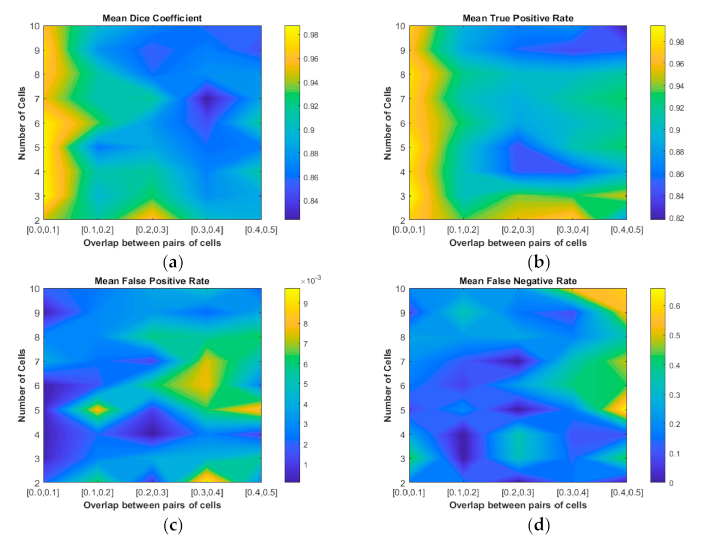
We used the dataset published by the First Overlapping Cervical Cytology Image Segmentation Challenge held in conjunction with the IEEE International Symposium on Biomedical Imaging (ISBI-2014 challenge) to evaluate our proposed method. The experimental results showed that cellular clumps consisting of two to 10 cells under an overlap ratio less than 0.2 can be accurately segmented. Furthermore, the segmentation of cellular clumps consisting of two to four cells can be effectively segmented with an overlap ratio less than 0.5. By qualitive and quantitative comparisons, our method outperformed the other segmentation methods.

2. Methodology

As shown in Figure 1, the architecture of the proposed method consists of contour initialization, touching cell splitting (pink arrow) and overlapping cell segmentation (purple arrow). In Section 2.1, the contour initialization includes nuclei detection and segmentation, as well as the segmentation of the contours formed by the boundary of the cellular clumps. After contour initialization, we obtained the initial contour of cytoplasm for each cervical cell. Based on this initialization, we proposed a new method for the touching cell splitting described in Section 2.2 and overlapping cell segmentation described in Section 2.3. As a major task, the proposed touching cell splitting (pink arrows) can alleviate the effect of misallocation of the pixels on the clump boundary, which may cause the cells slight touching or the isolated ones misjudged as overlapping. After the isolation judgement of the isolated cells, the algorithm proceeds to the overlapping cell segmentation, which is the other major task, aiming to segment the overlapping cell from its neighbor cells iteratively.

2.1. Cellular Component Segmentation

The goal of cellular component segmentation is to achieve contour initialization by nuclei detection and cellular clump segmentation. In this paper, we used the contour initialization method [33], because it provides an efficient architecture for cellular clumps segmentation, which can be easily achieved by using the high grayscale contrast between the cellular components and the background. As illustrated in Figure 2, the contour initialization method can be divided into the following steps. Firstly, a super-pixel map (see Figure 2b, which is supposed as the preparation for the generation of a clean edge map (see Figure 2c) can be acquired after a quick shift algorithm [65]. Then, a convex hull (see Figure 2d) is generated after a connected components analysis [66] based on the clean edge map. In addition, a Gaussian mixture model (GMM) is fitted iteratively to cluster pixels in the region of the convex hull into the segmentation of cellular clumps (see Figure 2e). Afterwards, the nuclei detection can be completed (see Figure 2f) by using the MSER algorithm [67] based on the low grayscale values and homogeneous texture of the nuclei within the clump region. At last, cytoplasm contour is initialized as a shape prior by the extrapolation of the allocation that clusters each pixel of the clump boundary to its owner nucleus based on the Euclidean distance, illustrated as Figure 2g.

Lu [33] used this initial contour to construct the LSF and a distance map as the velocity terms for contour evolution. In this way, the coarse-to-fine segmentation was achieved after the minimization of the multiple energy functionals. However, this nucleus-based allocation caused the misallocation of the initial contour points, as illustrated in Figure 3a.

2.2. Touching Cell Spliting

Touching cell splitting serves two purposes. One is to alleviate the impact of the misallocation that exists among the touching cells and produces the false positive fragments. If the misallocation exists, it will cause the free-lying cells to be misidentified as overlapping ones (see Figure 3a). The other purpose is to make use of the accurate segmentation of cellular clumps, in which the high contrast between the background and the cellular clumps can be used to accurately delineate the contours of cellular clumps. If the misallocation can be alleviated and the accurate cellular component segmentation can be preserved, the performance of the final segmentation will be improved. In this section, to achieve these two purposes, we designed a morphological scaling-based topology filter (MSTF) and 2D codimension two-object level set method (DCTLSM) to filter out the false positive fragments.

2.2.1. Morphological Scaling-Based Topology Filter

Instead of the conventional crossing time [68] and fast marching method (FMM) [69], we used a linear time Euclidean distance transform (LTEDT) algorithm [62] based on dimensionality reduction and partial Voronoi diagram construction to calculate the $L_2$ norm distance, which was used to construct the signed distance function (SDF) as the LSF of the initial contour (see Figure 4a). The evolution of LSF $\varphi$ can be represented by Equation (1):

$$\frac{\partial \varphi }{\partial t}+v\left|\nabla \varphi \right|=0$$

(1)

where $v$ represents the velocity. The numerical discretization of (1) can be expressed by Equation (2):

$${\varphi }^{n+1}={\varphi }^n-v$$

(2)

Given the velocity $v$, N isocontours with approximate shapes (see Figure 4d) can be obtained step-by-step for N times from the temporal iteration denoted by the superscript $n$ in Equation (2). This means the SDF constructed by LTEDT (LTEDT-SDF) can be used to zoom in and out of the contour $\varphi =0$ while preserving its morphological shape.

By setting $v=-1$, the contour ($\varphi =0$) can keep shrinking until the topological connectivity of the region (contour) is broken down, illustrated as the green isocontour in Figure 4d. During the shrinking process, false positive fragments caused by misallocation can naturally disappear or be abandoned if the topological connectivity changes (see Figure 3b). We constructed a LTEDT-SDF for $\varphi$ based on the shrunken contour (see Figure 4b), and the instance contour ($\varphi =0$) can be expanded by setting $v=1$ in Equation (2) (see Figure 4e). When the contour marches to the boundary of the target cell (see Figure 3c), a MSTF completes the topological filtering process. The false negative pixels appear in Figure 3d, because some points on the cytoplasm boundary are missing during the shrinking process of the MSTF, and they cannot be found during the boundary reconstruction by expansion. Therefore, we proposed the DCTLSM to solve this problem.

2.2.2. 2D Codimension Two-Object Level Set Method

To reduce the false negative pixels caused by expansion in the MSTF, we used the accurate segmentation of cellular clumps to determine the fixed contour, shown as the green contour in Figure 3e. We defined the LSF ${\varphi }_0$ and ${\varphi }_1$ generated by LTEDT for the fixed and active contours. ${\varphi }_0$ can be associated with ${\varphi }_1$ to produce a union LSF $\varphi$, represented by Equation (3), which is often used to combine two LSF in traditional level set methods [36,37,38,39,40,41,42,43].

$$\varphi =min\{{\varphi }_0,{\varphi }_1\}$$

(3)

To make the fixed contour inactive and perform morphological scaling on the active contour, we proposed a novel evolution strategy DCTLSM incited by the idea of CTLSM [45]. Since it is not easy to derive the functional variation about $\varphi$ based on Equation (3), we express Equation (3) as a new form, Equation (4):

$$\varphi =H_0{\varphi }_1+(1-H_0){\varphi }_0$$

(4)

where $H_0$ is defined in Equation (5).

$$\left\{\begin{array}{l}{H}_0=H({\varphi }_0-{\varphi }_1)\\ \begin{array}{l}{H}_1=H({\varphi }_1-{\varphi }_0)\\ {\delta }_0=\delta ({\varphi }_0-{\varphi }_1)\end{array}\end{array}\right.$$

(5)

where $H$ is the Heaviside function defined by Equation (6).

$$H(\alpha )=\left\{\begin{array}{ll}1& \alpha >0\\ 0& \alpha ⩽0\end{array}\right.$$

(6)

$$\delta (\alpha )=\left\{\begin{array}{ll}1& \alpha =0\\ 0& \alpha \ne 0\end{array}\right.$$

(7)

By the theoretical derivation [70] based on Equation (4), we obtained a mathematical toolbox about vector calculus for $\varphi$, in which there were four necessary variables: $H(\varphi )$, $\nabla H(\varphi )$, $\nabla \varphi$ and ${\widehat{\delta }}_{\varphi }(\overrightarrow{x})$ for the functional variations, calculated by Equations (8)–(11).

$$H(\varphi )=H_{0}H({\varphi }_1)+(1-H_0)H({\varphi }_0)$$

(8)

$$\nabla H(\varphi )=H_1\delta ({\varphi }_0)\nabla {\varphi }_0+H_0\delta ({\varphi }_1)\nabla {\varphi }_1+{\delta }_0\delta ({\varphi }_1)\nabla (\frac{{\varphi }_0+{\varphi }_1}{2})$$

(9)

$$\nabla \varphi =H_1\nabla {\varphi }_0+H_0\nabla {\varphi }_1+{\delta }_0\nabla (\frac{{\varphi }_1+{\varphi }_0}{2})$$

(10)

$${\widehat{\delta }}_{\varphi }(\overrightarrow{x})=(1-H_0)\delta ({\varphi }_0)|\nabla {\varphi }_0|+H_0\delta ({\varphi }_1)|\nabla {\varphi }_1|$$

(11)

where $H(\varphi )$ is the Heaviside function from Equation (6) acting on $\varphi$. $\nabla H(\varphi )$ is the gradient of $H(\varphi )$. $\nabla \varphi$ is the gradient of $\varphi$. ${\widehat{\delta }}_{\varphi }(\overrightarrow{x})$ is the Dirac delta function [63] acting on the value of $\varphi$ at each two-dimensional point $\overrightarrow{x}=(x,y)$. $H_1$ is defined by Equation (5), and ${\delta }_0$ is calculated by applying the Delta function from Equation (7) on ${\varphi }_0-{\varphi }_1$. The magnitude of the gradient vector of ${\varphi }_0$ and ${\varphi }_1$ is denoted by the operator $|\cdot |$ in Equation (11). Based on this mathematical toolbox, the energy functionals of $\varphi$ are designed to implement the DCTLSM, represented as Equations (12) and (13).

$$\mathrm{M}(\varphi )={\displaystyle \int v{H}_0\varphi d\overrightarrow{x}}={\displaystyle \int v{H}_0{\varphi }_{1}d\overrightarrow{x}}$$

(12)

$$\mathrm{E}(\varphi )={\displaystyle \int g{\widehat{\delta }}_{\varphi }(\overrightarrow{x})d\overrightarrow{x}}=-{\displaystyle \int H_{0}g\delta ({\varphi }_0)d\overrightarrow{x}}+{\displaystyle \int H_{0}g\delta ({\varphi }_1)|\nabla {\varphi }_1|d\overrightarrow{x}}$$

(13)

where $\mathrm{M}(\varphi )$ denotes the morphological term that is used as the attraction force by setting $v=-1$ in the shrinking process of the DCTLSM (see Figure 3f) and the repulsion force by setting $v=1$ in the expanding process of the DCTLSM (see Figure 3g). $\mathrm{E}(\varphi )$ denotes the edge term, which is used in the refinement process of the DCTLSM (see Figure 3h). The Canny mountain map $g$ is obtained by applying the LTEDT-SDF on the edge map generated by the Canny detector. By performing the Gâteaux derivative of ${\varphi }_1$, we can obtain the first-order variations (14) and (15) of the energy functionals (12) and (13), according to the mathematical toolbox (8)–(11).

$${\mathsf{\delta }}_{\mathrm{M}(\varphi )}^{(1)}=v(H_0-{\delta }_0{\varphi }_1)$$

(14)

$${\mathsf{\delta }}_{\mathrm{E}(\varphi )}^{(1)}=-H_0\delta ({\varphi }_1)\nabla \cdot (g\frac{\nabla {\varphi }_1}{|\nabla {\varphi }_1|})-{\delta }_0\delta ({\varphi }_0)g(\frac{\nabla {\varphi }_0\cdot \nabla {\varphi }_1}{|\nabla {\varphi }_1|}-1)$$

(15)

where ${\mathsf{\delta }}^{(1)}$ denotes the first-order variation. Then, we used $-{\mathsf{\delta }}_{\mathrm{M}(\varphi )}^{(1)}$ and $-{\mathsf{\delta }}_{\mathrm{E}(\varphi )}^{(1)}$ as the gradient descent flow for $\mathrm{M}(\varphi )$ and $\mathrm{E}(\varphi )$ to update ${\varphi }_1$, as shown in the level set Equations (16) and (17).

$$\frac{\partial {\varphi }_1}{\partial t}=-v(H_0-{\delta }_0{\varphi }_0)|\nabla {\varphi }_1|$$

(16)

$$\frac{\partial {\varphi }_1}{\partial t}=H_0\delta ({\varphi }_1)\nabla \cdot (g\frac{\nabla {\varphi }_1}{|\nabla {\varphi }_1|})+{\delta }_0\delta ({\varphi }_0)g(\frac{\nabla {\varphi }_0\cdot \nabla {\varphi }_1}{|\nabla {\varphi }_1|}-1)$$

(17)

where $t$ is the virtual time.

The shrinking process of the DCTLSM controlled by Equation (16) is effective to retain the contour fragment of ${\varphi }_0$ that is located at the cellular boundary (contour fragment 1 in Figure 3f) and the morphological shape of the active contour ${\varphi }_1=0$ (contour fragment 2 in Figure 3f). Meanwhile, the contour fragment of ${\varphi }_0$ that is located away from the cellular boundary becomes distorted through the corrosion of the additional term ${\delta }_0{\varphi }_1$ in Equation (14), aiming to conform to the evolution of ${\varphi }_1$, illustrated in Figure 4f. As a result, the fixed and active contours are naturally merged into a union contour $\varphi =0$. Similar to the MSTF, the misallocation part of the initial contour (contour fragment 3) can be removed after the topological connectivity changes, as illustrated in Figure 3f. The topology filtering process is completely done after the expansion process of the DCTLSM, which is similar to the shrinking process. In Figure 3g, the transition region (contour fragment 2) between contour fragments 1 and 3 is naturally generated by the expanding process. Contour fragment 4, represented as a blob located at the inner region of the contour, will disappear naturally. Similar to the points missing problem in the MSTF, some points on active contour ${\varphi }_1$ are missing due to the morphological scaling effect of the DCTLSM. As a compensation for this case, we used the Canny edge detector to obtain the textured edge features of the cell image and applied the LTEDT-SDF on these features to generate a Canny mountain map, which is rich in edge information including the outline of the cellular boundary. As shown in Figure 4c, the contour points on the LTEDT-SDF slope will fall into the nearby Canny valley at unit velocity, which is realized by Equation (17) without considering the curvature term about ${\varphi }_1$. In addition, the Canny valley is the textural edges that are detected by the Canny edge detector. Ultimately, we obtained the postprocessed contour as the initialization of the cell instances, shown as the blue contour in Figure 3h.

2.3. Overlapping Cell Segmentation

To perform overlapping cell segmentation, we took the union contour as the reinitialized contour for each overlapping cell and used the LSM to evolve it to the real boundary. Specifically, we first constructed a repellent, called a cutting line (see Figure 5d), based on which, the attractor is generated by applying LTEDT on the union contour. Then, we designed an evolution strategy, called contour scanning, to segment the overlapping region of the cytoplasm based on the evolution velocity field generated by merging the repellant and attractor into a distance map. The cutting line can ensure the contour does not seriously collapse inward into the cytoplasm. In addition, the contour scanning strategy can retain as much edge information as possible (see Figure 5e) to find the ground truth contour of the cytoplasm.

2.3.1. Cutting Line Detection

A union contour (red in Figure 5a) is generated by the combination of the cell contour processed by the DCTLSM (blue in Figure 5a) and the initial contour (green in Figure 5a) of its overlapping neighbor. Then, the MSTF is applied on this union contour to find its topological connectivity changes based on the LTEDT-SDF $D_u$ of the union contour (see Figure 6a). We constructed the LTEDT-SDF 1 and LTEDT-SDF 2 for the disconnected contours (green contours in Figure 5b), respectively, and obtained a criterion called the topology discriminant bridge (see Figure 6b) on which the value of the LTEDT-SDF 1 and LTEDT-SDF 2 are equal. The intersection of the topology discriminant bridge and the black contour (see Figure 5b), which is considered as the critical state before its topological connectivity changes, is represented as the discriminant point ${\stackrel{\rightharpoonup }{x}}_d$ (see Figure 5c). Furthermore, we generated the LTEDT-SDF $D_d$ of this discriminant point, as shown in Figure 6c, to find the project points ${\stackrel{\rightharpoonup }{x}}_p$ (square markers) on the union contour. Finally, the cutting line can be generated by the project points, shown as the blue line in Figure 5d.

The project points can be easily found at the intersection of the union contour and the discriminant contour shown as the red circle in Figure 6c. Specifically, the discriminant contour is the isocontour with a certain distance $D_d({\stackrel{\rightharpoonup }{x}}_p)$, where the project points ${\stackrel{\rightharpoonup }{x}}_p$ can be calculated by.$\left|D_d({\stackrel{\rightharpoonup }{x}}_p)-D_u({\stackrel{\rightharpoonup }{x}}_d)\right|\le T$. The threshold $T$ is used as the parameter of numerical smearing for the calculation error, which is set to 1 (pixel). This numerical recipe is based on the inspiration that $D_d({\stackrel{\rightharpoonup }{x}}_p)$ and $D_u({\stackrel{\rightharpoonup }{x}}_d)$ are considered to be theoretically equal. That is because the critical state contour (see the black contour in Figure 5b) will contain the mapping pixel of the project points if the union contour can be separated into different parts (see the green contour in Figure 5b) during the process of morphological shrinking.

2.3.2. Contour Scanning Strategy for Segmentation

Inspired by the watershed method, we used its reverse process in contour scanning. It is assumed that there is a lowest imaginary source inside the region of the cell to be segmented. Then, we considered this source as a drain (see Figure 6d), so that the process of watershed swelling became draining. The cutting line was considered as the judgment condition for closing the draining hole. When the water level dropped from the height of the union contour to the height of the dam constructed by the cutting line, the textured edges inside the neighbor cell were left, including the continuous contour associated with the cell to be segmented (see Figure 5e). To realize this draining process, there was no need to find this imaginary source mentioned above, because we used the level set method to directionally control the evolution of the contour. Specifically, the velocity field for the evolution of the union contour can be concluded by the following steps. First of all, the external region of the union contour in the velocity field was set at −1. Then, we set 0 to the internal region bounded by the cutting line and the cell to be segmented. Finally, we assigned the reversed LTEDT-SDF that was constructed by the cutting line to the region bounded by the neighbor cell and cutting line. After the construction of the velocity field, we controlled the evolution of the union contour by using Equation (2), where $v$ is calculated by the velocity field illustrated in Figure 6d. The contour of the neighbor cell will be distorted and pushed towards the cutting line along the scanning vector (see Figure 6d). In this way, the contour scanning can be realized. The scanning vector with $|\nabla v|=1$ is naturally produced by LTEDT-SDT. After contour scanning, the textural edges will be left as shown in Figure 5e. Furthermore, the internal part and the external part of the contour to be segmented can naturally form a connecting contour, and the inner textural edges of the neighbor cell are scattered into fragments. These fragments can be removed in the shrinking process of the DCTLSM (see Figure 5f). After the expanding process of the DCTLSM, we can obtain the coarse segmentation of the cytoplasm shown as Figure 5g. Then, the refined segmentation (see Figure 5h) of the cytoplasm will be obtained based on the Canny mountain map and evolution Equation (17). The segmentation based on this scanning strategy will be performed iteratively among the neighbor cells.

3. Experiments

3.1. Image Datasets

To evaluate the performance, we used the ISBI-2014 dataset [71], which is provided as the first cervical cytology image segmentation challenge. This dataset was provided in the competition stage and divided into 45 synthetic training images (train-45 dataset) and 90 synthetic test images (test-90 dataset). The images in the datasets were synthesized from the 16 EDF images, each of which was generated by applying the discrete wavelet transform method [72] on the according 16 FOV image volumes that were acquired under an Olympus BX40 microscope system. The boundaries of the nuclei and cytoplasm in these 16 EDF images were manually annotated by an experienced cytotechnologist. The organizer divided the 16 annotated EDF images into 4 training EDF images and 12 test EDF images from which the 45 synthetic training and 90 synthetic test images (512 × 512 pixels, gray-scaled) were constructed separately. Specifically, after the manual selection of 12 isolated cells in the 4 training EDF images and 41 ones in the 12 test EDF images, an automatic synthesis procedure was applied to construct synthetic training and test image datasets with the following regulations: (a) the image patches, which contain the isolated cells, were clipped from the EDF images and then pasted into one 512 × 512 synthetic image after applying random rigid geometric transformation and random linear brightness transformation. (b) The background of the synthetic image consisted of the pixels randomly selected from EDF images. (c) The number of the patches (cells) pasted into each synthetic image varied from 2 to 10, with (d) the overlapping ratio ranges [0,0.1], [0.1,0.2], [0.2,0.3], [0.3,0.4] and [0.4,0.5] between pairs of cells. The datasets contained a total of 810 cells with annotated cellular component pairs (nuclei and cytoplasm), including 270 pairs for the train-45 dataset and 540 pairs for test-90 dataset.

3.2. Evaluation Metrics

Evaluation metrics in the ISBI-2014 challenge [71] were introduced to assess the quantitative performance of our segmentation method for the “good” segmentation, including the pixel-based average Dice coefficient ($\mathrm{DC}$), pixel-based average false positive rate (${\mathrm{FP}}_{\mathrm{P}}$) and pixel-based average true positive rate (${\mathrm{TP}}_{\mathrm{P}}$). In addition, we assessed not so “good” segmentation by using the object-based false negative rate (${\mathrm{FN}}_{\mathrm{O}}$). $\mathrm{DC}$ is defined as $\frac{2|S_{\mathrm{SR}}\cap S_{\mathrm{GT}}|}{\left|S_{\mathrm{SR}}\right|\cup \left|S_{\mathrm{GT}}\right|}$, where $S_{\mathrm{SR}}$ denotes the segmentation result, $S_{\mathrm{GT}}$ denotes the ground truth and $|\cdot |$ denotes the number of pixels in the object within this symbol. The “good” segmentation mentioned above is considered as those whose $\mathrm{DC}$ is greater than the thresholds ranging {0.6, 0.7, 0.8, 0.9}.

In addition, we introduced two more metrics to assess the effectiveness of the MSTF and DCTLSM, namely the pixel-based average false positive growth rate ($\Delta \mathrm{FP}$) and pixel-based average false negative growth rate ($\Delta \mathrm{FN}$). The ${\mathrm{FP}}_{\mathrm{P}}$ can not only represent the segmentation precision but also indicate the specificity of the morphology filtering effect, which occurs in the deletion of the fragments made up of the misallocation pixels for touching cells. In order to show the effect of touching cell splitting, we defined the growth rate of ${\mathrm{FP}}_{\mathrm{P}}$ as $\Delta \mathrm{FP}$.

$$\Delta \mathrm{FP}=\frac{|{\mathrm{FP}}_{\mathrm{split}}-{\mathrm{FP}}_{\mathrm{ini}}|}{{\mathrm{FP}}_{\mathrm{ini}}}$$

(18)

where ${\mathrm{FP}}_{\mathrm{ini}}$ denotes the pixel-based average false positive rate of the initialization region described in Section 2.1 (see Figure 2g), and ${\mathrm{FP}}_{\mathrm{split}}$ denotes the pixel-based average false positive rate of the MSTF or DCTLSM in touching cell splitting.

${\mathrm{FN}}_{\mathrm{P}}$ was used to measure the loss of recall rate caused by the morphological scaling process. We defined the growth rate of ${\mathrm{FN}}_{\mathrm{P}}$ as $\Delta \mathrm{FN}$.

$$\Delta \mathrm{FN}=\frac{|{\mathrm{FN}}_{\mathrm{split}}-{\mathrm{FN}}_{\mathrm{ini}}|}{{\mathrm{FN}}_{\mathrm{ini}}}$$

(19)

where ${\mathrm{FN}}_{\mathrm{ini}}$ denotes the pixel-based average false negative rate of the initialization region, and ${\mathrm{FN}}_{\mathrm{split}}$ denotes the pixel-based average false negative rate of the MSTF or DCTLSM in touching cell splitting.

4. Results and Discussion

4.1. The Determination of Morphological Scaling Threshold for MSTF and DCTLSM

To filter the false positive fragments of the touching cells caused by misallocation in contour initialization, it is essential to determine the suitable morphological scaling threshold TH. If TH is too small, the touching cells cannot be split. If TH is too large, overlapping cells will be segmented, which will stop the overlapping cells from being segmented based on the contour scanning strategy. We applied the MSTF on the cell images of the train-45 dataset with the overlap rate of [0,0.1], because touching cells exists in those whose overlap rate is between [0,0.1]. The results of $\Delta \mathrm{FP}$ and $\Delta \mathrm{FN}$ with different TH are shown in

Table 1. Results (mean) on the train-45 dataset in terms of the pixel-based average false positive growth rate ($\Delta \mathrm{FP}$) and pixel-based average false negative growth rate ($\Delta \mathrm{FN}$) for the selection and verification of a suitable morphological scaling threshold as a function of the number of cells. TH: threshold and MSTF: morphological scaling-based topology filter.

TH	2 Cells	3 Cells	4 Cells	5 Cells	6 Cells	7 Cells	8 Cells	9 Cells	10 Cells
ISBI-14 Train-45 Dataset (MSTF)
2	ΔFPP = −0.38 ΔFNP = +1.19	ΔFPP = −0.05 ΔFNP = +0.67	ΔFPP = −0.09 ΔFNP = +0.42	ΔFPP = −0.21 ΔFNP = +0.66	ΔFPP = −0.06 ΔFNP = +0.46	ΔFPP = −0.15 ΔFNP = +0.39	ΔFPP = −0.21 ΔFNP = +0.75	ΔFPP = −0.19 ΔFNP = +0.61	ΔFPP = −0.14 ΔFNP = +0.98
5	ΔFPP = −0.84 ΔFNP = +1.22	ΔFPP = −0.06 ΔFNP = +0.70	ΔFPP = −0.09 ΔFNP = +0.43	ΔFPP = −0.26 ΔFNP = +0.70	ΔFPP = −0.06 ΔFNP = +0.47	ΔFPP = −0.17 ΔFNP = +0.43	ΔFPP = −0.24 ΔFNP = +0.78	ΔFPP = −0.24 ΔFNP = +0.63	ΔFPP = −0.14 ΔFNP = +1.02
10	ΔFPP = −0.84 ΔFNP = +1.22	ΔFPP = −0.06 ΔFNP = +0.77	ΔFPP = −0.13 ΔFNP = +0.47	ΔFPP = −0.36 ΔFNP = +0.84	ΔFPP = −0.08 ΔFNP = +0.56	ΔFPP = −0.21 ΔFNP = +0.48	ΔFPP = −0.29 ΔFNP = +0.86	ΔFPP = −0.28 ΔFNP = +0.70	ΔFPP = −0.16 ΔFNP = +1.10
15	ΔFPP = −0.84 ΔFNP = +1.22	ΔFPP = −0.07 ΔFNP = +0.90	ΔFPP = −0.70 ΔFNP = +0.57	ΔFPP = −0.39 ΔFNP = +1.00	ΔFPP = −0.11 ΔFNP = +0.74	ΔFPP = −0.27 ΔFNP = +0.56	ΔFPP = −0.40 ΔFNP = +0.97	ΔFPP = −0.34 ΔFNP = +0.82	ΔFPP = −0.19 ΔFNP = +1.34
20	ΔFPP = −0.84 ΔFNP = +1.22	ΔFPP = −0.08 ΔFNP = +1.11	ΔFPP = −0.70 ΔFNP = +0.57	ΔFPP = −0.39 ΔFNP = +1.11	ΔFPP = −0.19 ΔFNP = +0.91	ΔFPP = −0.33 ΔFNP = +0.64	ΔFPP = −0.47 ΔFNP = +1.09	ΔFPP = −0.38 ΔFNP = +0.95	ΔFPP = −0.27 ΔFNP = +1.73
25	ΔFPP = −0.84 ΔFNP = +1.22	ΔFPP = −0.09 ΔFNP = +1.32	ΔFPP = −0.70 ΔFNP = +0.57	ΔFPP = −0.40 ΔFNP = +1.19	ΔFPP = −0.28 ΔFNP = +1.11	ΔFPP = −0.56 ΔFNP = +0.72	ΔFPP = −0.53 ΔFNP = +1.21	ΔFPP = −0.43 ΔFNP = +1.14	ΔFPP = −0.39 ΔFNP = +2.13
30	ΔFPP = −0.84 ΔFNP = +1.22	ΔFPP = −0.14 ΔFNP = +1.86	ΔFPP = −0.70 ΔFNP = +0.57	ΔFPP = −0.40 ΔFNP = +1.19	ΔFPP = −0.35 ΔFNP = +1.27	ΔFPP = −0.56 ΔFNP = +0.76	ΔFPP = −0.57 ΔFNP = +1.30	ΔFPP = −0.44 ΔFNP = +1.32	ΔFPP = −0.72 ΔFNP = +2.36
35	ΔFPP = −0.84 ΔFNP = +1.22	ΔFPP = −0.22 ΔFNP = +2.49	ΔFPP = −0.70 ΔFNP = +0.57	ΔFPP = −0.40 ΔFNP = +1.19	ΔFPP = −0.39 ΔFNP = +1.43	ΔFPP = −0.56 ΔFNP = +0.85	ΔFPP = −0.57 ΔFNP = +1.37	ΔFPP = −0.44 ΔFNP = +1.32	ΔFPP = −0.72 ΔFNP = +2.36
50	ΔFPP = −0.84 ΔFNP = +1.22	ΔFPP = −0.70 ΔFNP = +2.99	ΔFPP = −0.70 ΔFNP = +0.57	ΔFPP = −0.40 ΔFNP = +1.19	ΔFPP = −0.56 ΔFNP = +1.65	ΔFPP = −0.57 ΔFNP = +1.01	ΔFPP = −0.57 ΔFNP = +1.37	ΔFPP = −0.44 ΔFNP = +1.32	ΔFPP = −0.72 ΔFNP = +2.36
70	ΔFPP = −0.84 ΔFNP = +1.22	ΔFPP = −0.70 ΔFNP = +2.99	ΔFPP = −0.70 ΔFNP = +0.57	ΔFPP = −0.40 ΔFNP = +1.19	ΔFPP = −0.56 ΔFNP = +1.65	ΔFPP = −0.57 ΔFNP = +1.01	ΔFPP = −0.57 ΔFNP = +1.37	ΔFPP = −0.44 ΔFNP = +1.32	ΔFPP = −0.72 ΔFNP = +2.36
100	ΔFPP = −0.84 ΔFNP = +1.22	ΔFPP = −0.70 ΔFNP = +2.99	ΔFPP = −0.70 ΔFNP = +0.57	ΔFPP = −0.40 ΔFNP = +1.19	ΔFPP = −0.56 ΔFNP = +1.65	ΔFPP = −0.57 ΔFNP = +1.01	ΔFPP = −0.57 ΔFNP = +1.37	ΔFPP = −0.44 ΔFNP = +1.32	ΔFPP = −0.72 ΔFNP = +2.36
ISBI-14 Train-45 Dataset (DCTLSM)
15	ΔFPP = −0.54 ΔFNP = −0.08	ΔFPP = −0.06 ΔFNP = −0.04	ΔFPP = −0.67 ΔFNP = −0.03	ΔFPP = −0.30 ΔFNP = −0.02	ΔFPP = +0.00 ΔFNP = −0.02	ΔFPP = −0.14 ΔFNP = +0.02	ΔFPP = −0.18 ΔFNP = −0.00	ΔFPP = −0.23 ΔFNP = −0.01	ΔFPP = −0.10 ΔFNP = +0.05

. The specificity of the morphology filtering effect manifests itself as the extremum of $\Delta \mathrm{FP}$, and we adopted the maximum principle to ensure the performance of touching cell splitting as much as possible. Therefore, we consider the transition of $\Delta \mathrm{FP}$ from the extremum to an outlier value as the marker of threshold selection.

To supply a more visual description of the results, we show the changes of the $\Delta \mathrm{FP}$ and $\Delta \mathrm{FN}$ in Figure 7b. Compared with the MSTF, the $\Delta \mathrm{FN}$ is obviously decreased by the DCTLSM, and there is almost no change in the $\Delta \mathrm{FP}$.

By performing outlier detection on the data in Table 1, we get a box diagram (Figure 7a) about the $\Delta \mathrm{FP}$. In the figure, the extremum occurs at TH = 5, and the transition from the extremum to the outlier value occurs at TH = 15. As the threshold increases, the outliers disappear at TH = 30, which indicates that the overlapping cells begin being segmented, and the $\Delta \mathrm{FP}$ will not change after TH > 50, which indicates that the cells are all segmented. After the outlier detection and analysis, we set TH = 15 as the morphological scaling threshold. However, the ${\mathrm{FN}}_{\mathrm{P}}$ is increased by morphological scaling. To alleviate this problem, we apply the DCTLSM on the same images used by the MSTF to get the $\Delta \mathrm{FP}$ and $\Delta \mathrm{FN}$ at TH = 15, as shown in the last row of Table 1. The DCTLSM can reduce the $\Delta \mathrm{FN}$ effectively compared with the MSTF.

To further verify the performance of the DCTLSM, we also performed comparative experiments on the test-90 dataset. As shown in

Table 2. Results (mean) on the test-90 dataset in terms of the $\Delta \mathrm{FP}$ and $\Delta \mathrm{FN}$ for the verification of a suitable morphological scaling threshold as a function of the number of cells at TH = 15.

TH	2 Cells	3 Cells	4 Cells	5 Cells	6 Cells	7 Cells	8 Cells	9 Cells	10 Cells
ISBI-14 Test-90 Dataset (MSTF)
15	ΔFPP = −0.74 ΔFNP = +0.83	ΔFPP = 0.00 ΔFNP = 0.00	ΔFPP = −0.36 ΔFNP = +0.97	ΔFPP = 0.00 ΔFNP = 0.00	ΔFPP = −0.25 ΔFNP = +0.64	ΔFPP = −0.31 ΔFNP = +0.72	ΔFPP = −0.04 ΔFNP = +0.90	ΔFPP = −0.37 ΔFNP = +0.91	ΔFPP = −0.14 ΔFNP = +0.79
ISBI-14 Test-90 Dataset (DCTLSM)
15	ΔFPP = −0.74 ΔFNP = −0.02	ΔFPP = 0.00 ΔFNP = 0.00	ΔFPP = −0.36 ΔFNP = +0.02	ΔFPP = 0.00 ΔFNP = 0.00	ΔFPP = −0.23 ΔFNP = −0.06	ΔFPP = −0.21 ΔFNP = −0.02	ΔFPP = −0.01 ΔFNP = +0.04	ΔFPP = −0.32 ΔFNP = −0.02	ΔFPP = −0.10 ΔFNP = −0.06

, compared with the MSTF, the DCTLSM decreased the $\Delta \mathrm{FN}$ obviously, with almost no change in the $\Delta \mathrm{FP}$. The $\Delta \mathrm{FP}$ and $\Delta \mathrm{FN}$ are equal to 0 when the number of cells is three or five. That is because there are no overlapping and touching cells in the test-90 dataset.

In summary, the experimental results demonstrate that the performance is improved by the DCTLSM compared with the MSTF in touching cell splitting when TH = 15.

4.2. Quantitative Evaluation of Our Segmentation Results

4.2.1. Quantitative Comparison with Baseline Method

The quantitative evaluation of 810 cells is performed over the “good” cytoplasm segmentation with $\mathrm{DC}$ thresholds ranging {0.6,0.7,0.8,0.9}. The comparison between our proposed method (TH = 15) and the baseline method [33] is displayed in

Table 3. Quantitative comparison against the baseline method [33] on the train-45 and test-90 datasets (using the mean and standard deviation results of each measure), as a function of the Dice coefficient ($\mathrm{DC}$) thresholds at TH = 15. Object-based false negative rate (${\mathrm{FN}}_{\mathrm{O}}$), mean true positive rate (${\mathrm{TP}}_{\mathrm{P}}$) and mean false positive rate (${\mathrm{FP}}_{\mathrm{P}}$).

Methods	DC > 0.6	DC > 0.7	DC > 0.8	DC > 0.9
ISBI-14 Train-45 Dataset
Lu [33]	DC = 0.905(0.078), FNO = 0.126(0.181) TPP = 0.917(0.087), FPP = 0.006(0.009)	DC = 0.912(0.066), FNO = 0.148(0.206) TPP = 0.920(0.080), FPP = 0.005(0.007)	DC = 0.924(0.049), FNO = 0.211(0.241) TPP = 0.927(0.066), FPP = 0.004(0.005)	DC = 0.951(0.027), FNO = 0.441(0.309) TPP = 0.943(0.043), FPP = 0.002(0.003)
Ours	DC = 0.917(0.068), FNO = 0.078(0.098) TPP = 0.930(0.069), FPP = 0.005(0.007)	DC = 0.923(0.059), FNO = 0.104(0.126) TPP = 0.931(0.065), FPP = 0.004(0.006)	DC = 0.935(0.045), FNO = 0.200(0.205) TPP = 0.936(0.056), FPP = 0.004(0.005)	DC = 0.960(0.023), FNO = 0.456(0.317) TPP = 0.947(0.039), FPP = 0.001(0.002)
ISBI-14 Test-90 Dataset
Lu [33]	DC = 0.871(0.102), FNO = 0.254(0.268) TPP = 0.892(0.106), FPP = 0.005(0.007)	DC = 0.891(0.082), FNO = 0.317(0.284) TPP = 0.895(0.102), FPP = 0.003(0.006)	DC = 0.920(0.058), FNO = 0.439(0.304) TPP = 0.913(0.082), FPP = 0.002(0.003)	DC = 0.956(0.029), FNO = 0.630(0.301) TPP = 0.947(0.045), FPP = 0.001(0.002)
Ours	DC = 0.882(0.095), FNO = 0.178(0.177) TPP = 0.906(0.091), FPP = 0.005(0.007)	DC = 0.904(0.073), FNO = 0.281(0.226) TPP = 0.911(0.085), FPP = 0.003(0.005)	DC = 0.931(0.051), FNO = 0.450(0.269) TPP = 0.925(0.071), FPP = 0.002(0.004)	DC = 0.961(0.027), FNO = 0.663(0.292) TPP = 0.949(0.044), FPP = 0.001(0.001)

. To keep fair, they are based on the same initialization procedure. The experimental results show that, as the threshold increases, $\mathrm{DC}$, ${\mathrm{TP}}_{\mathrm{P}}$ and ${\mathrm{FN}}_{\mathrm{O}}$ increase and ${\mathrm{FP}}_{\mathrm{P}}$ decreases, which indicates that a trade-off should be made between cell detection and the accuracy of segmentation for real-world missions. According to Table 3, we further visualized the advantages of the proposed method in Figure 6. Our segmentation results show a stable (i.e., lower variances) performance on both the train-45 dataset (see Figure 8a) and test-90 dataset (see Figure 8b) in the aspect of the improvement of the segmentation accuracy, namely $\mathrm{DC}$, ${\mathrm{TP}}_{\mathrm{P}}$ and ${\mathrm{FP}}_{\mathrm{P}}$. Only when $\mathrm{DC}>0.8$, the ${\mathrm{FP}}_{\mathrm{P}}$ of the proposed method on the test-90 dataset is slightly larger. As shown in Figure 6, our segmentation has a higher object-based average recall rate, because the ${\mathrm{FN}}_{\mathrm{O}}$ is obviously lower than [33] when the $\mathrm{DC}$ threshold is less than 0.9. In conclusion, our proposed method outperforms [33].

To further assess the performance of our proposed method, we graphically visualized $\mathrm{DC}$, ${\mathrm{TP}}_{\mathrm{P}}$, ${\mathrm{FP}}_{\mathrm{P}}$ and ${\mathrm{FN}}_{\mathrm{O}}$ as binary functions of the overlap ratio and the number of cells on the test-90 dataset with a “good” segmentation threshold of $\mathrm{DC}>0.7$ based on TH = 15, as shown in Figure 9. These functions show that the cellular clumps consisting of two to 10 cells under the overlap ratio less than 0.2 can be stably and accurately segmented by our proposed method, as illustrated by Figure 9a,d. Furthermore, the clumps consisting of two to four cells can be effectively segmented. ${\mathrm{FP}}_{\mathrm{P}}$ is small enough over the whole domain, even approaching zero as the overlap ration decreases (see Figure 9c). ${\mathrm{TP}}_{\mathrm{P}}$ is larger than 0.94 over most of the domain, as illustrated in Figure 9b. In addition, our proposed method has a more uniform performance, because the superior value of these functions is more invasive, distributing into the region of a larger number of cells and higher overlap ratio than the hierarchically exponential distribution in [33]. Therefore, our proposed method is more robust to the number of cells and overlap ratio.

4.2.2. Quantitative Comparison with The-State-of-The-Art Methods

The results of the cytoplasm segmentation for overlapping cells in Pap images based on train-45 and test-90 datasets compared with the state-of-the-art methods are shown in

Table 4. Results (standard deviation) of our cytoplasm segmentation and the state-of-the-art methods on the train-45 dataset.

Methods	FNO	TPP	FPP	DC
ISBI-14 Train-45 Dataset
Ushizima [23]	0.267(0.278)	0.841(0.130)	0.002(0.003)	0.872(0.082)
Nosrati [30]	0.111(0.166)	0.875(0.086)	0.004(0.004)	0.871(0.075)
Tareef [28]	0.296(0.277)	0.948(0.059)	0.005(0.007)	0.914(0.075)
Lu [33]	0.148(0.206)	0.920(0.080)	0.005(0.007)	0.912(0.066)
Lee [26]	0.137(0.194)	0.882(0.097)	0.002(0.003)	0.897(0.075)
Ours	0.104(0.126)	0.931(0.065)	0.004(0.006)	0.923(0.059)

and

Table 5. Results (standard deviation) of our cytoplasm segmentation and the state-of-the-art methods on the test-90 dataset.

Methods	FNO	TPP	FPP	DC
ISBI-14 Test-90 Dataset
Ushizima [23]	0.174(0.210)	0.826(0.130)	0.001(0.002)	0.867(0.083)
Nosrati [30]	0.140(0.170)	0.900(0.090)	0.005(0.004)	0.870(0.080)
Nosrati [31]	0.110(0.170)	0.930(0.090)	0.005(0.004)	0.880(0.080)
Lu [33]	0.317(0.284)	0.895(0.102)	0.003(0.006)	0.891(0.082)
Tareef [52]	0.163(0.223)	0.939(0.064)	0.005(0.005)	0.888(0.076)
Tareef [53]	0.274(0.277)	0.907(0.088)	0.004(0.005)	0.889(0.073)
Tareef [50]	0.222(0.240)	0.945(0.071)	0.005(0.005)	0.897(0.077)
Huang [51]	0.100(0.130)	0.940(0.090)	0.004(0.003)	0.890(0.070)
Ours	0.281(0.226)	0.911(0.085)	0.003(0.005)	0.904(0.073)

, including the methods of the ISBI-2014 challenge winner, Nosrati et al. [30], as well as their newly proposed method [31] and the baseline method [33]. In these two tables, the superior results are indicated by the bold numbers. Specifically, our proposed method achieves the best performance on the segmentation precision indicated by the $\mathrm{DC}$ value that achieves the highest value (90.4%) with almost up to 2% improvement over the average values (88.6%) of the other methods on the test-90 dataset and highest value (92.3%) with almost up to 3% improvement over the average value (89.7%) on the train-45 dataset. Moreover, our proposed method has the best object-based detection performance on the train-45 dataset, indicated by the lowest ${\mathrm{FN}}_{\mathrm{O}}$, which achieved 10.4% with up to an almost 7% reduction over the average value of 17.3%. In addition, our ${\mathrm{FP}}_{\mathrm{P}}$ is the lowest on the test-90 dataset, which further shows that our proposed method has the highest segmentation precision over the other methods. Although the method [26] obtained a lower ${\mathrm{FP}}_{\mathrm{P}}$ on the train-45 dataset, it is not an accurate method for delineation of the cytoplasm boundaries due to the absence of outstanding $\mathrm{DC}$ and ${\mathrm{FP}}_{\mathrm{P}}$. Similarly, in the absence of outstanding $\mathrm{DC}$ and ${\mathrm{FP}}_{\mathrm{P}}$, a much higher ${\mathrm{TP}}_{\mathrm{P}}$ alone as obtained by Tareef [28,60] on both of the train-45 and test-90 datasets cannot indicate a promising performance on the segmentation precision. Huang [51] obtained the lowest ${\mathrm{FN}}_{\mathrm{O}}$ on the test-90 dataset, but their segmentation precision had no advantage, for the reason reported in [21].

In summary, our proposed method achieves the highest $\mathrm{DC}$, lower ${\mathrm{FP}}_{\mathrm{P}}$ and reasonable ${\mathrm{TP}}_{\mathrm{P}}$ compared with the other methods. What is more, it can avoid extensive parameter tuning, such as [30,32,33,34,35,36,37,50,51,52], which relied on manual selection in an arbitrary parameter set for multiple-level set functions.

The methods used in this comparison, except for the other winner Ushizima [27] in the ISBI-2014 challenge, were all designed to delineate the cervical cells in Pap images, aiming to segment realistic cytoplasm boundaries. The authors of [27] obtained unrealistic geometric segmentation by the edges of a Voronoi diagram partitioning the overlapped pairs of cells with no respect of the realistic searching for the actual cell boundaries [73]. Although ${\mathrm{FP}}_{\mathrm{P}}$ in [27] was the lowest, we still made the second-lowest results (bold number in Table 5). This is not only because of the unrealistic geometric segmentation [27] described above but also that we consider the lower ${\mathrm{FP}}_{\mathrm{P}}$ alone cannot reflect the performance on segmentation accuracy, since the ${\mathrm{FP}}_{\mathrm{P}}$ would be zero if each nucleus was selected as the segmentation for the cytoplasm of each cell, supposing each nucleus was lying inside its cytoplasm.

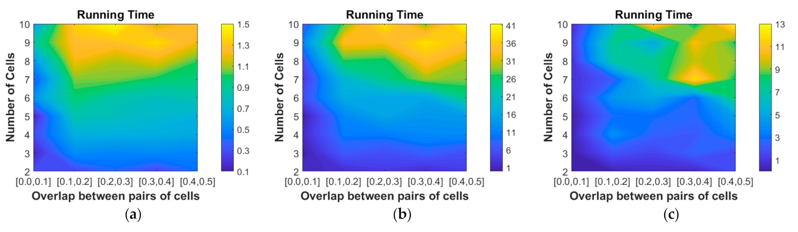
4.2.3. Computational Complexity

We made an average running time comparison between our proposed algorithm and [33] on the test-90 dataset based on the hardware platform with a 2.30 GHz Intel Core i7-4712MQ processor and 12GB DDR3 RAM in the form of an unoptimized MATLAB (The MathWorks, Inc., Natick, MA, USA) code. Figure 10a shows the running time of the initialization described in Section 2.1, which takes 0.14–1.5 min, with an average of 0.79 (std: 0.37) minutes. Figure 10b,c show the running time of [33] and us, respectively, in segmenting cytoplasm contours from the background based on the initialization work. Our proposed algorithm is 2–26 times faster than [33], with an average of 5.4 (std: 4.0) times acceleration for the images on the test-90 dataset. Moreover, when the overlap ratio ranges [0,0.1]–[0.4,0.5], the running time is reduced by 10.4 (std: 6.4), 5.1 (std: 2.7), 4.5 (std: 1.5), 4.1 (std: 1.0) and 3.2 (std: 0.6) times, respectively. When the number of cells ranges 2–10, the running time is reduced by 7.3 (std: 4.2), 3.7 (std: 0.5), 5.3 (std: 3.4), 8.6 (std: 9.6), 5.3 (std: 3.4), 4.2 (std: 2.0), 4.3 (std: 1.6), 5.6 (std: 2.3) and 4.8 (std: 2.6) times.

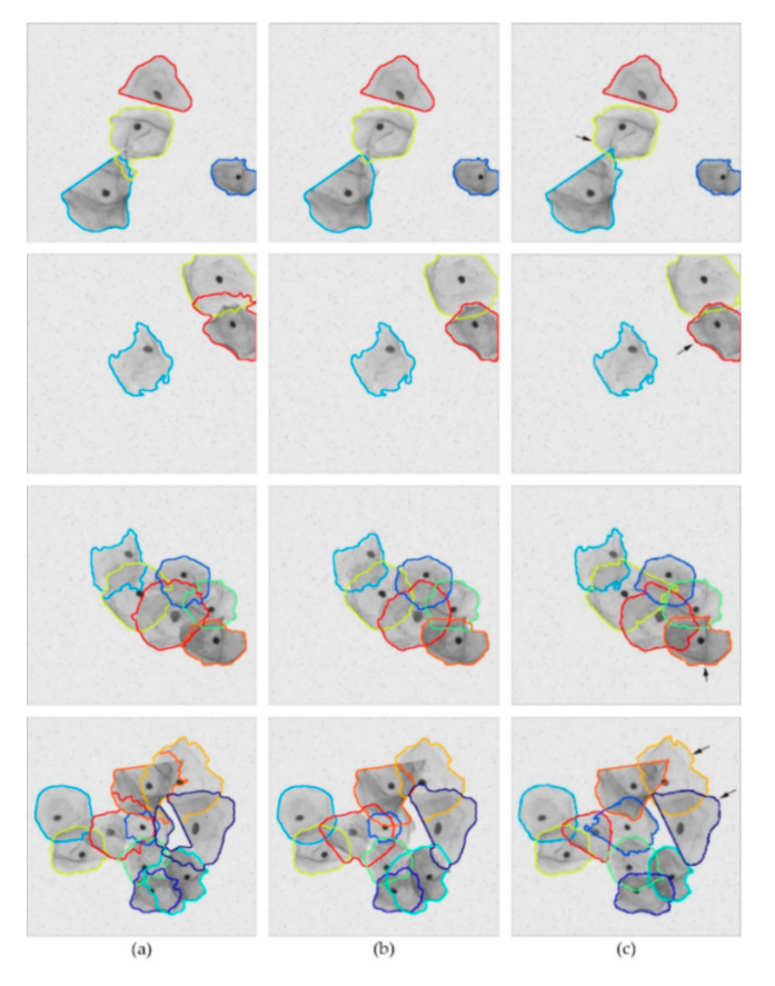
4.3. Qualitative Evaluation of Our Segmentation Results

Four typical segmentations compared with the ground truth and [33] are shown in Figure 11. The improvement can be listed in two aspects: the segmentation for the touching cells and the boundary convergence of the overlapping cells. The pseudo-fragments of the touching cells caused by the misallocation in the initialization of the cellular boundaries can be obviously filtered out by our proposed touching cell splitting algorithm, as shown in the first column of Figure 11. Over-segmentation caused by the absence of an effective guidance mechanism for LSF evolution in [33] is improved by our proposed contour scanning strategy, as shown in the second column of Figure 11. Similarly, the improvement for under-segmentation is shown in the third column of Figure 11. The orange contour and the dark blue contours in the fourth column of Figure 11 further illustrate the improvements by our method.

5. Conclusions

In this paper, we proposed a novel algorithm based on the level set method (LSM) to automatically segment the touching and overlapping cells. The main goal of our proposed method is to address the nonconvergence problem of the baseline method in delineating the overlapping regions of cells, which is caused by ill-defined cytoplasm boundaries in the initialization. Our proposed method exhibits the following contents: (1) we proposed a morphological scaling-based topology filter (MSTF) and a new mathematical toolbox about vector calculus for the evolution of the level set function (LSF). (2) We combined the MSTF and the mathematical toolbox into a multifunctional filtering algorithm DCTLSM that can morphologically scale up and down the contour while keeping part of the contour points fixed. (3) We designed a novel contour scanning strategy for overlapping cell segmentation. The proposed algorithm is capable of fully segmenting cervical cells from the clumps of up to 10 cells with more accurate segmentation. Our segmentation provides an obviously lower false negative rate compared with the baseline method based on the same ill-defined cytoplasm boundaries. By quantitative and qualitive comparison on the ISBI-2014 dataset, our proposed method is superior to other state-of-the-art works.

In the future, our proposed method will be of increasing value in guiding automated slide analyses for cervical pathology after being intertwined with other promising techniques.

References

1. Jemal, A.; Bray, F.; Center, M.M.; Ferlay, J.; Forman, D. Global cancer statistics. Cancer J. Clin. 2011, 6, 169–190. [Google Scholar] [CrossRef] [Green Version]
2. Ferlay, J.; Soerjomataram, I.; Dikshit, R.; Eser, S.; Mathers, C.; Rebelo, M.; Parkin, D.M.; Forman, D.; Bray, F. Cancer incidence and mortality worldwide: Sources, methods and major patterns in globocan 2012. Int. J. Cancer 2012, 136, E359–E386. [Google Scholar] [CrossRef]
3. Bray, F.; Jianlogong, R.; Masuyer, E.; Ferlay, J. Global estimates of cancer prevalence for 27 sites in the adult population in 2008. Int. J. Cancer 2013, 132, 1133–1145. [Google Scholar] [CrossRef]
4. Papanicolaou, G.N. A new procedure for staining vaginal smears. Science 1942, 95, 438–439. [Google Scholar] [CrossRef] [PubMed]
5. American Cancer Society. Cancer Prevention & Early Detection Facts & Figures 2015–2016; American Cancer Society: Atlanta, GA, USA, 2015. [Google Scholar]
6. Pan, X.P.; Li, L.Q.; Yang, H.H.; Liu, Z.B.; Yang, J.X.; Zhao, L.L.; Fan, Y.X. Accurate segmentation of nuclei in pathological images via sparse reconstruction and deep convolutional networks. Neurocomputing 2017, 229, 88–99. [Google Scholar] [CrossRef]
7. Fan, Y.; Bradley, A.P. A method for quantitative analysis of clump thickness in cervical cytology slides. Micron 2016, 80, 73–82. [Google Scholar] [CrossRef] [PubMed] [Green Version]
8. Win, K.P.; Kitjaidure, Y.; Hamamoto, K.; Myo Aung, T. Computer-Assisted Screening for Cervical Cancer Using Digital Image Processing of Pap Smear Images. Appl. Sci. 2020, 10, 1800. [Google Scholar] [CrossRef] [Green Version]
9. Zhang, L.; Kong, H.; Chin, C.T.; Liu, S.; Chen, Z.; Wang, T.; Chen, S. Segmentation of cytoplasm and nuclei of abnormal cells in cervical cytology using global and local graph cuts. Comput. Med. Imaging Graph. 2014, 38, 369–380. [Google Scholar] [CrossRef]
10. Plissiti, M.E.; Nikou, C. A review of automated techniques for cervical cell image analysis and classification. In Biomedical Imaging and Computational Modeling in Biomechanics; Springer-Verlag: Amsterdam, The Netherlands, 2013; Volume 4, pp. 1–18. [Google Scholar]
11. Béliz-Osorio, N.; Crespo, J.M.; García-Rojo, A.M.; Azpiazu, J. Cytology Imaging Segmentation Using the Locally Constrained Watershed Transform. In Proceedings of the 10th International Symposium on Mathematical Morphology and Its Applications to Image and Signal Processing (ISMM 2011), Verbania-Intra, Italy, 6–8 July 2011; Springer-Verlag: Amsterdam, The Netherlands, 2011. [Google Scholar]
12. Bamford, P.; Lovell, B. Unsupervised cell nucleus segmentation with active contours. Signal Process. 1998, 71, 203–213. [Google Scholar] [CrossRef]
13. Jung, C.; Kim, C. Segmenting clustered nuclei using H-minima transform-based marker extraction and contour parameterization. IEEE Trans. Biomed. Eng. 2010, 57, 2600–2604. [Google Scholar] [CrossRef]
14. Plissiti, M.E.; Nikou, C.; Charchanti, A. Watershed-based segmentation of cell nuclei boundaries in Pap smear images. In Proceedings of the IEEE International Conference on Information Technology & Applications in Biomedicine, Corfu, Greece, 3–5 November 2010. [Google Scholar]
15. Jung, C.; Kim, C.; Chae, S.W.; Oh, S. Unsupervised segmentation of overlapped nuclei using Bayesian classification. IEEE Trans. Biomed. Eng. 2010, 57, 2825–2832. [Google Scholar] [CrossRef] [PubMed]
16. Hu, M.; Ping, X.; Ding, Y. Automated cell nucleus segmentation using improved snake. Proc. Int. Conf. Image Process. (ICIP) 2004, 4, 2737–2740. [Google Scholar]
17. Plissiti, M.E.; Nikou, C.; Charchanti, A. Automated detection of cell nuclei in pap smear images using morphological reconstruction and clustering. IEEE Trans. Inf. Technol. Biomed. 2011, 15, 233–241. [Google Scholar] [CrossRef] [PubMed]
18. Plissiti, M.; Charchanti, A.; Krikoni, O.; Fotiadis, D. Automated segmentation of cell nuclei in Pap smear images. In Proceedings of the IEEE International Special Topic Conference on Information Technology in Biomedicine, Ioannina, Greece, 26–28 October 2006; pp. 26–28. [Google Scholar]
19. Lin, C.H.; Chan, Y.K.; Chen, C.C. Detection and segmentation of cervical cell cytoplast and nucleus. Int. J. Imaging Syst. Technol. 2010, 19, 260–270. [Google Scholar] [CrossRef]
20. Yang-Mao, S.F.; Chan, Y.K.; Chu, Y.P. Edge Enhancement Nucleus and Cytoplast Contour Detector of Cervical Smear Images. IEEE Trans. Syst. Man Cybern. 2008, 38, 353–366. [Google Scholar] [CrossRef]
21. Yang, X.; Gao, X.; Tao, D.; Li, X. Improving level set method for fast auroral oval segmentation. IEEE Trans. Image Process. 2014, 23, 2854–2865. [Google Scholar] [CrossRef]
22. Song, Y.; Zhang, L.; Chen, S.; Ni, D.; Lei, B.; Wang, T. Accurate segmentation of cervical cytoplasm and nuclei based on multiscale convolutional network and graph partitioning. IEEE Trans. Biomed. Eng. 2015, 62, 2421–2433. [Google Scholar] [CrossRef]
23. Ushizima, D.; Bianchi, A.; Carneiro, C. Segmentation of Subcellular Compartments Combining Superpixel Representation with Voronoi Diagrams; Tech. Rep. LBNL-6892E; Ernest Orlando Lawrence Berkeley Nat. Lab.: Berkeley, CA, USA, 2015. [Google Scholar]
24. Zhang, L.; Kong, H.; Chin, C.T.; Liu, S.; Fan, T.; Wang, T.; Chen, S. Automation-assisted cervical cancer screening in manual liquid-based cytology with hematoxylin and eosin staining. Cytometry A 2014, 85, 214–230. [Google Scholar] [CrossRef]
25. Ramalho, G.L.; Ferreira, D.S.; Bianchi, A.G.; Carneiro, C.M.; Medeiros, F.N.; Ushizima, D.M. Cell reconstruction under Voronoi and enclosing ellipses from 3D microscopy. In Proceedings of the IEEE International Symposium on Biomedical Imaging (ISBI), Brooklyn Bridge, NY, USA, 16–19 April 2015; pp. 1–2. [Google Scholar]
26. Lee, H.; Kim, J. Segmentation of overlapping cervical cells in microscopic images with superpixel partitioning and cell-wise contour refinement. In Proceedings of the 2016 IEEE Conference on Computer Vision and Pattern Recognition Workshops (CVPRW), Las Vegas, NV, USA, 26 June–1 July 2016; pp. 63–69. [Google Scholar]
27. Kaur, S.; Sahambi, J. Curvelet initialized level set cell segmentation for touching cells in low contrast images. Comput. Med. Imaging Graph. 2016, 49, 46–57. [Google Scholar] [CrossRef]
28. Tareef, A.; Song, Y.; Cai, W.; Feng, D.D.; Chen, M. Automated three-stage nucleus and cytoplasm segmentation of overlapping cells. In Proceedings of the 2014 13th International Conference on Control Automation Robotics & Vision (ICARCV), Singapore, 10–12 December 2014. [Google Scholar]
29. Tareef, A.; Song, Y.; Lee, M.Z.; Feng, D.D.; Cai, W. Morphological Filtering and Hierarchical Deformation for Partially Overlapping Cell Segmentation. In Proceedings of the 2015 International Conference on Digital Image Computing: Techniques and Applications (DICTA), Adelaide, Australia, 23–25 November 2015. [Google Scholar]
30. Nosrati, M.; Hamarneh, G. A variational approach for overlapping cell segmentation. Proc. IEEE ISBI Overlapping Cerv. Cytol. Image Segm. Chall. 2014, 1, 1–2. [Google Scholar]
31. Nosrati, M.; Hamarneh, G. Segmentation of overlapping cervical cells: A variational method with star-shape prior. Proc. ISBI 2015, 186–189. [Google Scholar] [CrossRef]
32. Lu, Z.; Carneiro, G.; Bradley, A.P. Automated nucleus and cytoplasm segmentation of overlapping cervical cells. In Medical Image Computing and Computer-Assisted Intervention; Springer: Berlin, Germany, 2013; pp. 452–460. [Google Scholar]
33. Lu, Z.; Carneiro, G.; Bradley, A. An improved joint optimization of multiple level set functions for the segmentation of overlapping cervical cells. IEEE Trans. Image Process. 2015, 24, 261–272. [Google Scholar]
34. Osher, S.; Sethian, J.A. Fronts propagating with curvature dependent speed: Algorithms based on Hamilton–Jacobi formulations. J. Comput. Phys. 1988, 79, 12–49. [Google Scholar] [CrossRef] [Green Version]
35. Kass, M.; Witkin, A.; Terzopoulos, D. Snakes: Active contour models. Int. J. Comput. Vis. 1988, 1, 321–331. [Google Scholar] [CrossRef]
36. Caselles, V.; Catt´e, F.; Coll, T.; Dibos, F. A Geometric Model for Active Contours in Image Processing. Numer. Math. 1993, 66, 1–31. [Google Scholar]
37. Malladi, R.; Sethian, J.A.; Vemuri, B.C. Shape Modeling with Front Propagation: A Level Set Approach. IEEE Trans. Pami. 1995, 17, 158–175. [Google Scholar] [CrossRef] [Green Version]
38. Mumford, D.; Shah, J. Optimal approximations by piecewise smooth functions and associated variational problems. Commun. Pure Appl. Math. 1989, 42, 577–685. [Google Scholar] [CrossRef] [Green Version]
39. Zhao, H.K.; Chan, T.; Merriman, B.; Osher, S. A Variational Level Set Approach to Multiphase Motion. J. Comput. Phys. 1996, 127, 179–195. [Google Scholar] [CrossRef] [Green Version]
40. Chan, T.; Vese, L. An Active Contour Model without Edges. In International Conference on Scale-Space Theories in Computer Vision; Springer-Verlag: Amsterdam, The Netherlands, 1999. [Google Scholar]
41. Caselles, V.; Kimmel, R.; Sapiro, G. Geodesic active contours. Int. J. Comput. Vis. 1997, 22, 61–79. [Google Scholar] [CrossRef]
42. Chen, Y.; Thiruvenkadam, H.; Tagare, H.; Huang, F.; Wilson, D. On the Incorporation of Shape Priors int Geometric Active Contours. In Proceedings of the IEEE Workshop in Variational and Level Set Methods, Vancouver, BC, Canada, 1 February 2001; pp. 145–152. [Google Scholar]
43. Li, C.M.; Xu, C.Y.; Gui, C.F.; Martin, D.F. Distance regularized level set evolution and its application to image segmentation. IEEE Trans. Image Process. 2010, 19, 3243–3254. [Google Scholar]
44. Canny, J. A Computational Approach to Edge Detection. IEEE Trans. Pattern Anal. Mach. Intell. PAMI 1986, 679–698. [Google Scholar] [CrossRef]
45. Smereka, P. Spiral Crystal Growth. Phys. D Nonlinear Phenom. 2000, 138, 282–301. [Google Scholar] [CrossRef]
46. Burchard, P.; Cheng, L.T.; Merriman, B.; Osher, S. Motion of curves in three spatial dimensions using a level set approach. J. Comput. Phys. 2001, 170, 720–741. [Google Scholar] [CrossRef]
47. Gao, X.; Wang, B.; Tao, D.; Li, X. A relay level set method for automatic image segmentation. IEEE Trans. Syst. Man Cybern. 2011, 41, 518. [Google Scholar]
48. Wang, B.; Gao, X.; Tao, D.; Li, X. A Unified Tensor Level Set for Image Segmentation. IEEE Trans. Syst. Man Cybern. 2010, 40, 857–867. [Google Scholar] [CrossRef]
49. Yang, X.; Gao, X.; Li, J.; Han, B. A shape-initialized and intensity-adaptive level set method for auroral oval segmentation. Inf. Sci. 2014, 277, 794–807. [Google Scholar] [CrossRef]
50. Tareef, A.; Song, Y.; Huang, H.; Wang, Y.; Feng, D.; Chen, M.; Cai, W. Optimizing the cervix cytological examination based on deep learning and dynamic shape modeling. Neurocomputing 2017, 248, 28–40. [Google Scholar] [CrossRef] [Green Version]
51. Huang, Y.; Zhu, H.; Wang, P.; Dong, D. Segmentation of Overlapping Cervical Smear Cells Based on U-Net and Improved Level Set. In Proceedings of the 2019 IEEE International Conference on Systems, Man and Cybernetics (SMC), Bari, Italy, 6–9 October 2019. [Google Scholar]
52. Tareef, A.; Song, Y.; Cai, W.; Huang, H.; Chen, M. Learning Shape-Driven Segmentation Based on Neural Network and Sparse Reconstruction toward Automated Cell Analysis of Cervical Smears. Int. Conf. Neural Inf. Process. 2015, 1, 390–400. [Google Scholar]
53. Tareef, A.; Song, Y.; Cai, W.; Huang, H.; Chang, H.; Wang, Y.; Fulham, M.; Feng, D.; Chen, M. Automatic segmentation of overlapping cervical smear cells based on local distinctive features and guided shape deformation. Neurocomputing 2017, 221, 94–107. [Google Scholar] [CrossRef]
54. Song, Y.Y.; Tan, E.; Jiang, X.D.; Cheng, J.Z.; Ni, D.; Chen, S.P.; Lei, B.; Wang, T. Accurate Cervical Cell Segmentation from Overlapping Clumps in Pap Smear Images. IEEE Trans. Med. Imaging 2017, 36, 288–300. [Google Scholar] [CrossRef]
55. Litjens, G.; Kooi, T.; Bejnordi, B.E.; Setio, A.A.A.; Ciompi, F.; Ghafoorian, M. A survey on deep learning in medical image analysis. Med. Image Anal. 2017, 42, 60–88. [Google Scholar] [CrossRef] [Green Version]
56. Ronneberger, O.; Fischer, P.; Brox, T. U-Net. Convolutional Networks for Biomedical Image Segmentation. In Proceedings of the International Conference on Medical Image Computing and Computer-Assisted Intervention, Munich, Germany, 5–9 October 2015. [Google Scholar]
57. He, K.; Gkioxari, G.; Dollar, P.; Girshick, R. Mask R-CNN. IEEE Trans. Pattern Anal. Mach. Intell. 2018, 42, 386–397. [Google Scholar] [CrossRef]
58. Kirillov, A.; Girshick, R.B.; He, K.; Dollár, P. Panoptic Feature Pyramid Networks. arXiv 2018, arXiv:1901.02446. [Google Scholar]
59. Wan, T.; Xu, S.; Sang, C.; Jin, Y.; Qin, Z. Accurate segmentation of overlapping cells in cervical cytology with deep convolutional neural networks. Neurocomputing 2019, 365, 157–170. [Google Scholar] [CrossRef]
60. Li, K.; Lu, Z.; Liu, W.; Yin, J. Cytoplasm and nucleus segmentation in cervical smear images using radiating GVF snake. Pattern Recognit. 2012, 45, 1255–1264. [Google Scholar] [CrossRef]
61. Kale, A.; Aksoy, S. Segmentation of cervical cell images. In Proceedings of the 2010 20th International Conference on Pattern Recognition, Istanbul, Turkey, 23–26 August 2010; pp. 2399–2402. [Google Scholar]
62. Maurer, C.R.; Qi, R.; Raghavan, V. A linear time algorithm for computing exact euclidean distance transforms of binary images in arbitrary dimensions. IEEE Trans. Pattern Anal. Mach. Intell. 2003, 25, 265–270. [Google Scholar] [CrossRef]
63. Osher, S.; Fedkiw, R. Level Set Methods and Dynamic Implicit Surfaces; Springer: New York, NY, USA, 2003. [Google Scholar]
64. Meyer, F. Topographic distance and watershed lines. Signal Process. 1994, 38, 113–125. [Google Scholar] [CrossRef]
65. Vedaldi, A.; Soatto, S. Quick shift and kernel methods for mode seeking. Comput. Vis. 2008, 705–718. [Google Scholar] [CrossRef] [Green Version]
66. Dillencourt, M.B.; Samet, H.; Tamminen, M. A general approach to connected-component labeling for arbitrary image representations. J. ACM 1992, 39, 253–280. [Google Scholar] [CrossRef]
67. Matas, J.; Chum, O.; Urban, M.; Pajdla, T. Robust wide baseline stereo from maximally stable extremal regions. In Proceedings of the British Machine Vision Conference 2002, Cardiff, UK, 2–5 September 2002; pp. 384–396. [Google Scholar]
68. Osher, S. A Level Set Formulation for the Solution of the Dirichlet Problem for Hamilton–Jacobi Equations. SIAM J. Math. Anal. 1993, 24, 1145–1152. [Google Scholar] [CrossRef]
69. Tsitsiklis, J. Efficient Algorithms for Globally Optimal Trajectories. IEEE Trans. Autom. Control 1995, 40, 1528–1538. [Google Scholar] [CrossRef] [Green Version]
70. Guangqi, L. Mathmatical-Toolbox-for-DCTLSM. Available online: https://github.com/liuchee/Mathmatical-Toolbox-for-DCTLSM (accessed on 1 September 2020).
71. Overlapping Cervical Cytology Image Segmentation Challenge-ISBI. Available online: https://cs.adelaide.edu.au/~carneiro/isbi14_challenge/index.html (accessed on 6 September 2020).
72. Bradley, A.; Bamford, P. A one-pass extended depth of field algorithm based on the over-complete discrete wavelet transform. Image Vis. Comput. N. Z. (IVCNZ) 2004, 1, 279–284. [Google Scholar]
73. Lu, Z.; Carneiro, G.; Bradley, A.; Ushizima, D.; Nosrati, M.; Bianchi, A.G.C.; Carneiro, C.M.; Hamarneh, G. Evaluation of Three Algorithms for the Segmentation of Overlapping Cervical Cells. IEEE J. Biomed. Health Inform. 2017, 21, 441–450. [Google Scholar] [CrossRef]
Figure 1. The architecture of the proposed method takes the contour initialization as the input to perform touching cell splitting (pink arrow) and overlapping cell segmentation (purple arrow). MSTF: morphological scaling-based topology filter and DCTLSM: 2D codimension two-object level set method. The “Fig.” and “Eq.” denote “Figure” and “Equation” respectively.
Applsci 11 00443 g001
Figure 2. Illustration of the algorithm flow of cellular component segmentation. (a) Cervical cytology image; (b) Super-pixel edge map; (c) Clean edge map; (d) Convex hull of cellular clump; (e) Segmentation of cellular clumps; (f) Nuclei detection and segmentation; (g) Initialization of cytoplasm in the cellular clump.
Applsci 11 00443 g002
Figure 3. Process of MSTF and DCTLSM. (a) Misallocated contour fragments; (b) Contour shrunk by MSTF; (c) Contour expanded by MSTF; (d) False negative area; (e) Fixed contour ϕ 0 and active contour ϕ1; (f) Contour shrunk by DCTLSM; (g) Contour expanded by DCTLSM. (h) Refined segmentation by Canny mountain map. TPR: true positive rate, FPR: false positive rate and FNR: false negative rate.
Applsci 11 00443 g003
Figure 4. Explanation of MSTF and DCTLSM. (a) Linear time Euclidean distance transform-signed distance function (LTEDT-SDF) of the initial contour; (b) LTEDT-SDF of the contour shrunk by MSTF; (c) Canny mountain map; (d) Illustration of the morphological shrinking process of the MSTF; (e) Illustration of the morphological expanding process of the MSTF; (f) Illustration of the additional term δ 0 ϕ 1 .
Applsci 11 00443 g004
Figure 5. Process of the segmentation of overlapping cells. (a) Construction of the union contour; (b) Detection of the critical state contour; (c) Discriminant point; (d) Cutting line; (e) Contour scanning result; (f) Contour shrunk by the DCTLSM; (g) Contour expanded by the DCTLSM; (h) Refined segmentation by the Canny mountain map.
Applsci 11 00443 g005
Figure 6. Explanation of the contour scanning strategy. (a) LTEDT−SDF of the union contour; (b) Topology discriminant bridge; (c) Detection of the discriminant point; (d) Velocity field for the evolution of the LSF.
Applsci 11 00443 g006
Figure 7. Selection of the morphological scaling threshold. (a) Numeric outlier detection of the pixel−based average false positive growth rate ( Δ FP ); (b) Validity comparison of the MSTF and DCTLSM with the Δ FP and pixel-based average false negative growth rate ( Δ FN ) at threshold (TH) = 15.
Applsci 11 00443 g007
Figure 8. Illustration of quantitative comparisons in terms of mean the Dice coefficient ( DC ), object−based false negative rate ( FN O ), mean true positive rate ( TP P ), and mean false positive rate ( FP P ) against the baseline method (reproduced from [33], Institute of Electrical and Electronics Engineers, 2015) on the (a) train-45 and (b) test-90 datasets (using the mean and standard deviation results of each measure) at TH = 15. This is a visualization of Table 3.
Applsci 11 00443 g008
Figure 9. Mean Dice coefficient (a), mean true positive rate (b), mean false positive rate (c) and object−based false negative rate (d) as a function of number of cells and overlap ratio.
Applsci 11 00443 g009
Figure 10. Running time (in minutes) of the (a) segmentation of the cellular component (initialization); (b) segmentation of the cytoplasm by the baseline method and (c) segmentation of the cytoplasm by our proposed method.
Applsci 11 00443 g010
Figure 11. Qualitative results of (a) Lu (reproduced from [33], Institute of Electrical and Electronics Engineers, 2015) and (b) our proposed method compared with (c) the ground truth.
Applsci 11 00443 g011