A Fusion Approach to Detect Traffic Signs Using Registered Color Images and Noisy Airborne LiDAR Data

Abstract

Traffic sign detection is considered as one of the active research topics in transportation and computer vision. The previous works mainly focus on detecting traffic signs in images or in mobile light detection and ranging (LiDAR) data. In this paper, we propose a novel deep learning method to accurately detect traffic signs by fusing the complementary features from registered airborne geo-referenced color images and noisy airborne LiDAR data. Specifically, we first segment the airborne color images to road and non-road segments by integrating various local features in an inequality constraint quadratic optimization model. Next, we find the corresponding road regions in LiDAR data and extract high elevated objects above the road. We then segment the extracted objects to different regions corresponding to traffic sign candidates using Euclidean distance-based clustering. Finally, we find the corresponding traffic sign candidates in color images, extract their deep features, and represent them in a convex optimization model to classify the candidates. A set of extensive experiments have been carried out on the airborne geo-referenced color images and noisy airborne LiDAR data captured by Utah State University from I-15 highway. The results show the effectiveness of the proposed method in detecting traffic signs.

1. Introduction

Highway inventory plays a critical role in highway maintenance and asset management. State departments of transportation (DOTs) and local transportation agencies always need up-to-date inventory data to establish the condition of road networks, prioritize reconstruction and repair work, and evaluate highway assets [1]. Traffic signs, as important highway inventory, play an imperative role in road safety and efficiency by giving instructions or providing information to drivers or autonomous vehicles.

Based on the sensing platform, existing highway inventory methods can be classified into two categories: ground-based and air- or space-based methods [1]. Ground-based methods include field inventory, photo/video log, integrated global positioning system (GPS)/global information system (GIS) mapping, terrestrial light detection and ranging (LiDAR), and mobile LiDAR. Air-based methods include aerial/satellite photography and airborne LiDAR. Each method has its advantages and limitations. Recent studies show that the total cost of aerial mapping is much lower than other methods considering the time and personnel needed for large-area inventories (e.g., a whole state highway inventory). As unmanned aerial vehicles (UAVs) become more easily accessible and inexpensive, it is likely that the aerial mapping methods for road inventory will become even less expensive and more efficient in the future.

Here, we introduce several air-based traffic sign detection methods for different types of data captured by different types of sensors. Two common categories of these methods utilize images and light detection and ranging (LiDAR) data. Here, we briefly review several representative approaches that use camera images and LiDAR data.

Several image-based methods have been introduced in recent years to detect and recognize traffic signs. For instance, Soheilian et al. [2] introduce a multi-view constrained 3D reconstruction algorithm, which incorporates color information of traffic signs in imagery data and provides an optimum 3D silhouette for traffic sign detection. Adam and Ioannidis [3] propose to train a support vector machine (SVM) classifier using histogram of oriented gradient (HOG) to detect traffic signs. Khalid et al. [4] extract traffic sign candidates by enhancing the red and blue channel of RGB images based on the assumption that most of the signs are available in these two colors. They further train a SVM-k-nearest neighbor classifier to extract traffic signs among the candidates. Despite the favorable performance of these image-based algorithms, visual features of traffic signs such as color, shape, and appearance are often sensitive to illumination conditions, angles of view, etc.

Recently, researchers have proposed various methods utilizing LiDAR technology for traffic sign detection. However, the number of published work in this aspect is relatively small. Most of these methods use mobile light detection and ranging scanning (MLS) data since they usually have better quality and density than airborne LiDAR. As one of the pioneer works, Pu et al. [5] initially classify the data points to three major categories such as ground surface, objects located on the ground, and objects off the ground. They further incorporate geometrical features including size, shape, and orientation to extract traffic signs from on-ground points. Yokoyama et al. [6] propose to utilize principal component analysis (PCA) to distinguish pole like objects from planar ones in MLS data. In addition, they classify pole like objects into three classes, namely, utility poles, lamp posts, and street signs. Yu and Li [7] eliminate ground points using a voxel-based upward growing method. They then cluster and segment off-ground points into individual objects via Euclidean distance clustering and voxel-based normalized cut segmentation. Riveiro et al. [8] propose to find an optimized intensity threshold in order to segment points corresponding to traffic sign panels. They further perform a contour recognition for each sign using a linear regression model based on a raster image. Lehtomaki et al. [9] utilize prior information to eliminate ground and building points. They then segment the remaining data to different categories based on local descriptor histogram (LDH), spin images, and geometrical features. Javanmardi et al. [10] detect high elevated objects located on top or border of the road in MLS point cloud and cluster these high elevated objects to traffic sign and light pole classes. They further introduce a modified seeded region growing algorithm to remove noisy points and incorporate shape information to filter out false objects from both classes. These aforementioned methods use the 3-dimensional information or reflectiveness of traffic signs to detect various objects. However, their detection efficiency and effectiveness on airborne LiDAR data is degraded due to its low quality resulted from a large number of outliers and different angles of view.

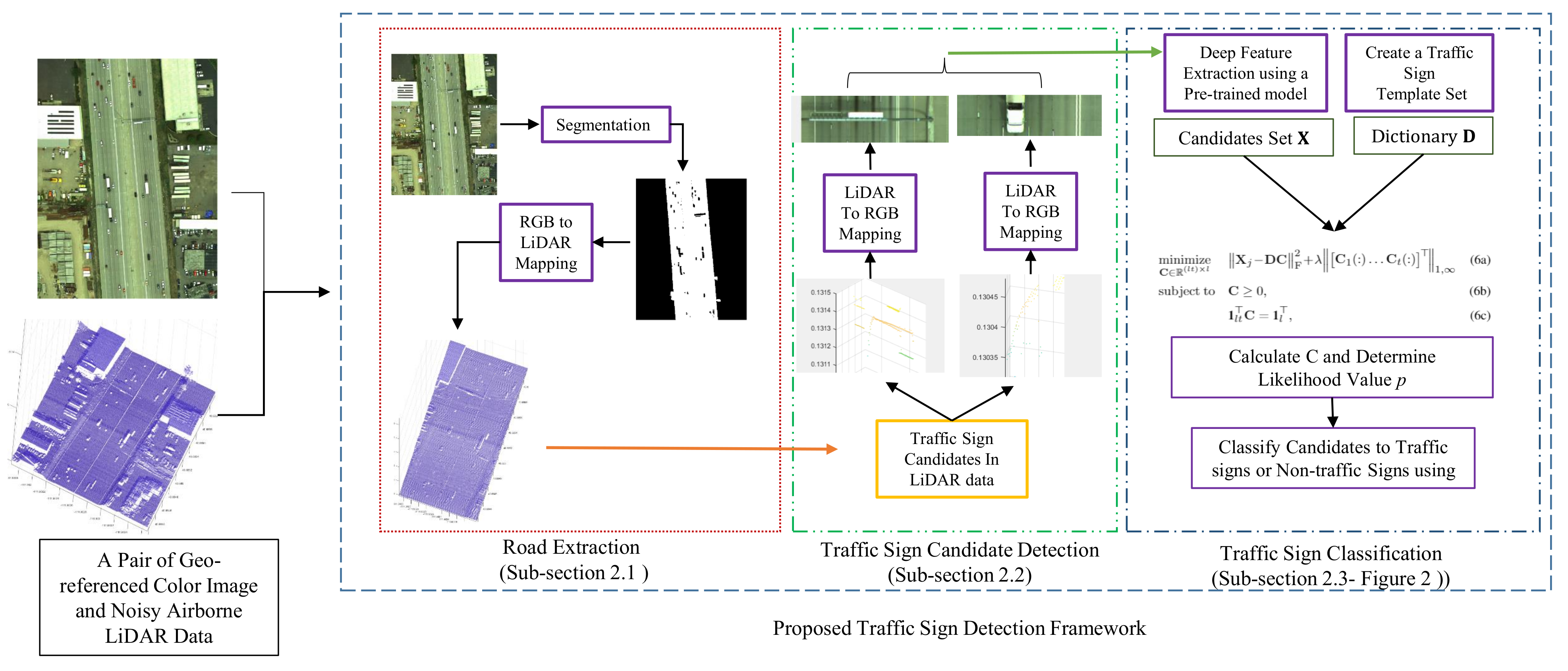
To achieve the maximum level of accuracy and completeness, we propose to develop a data fusion approach that utilizes both aerial LiDAR and aerial imagery data to address the limitations of both image-based and LiDAR-based methods. Unlike other methods [9,10], which detect traffic signs using high resolution MLS data, the proposed method detects traffic sign candidates in airborne LiDAR data, which tend to be more noisy than MLS data and easier and faster to collect. It also represents traffic sign candidates in a convex optimization model in color imagery data to classify candidates as traffic or non-traffic signs at a higher accuracy. Specifically, we first segment the airborne color images to road and non-road segments by integrating various local features in an inequality constraint quadratic optimization model. Next, we find the corresponding road regions in LiDAR data and use the height information to extract high elevated objects above the road. We then use Euclidean distance-based clustering to segment extracted objects into traffic sign candidate regions. Finally, we find the corresponding traffic sign candidate regions in color images and extract their convolutional neural network (CNN) features in a new convex optimization framework to classify them as traffic signs or non-traffic signs. The main contributions of the paper are as follows:

• Incorporating various local features extracted from color imagery data in an inequality constraint quadratic optimization model and numerically solving the model using the accelerated proximal gradient (APG) method.
• Adopting Euclidean distance-based clustering to classify high elevated objects in LiDAR data to several object candidates.
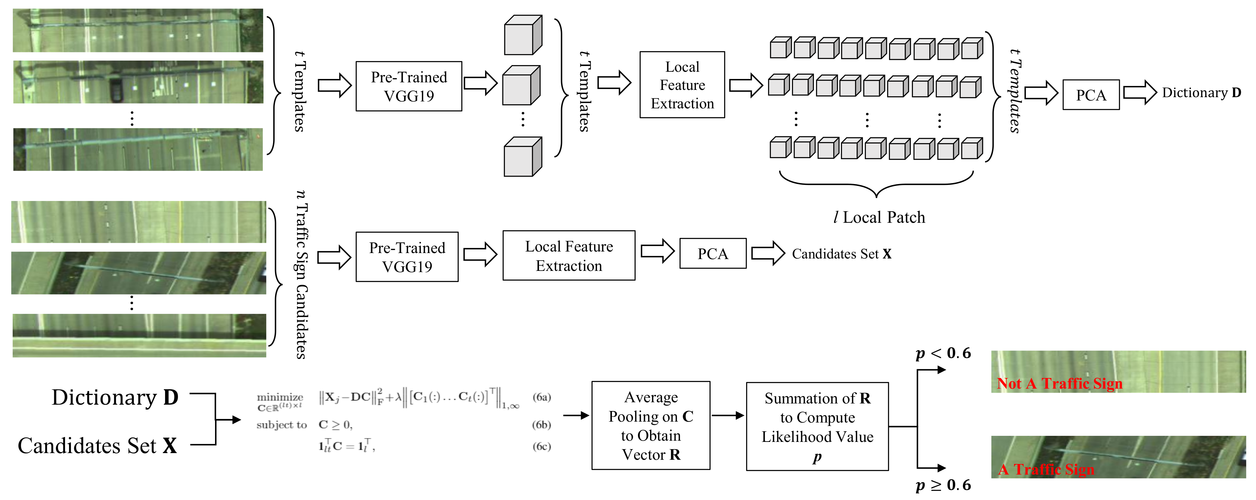
• Developing a convex optimization model in color imagery data to classify object candidates as traffic or non-traffic signs.
• Seamlessly combining the CNN features of local patches of each object candidate with a group-sparsity regularization term to encourage the classifier to sparsely select appropriate local patches of the same subset of templates.
• Designing a fast and parallel numerical algorithm by deriving the augmented Lagrangian of the optimization model into two close-form problems: the quadratic problem and the Euclidean norm projection onto probability simplex constraints problem.

The remainder of this paper is organized as follows: Section 2 describes the three main components of the proposed method in detail. These three components are road extraction, traffic sign candidate detection, and traffic sign classification. Section 3 presents experimental results and demonstrates the effectiveness of the proposed method to utilize information captured from geo-referenced color images and noisy airborne LiDAR data provided by Utah State University (USU) for Utah DOT (UDOT) along I-15 highway. Section 4 draws the conclusions.

2. Proposed Method

The proposed method incorporates the complimentary information captured from airborne color images and noisy airborne LiDAR data to accurately detect traffic signs in highway areas. To this end, it first utilizes geo-referenced color images to remove non-road points and keep candidate road points as the search space, which significantly reduces the time spent in searching for traffic sign candidates. It then maps the reduced search space in color images to its corresponding reduced search space in LiDAR data to quickly detect traffic sign candidates using the height information. Finally, it maps traffic sign candidates in LiDAR data to their counterparts in color images, employs the deep learning technique to automatically extract deep features, and uses the deep features in the optimization model to classify traffic sign candidates as positive or negative. These three major steps are summarized in the diagram as presented in Figure 1, where we name each step as road extraction, traffic sign candidate detection, and traffic sign classification, respectively. Detailed information about each step is presented in Section 2.1, Section 2.2 and Section 2.3.

2.1. Road Extraction

Since traffic signs are located above road areas, we aim to remove non-road pixels from color images to reduce the search space to exclusively contain road pixels. We employ an image segmentation technique [11] to extract and integrate complementary local features of a group of image pixels in a factorization-based framework. This framework builds multiple representations of image pixels, which are represented in an optimization model to obtain more informative representation of image pixels for segmentation. We then manually select pixels from road and non-road regions and respectively construct two dictionaries from these pixels to store the feature information of road and non-road regions. The feature of a candidate pixel is finally represented by the road and non-road dictionaries in quadratic optimization problems with equality constraints to classify it as either road or non-road. We explain the type of extracted features in Section 3.1. We denote the two dictionaries, which store the features of road and non-road regions, as road dictionary and non-road dictionary, respectively. We classify the candidate pixels that are well presented by the road dictionary in the quadratic optimization problem with equality constraints (i.e., the reconstruction error with respect to road dictionary is less than the reconstruction error with respect to non-road dictionary) as road regions.

To do so, we over-segment each image to extract $n_{os}$ segments (super-pixels) [12]. We then construct $n_f$ feature matrices with each containing one kind of feature with a dimension of $d_w$ for all $n_{os}$ segments. For the wth feature matrix ${\mathbf{Y}}^w\in R^{d_w\times n_{os}}$, we model it as follows:

$${\mathbf{Y}}^w={\mathbf{T}}^w{\mathbf{Z}}^w+{\mathbf{E}}^w$$

(1)

where ${\mathbf{T}}^w\in R^{d_w\times n_k}$ is a dictionary of $n_k$ words with a dimension of $d_w$, ${\mathbf{Z}}^w\in R^{n_k\times n_{os}}$ is a new representation of the features of all segments using $n_k$ dictionary words, and ${\mathbf{E}}^w$ is the model error. In the segmentation task, we aim to learn ${\mathbf{Z}}^w$ by adopting non-negative matrix factorization in the following optimization model:

$$\begin{array}{cc}\hfill \underset{{\mathbf{T}}^w,{\mathbf{Z}}^w}{minimize}& {∥{\mathbf{Y}}^w-{\mathbf{T}}^w{\mathbf{Z}}^w∥}_{\mathrm{F}}^2\hfill \end{array}$$

(2a)

$$\begin{array}{cc}\hfill \mathrm{subject} \mathrm{to}& {\mathbf{Z}}^w\ge 0,{\mathbf{T}}^w\ge 0\hfill \end{array}$$

(2b)

We use the alternating least square (ALS) method [13] to solve this optimization problem for all feature matrices ${\mathbf{Y}}^w(w=1,\cdots ,n_f$). Calculated representation matrices ${\mathbf{Z}}^w(w=1,\cdots ,n_f$) contain $n_f$ kinds of complementary feature information of $n_{os}$ segments. As a result, they are more informative than one matrix containing individual feature [11].

We use a linear combination of matrices ${\left\{Z^w\right\}}_{w=1}^{n_f}$ to model $\mathbf{Q}$ to represent the final segmentation results. The coefficients of such a linear combination are gathered into a vector $\mathbf{p}\in R^{n_f\times 1}$ to measure the reliability of representations. We formulate the following aggregation model to compute $\mathbf{Q}$:

$$\begin{array}{c}\hfill \begin{array}{cc}\underset{\mathbf{Q},\mathbf{p}}{minimize}\hfill & {∥{\displaystyle \sum _{i=1}^{n_f}}{\mathbf{p}}_i{\mathbf{Z}}^i-\mathbf{Q}∥}_{\mathrm{F}}^2+\gamma Tr\left(\mathbf{Q}\mathbf{L}{\mathbf{Q}}^{\top }\right)\hfill \end{array}\end{array}$$

(3a)

$$\begin{array}{c}\hfill \begin{array}{cc}\mathrm{subject} \mathrm{to}\hfill & \mathbf{p}\ge 0,{\mathbf{1}}^T\mathbf{p}=1\hfill \end{array}\end{array}$$

(3b)

where $\mathbf{1}$ is a ones column vector, $\gamma$ is a regularization parameter, $\mathbf{L}$ is a Laplacian matrix, and $Tr(·)$ is the trace operator. The Laplacian matrix L is constructed over a graph $\mathcal{G}$, where its nodes are segments and its edges connect the neighboring segments [11]. The first term is the penalization of representing the violation of the linear model. The second term is the Laplacian regularization term, which considers effect of each segment’s vicinity in the objective function and attains the smoothness of $\mathbf{Q}$ with respect to matrix $\mathbf{L}$.

For the final learning step, we manually select $n_{sf}$ pixels from road regions and $n_{sf}$ pixels from non-road regions of two training images of the geo-referenced color image set. We then extract $n_f$ kinds of features (${\mathbf{Y}}^w\in R^{d_w\times n_{sf}},w=1,\dots ,n_f$) for the region around each of these manually selected pixels. These feature types will be explained in Section 3.1. We next use Equations (2) and (3) to obtain respective feature representations, $\mathbf{Q}$s, for the $n_{sf}$ road and $n_{sf}$ non-road pixels. The two vectorized $\mathbf{Q}$s are used to form the dictionaries, namely, ${\mathbf{D}}_r\in R^{d_f\times n_{sf}}$ (road dictionary) and ${\mathbf{D}}_{nr}\in R^{d_f\times n_{sf}}$ (non-road dictionary). Here, $d_f$ is the dimension of the vectorized feature representation $\mathbf{Q}$. Finally, the feature vector ($\mathbf{x}\in R^{d_f\times 1}$) of a candidate pixel is represented by ${\mathbf{D}}_r$ and ${\mathbf{D}}_{nr}$ in two similar quadratic optimization problems with equality constraints, which can be solved analytically by writing the KKT conditions [14]. The candidate pixel, $\mathbf{x}$, is classified as road if the reconstruction error with respect to dictionary ${\mathbf{D}}_r$ is less than the reconstruction error with respect to dictionary ${\mathbf{D}}_{nr}$. Otherwise, it is classified as non-road.

2.2. Traffic Sign Candidate Detection

In order to remove obvious non-traffic signs above road areas, we utilize the height (z) information of extracted road points in the LiDAR data to obtain traffic sign candidates. We perform the following steps to filter out the road and low elevated objects and extract traffic sign candidate regions:

• Employ the image to global coordinate projection on road regions extracted from each color image to find their corresponding road regions in its geo-referenced LiDAR data. The projection is performed by using six affine parameters to map the road pixel i at location $(x_i,y_i)$ in an image to its associated point l at location $(x_l,y_l)$ in LiDAR data.
• Calculate the histogram of the height values $z^{\prime }s$ of extracted road points in LiDAR data.
• Find the center of the histogram bin with the maximum number of points and set this center value as the threshold $T_z$.
• Filter out the points whose z values are less than $T_z+T_0$, where $T_0$ is an empirically determined offset value to remove vehicles or any low elevated objects on the road.
• Use the Euclidean distance-based clustering algorithm to segment remaining high elevated objects to traffic sign candidates.
• Remove small traffic sign candidates containing less than $T_1$ points.
• Employ the global to image coordinate projection on traffic sign candidates extracted from each geo-referenced airborne LiDAR data to find their counterparts in its color image. This projection is the inverse of the image to global coordinate projection.

It should be noted that the two thresholds, $T_0$ and $T_1$, have to be empirically determined based on the resolution and density of the LiDAR data set. We use the image to global coordinate projection as defined in Equation (4) to map a pixel i at location $(x_i,y_i)$ in an image to its associated point l at location $(x_l,y_l)$ in LiDAR data.

$$\left[\begin{array}{c}{x}_l\\ y_l\end{array}\right]=\left[\begin{array}{ccc}R\left(0\right)& R\left(1\right)& R\left(2\right)\\ R\left(3\right)& R\left(4\right)& R\left(5\right)\end{array}\right]\left[\begin{array}{c}{x}_i\\ y_i\\ 1\end{array}\right]$$

(4)

We use the global to image coordinate projection as defined in Equation (5) to map a point l at location $(x_l,y_l,z_l)$ in LiDAR data to its associated pixel i at location $(x_i,y_i)$ in image data.

$$\left[\begin{array}{c}{x}_i\\ y_i\\ 1\end{array}\right]={\left[\begin{array}{ccc}R\left(0\right)& R\left(1\right)& R\left(2\right)\\ R\left(3\right)& R\left(4\right)& R\left(5\right)\\ 0& 0& 1\end{array}\right]}^{-1}\left[\begin{array}{c}{x}_l\\ y_l\\ z_l\end{array}\right]$$

(5)

where $R\left(0\right)=0.0,R\left(1\right)=-0.076,R\left(2\right)=0.079,R\left(3\right)=0.0,R\left(4\right)=4.230\times {10}^5,$ and $R\left(5\right)=4.506\times {10}^5$.

2.3. Traffic Sign Classification

Inspired by [15], we propose a deep-features-based sparse classifier to recognize traffic sign candidates. This classifier employs CNN deep features of the local patches within a traffic sign candidate and represents them using a template set consisting of local deep features of traffic signs. In Section 2.3.1, we present the formulation of the proposed sparse classifier optimization model. In Section 2.3.2, we describe the numerical algorithm to solve the sparse classifier model. In Section 2.3.3, we explain the details to extract the local deep features of traffic sign candidates and traffic sign templates. In Section 2.3.4, we present the overview of the sparse classifier optimization model.

2.3.1. Sparse Classifier Optimization Model

In order to classify traffic signs, we choose t traffic sign templates from the color image set. We select l pre-determined overlapping local patches inside each traffic sign template to ensure some important features of the traffic sign are captured in each patch and all important features of the traffic sign are captured by all patches. We then employ the CNN to extract a d-dimensional deep feature vector for each patch. These feature vectors are utilized to construct the template set $\mathbf{D}=[{\mathbf{D}}_1,\cdots ,{\mathbf{D}}_t]\in {\mathbb{R}}^{d\times \left(lt\right)}$, where ${\mathbf{D}}_i\in {\mathbb{R}}^{d\times l}$.

For each of n traffic sign candidates in color images, we select the same l pre-determined overlapping local patches within itself and employ the CNN to extract a d-dimensional deep feature vector for each patch. Using these l feature vectors, we build the traffic sign candidate matrix $\mathbf{X}=[{\mathbf{X}}_1,\cdots ,{\mathbf{X}}_n]\in {\mathbb{R}}^{d\times \left(ln\right)}$. We denote the sparse coefficient matrix corresponding to the jth traffic sign candidate as $\mathbf{C}\triangleq {\left[\begin{array}{ccc}{\mathbf{C}}_1& \cdots & {\mathbf{C}}_t\end{array}\right]}^{\top }\in {\mathbb{R}}^{\left(lt\right)\times l}$, where ${\left\{{\mathbf{C}}_q\right\}}_{q=1}^t$ is an $l\times l$ matrix indicating the group representation of l local features of the jth traffic sign candidate using l local features of the qth traffic sign template ($q=1\cdots t$). We formulate the following convex model to represent deep features of the jth traffic sign candidate using t traffic sign templates in a set:

$$\underset{\mathbf{C}\in {\mathbb{R}}^{\left(lt\right)\times l}}{\mathrm{minimize}}\hspace{1em}{∥{\mathbf{X}}_j-\mathbf{D}\mathbf{C}∥}_{\mathrm{F}}^2+\lambda {∥{\left[\begin{array}{c}{\mathbf{C}}_1(:)\dots {\mathbf{C}}_t(:)\end{array}\right]}^{\top }∥}_{1,\infty }$$

(6a)

$$\begin{array}{c}\mathrm{subject} \mathrm{to}\hspace{1em}\mathbf{C}\ge 0,\hfill \end{array}$$

(6b)

$${\mathbf{1}}_{lt}^{\top }\mathbf{C}={\mathbf{1}}_l^{\top },$$

(6c)

The first term in (6a) shows the similarity between a traffic sign candidate matrix ${\mathbf{X}}_j$ and the traffic sign template set. The second term is a group-sparsity regularization term, which penalizes the objective function in proportion with the number of selected templates. It establishes the ${∥·∥}_{1,\infty }$ minimization on matrix $\mathbf{C}$ to impose all local patches inside a candidate to jointly select similar few templates. Particularly, the $l_1$ norm minimization on the columns of $\mathbf{C}$ makes them to be sparse and therefore selects few traffic sign templates for representation. The $l_{\infty }$ norm minimization on the rows of $\mathbf{C}$ motivates the group of local patches to jointly select similar few templates. The parameter $\lambda >0$ is a trade-off to balance the two terms. The constraint (6b) ensures sparse coefficients to be non-negative since a traffic sign candidate may be represented by traffic sign templates dominated by non-negative coefficients. The constraint (6c) ensures that at least one local patch of the template set is selected to represent a local patch in ${\mathbf{X}}_j$.

2.3.2. Numerical Algorithm

To find the sparse representation, $\mathbf{C}$, of each traffic sign candidate in (6), we provide a fast numerical solution based on the alternating direction method of multipliers (ADMM) [16]. To do so, we introduce auxiliary variables in the objective function to simplify the optimization model and derive its augmented Lagrangian.

We define a vector $\mathbf{m}\in {\mathbb{R}}^t$ such that ${\mathbf{m}}_i=\mathrm{argmax}|{\mathbf{C}}_i(:)|$ and replace the second term of (6a) with $\lambda {\mathbf{1}}_t^{\top }\mathbf{m}$. To ensure the equivalence of optimization problems, we impose $\mathbf{m}\otimes {\mathbf{1}}_l{\mathbf{1}}_l^{\top }\ge \mathbf{C}$ as an inequality constraint and provide a non-negative slack matrix $\mathbf{U}\in {\mathbb{R}}^{\left(lk\right)\times l}$ to compensate the difference between the two sides of this inequality constraint. Therefore, $\mathbf{m}\otimes {\mathbf{1}}_l{\mathbf{1}}_l^{\top }=\mathbf{C}+\mathbf{U}$. After this simplification, we write the augmented Lagrangian as:

$$\begin{array}{c}{\mathcal{L}}_{\mu }(\mathbf{C},\mathbf{U},\hat{\mathbf{C}},\hat{\mathbf{U}},{\mathbf{\Lambda }}_1,{\mathbf{\Lambda }}_2)={∥{\mathbf{X}}_j-\mathbf{D}\mathbf{C}∥}_{\mathrm{F}}^2+\frac{\lambda }{l^2}{\mathbf{1}}_{\left(lt\right)}^{\top }(\mathbf{C}+\mathbf{U}){\mathbf{1}}_l\\ +\frac{{\mu }_1}{2}{∥\mathbf{C}-\hat{\mathbf{C}}+\frac{{\mathbf{\Lambda }}_1}{{\mu }_1}∥}_{\mathrm{F}}^2+\frac{{\mu }_2}{2}{∥\mathbf{U}-\hat{\mathbf{U}}+\frac{{\mathbf{\Lambda }}_2}{{\mu }_2}∥}_{\mathrm{F}}^2\end{array}$$

(7)

where $\mathbf{U}\in {\mathbb{R}}^{\left(lk\right)\times l}$ is a non-negative slack matrix, $\hat{\mathbf{C}}$ and $\hat{\mathbf{U}}$ are auxiliary variables with the same dimension as $\mathbf{U}$, ${\mu }_1$ and ${\mu }_2$ are positive augmented Lagrangian parameters, and ${\mathbf{\Lambda }}_1,{\mathbf{\Lambda }}_2\in {\mathbb{R}}^{\left(lt\right)\times l}$ are the Lagrangian multipliers. Without loss of generality, we assume ${\mu }_1={\mu }_2=\mu$. Given an initialization for $\hat{\mathbf{C}}$, $\hat{\mathbf{U}}$, ${\mathbf{\Lambda }}_1$, and ${\mathbf{\Lambda }}_2$, the ADMM method is used to solve (7) via multiple iterations:

$$\begin{array}{c}\hfill \begin{array}{ccc}({\mathbf{C}}^{i+1},{\mathbf{U}}^{i+1}):=\hfill & \underset{\mathbf{C},\mathbf{U}\in {\mathbb{R}}^{\left(lt\right)\times l}}{\arg \min }\hfill & {\mathcal{L}}_{\mu }(\mathbf{C},\mathbf{U},{\hat{\mathbf{C}}}^t,{\hat{\mathbf{U}}}^i,{\mathbf{\Lambda }}_1^i,{\mathbf{\Lambda }}_2^i)\hfill \\ & \mathrm{subject} \mathrm{to}\hfill & \mathbf{E}(\mathbf{C}+\mathbf{U})=\frac{{\mathbf{I}}_t\otimes {\mathbf{1}}_l{\mathbf{1}}_l^{\top }}{l}(\mathbf{C}+\mathbf{U})\hfill \end{array}\end{array}$$

(8)

$$\begin{array}{c}\hfill \begin{array}{ccc}({\hat{\mathbf{C}}}^{i+1},{\hat{\mathbf{U}}}^{i+1}):= \hfill & \underset{\mathbf{C},\mathbf{U}\in {\mathbb{R}}^{\left(lt\right)\times l}}{\arg \min }\hfill & {\mathcal{L}}_{\mu }({\mathbf{C}}^{i+1},{\mathbf{U}}^{i+1},\hat{\mathbf{C}},\hat{\mathbf{U}},{\mathbf{\Lambda }}_1^i,{\mathbf{\Lambda }}_2^i)\hfill \\ & \mathrm{subject} \mathrm{to}\hfill & \hat{\mathbf{C}}\ge 0\hfill \\ & & {\mathbf{1}}_{\left(lt\right)}^{\top }\hat{\mathbf{C}}={\mathbf{1}}_l^{\top }\hfill \\ & & \hat{\mathbf{U}}\ge 0\hfill \end{array}\end{array}$$

(9)

$$\begin{array}{cc}\hfill & {\mathbf{\Lambda }}_1^{i+1}={\mathbf{\Lambda }}_1^i+\mu ({\mathbf{C}}^{i+1}-{\hat{\mathbf{C}}}^{i+1})\hfill \\ \hfill & {\mathbf{\Lambda }}_2^{i+1}={\mathbf{\Lambda }}_2^i+\mu ({\mathbf{U}}^{i+1}-{\hat{\mathbf{U}}}^{i+1})\hfill \end{array}$$

(10)

To solve (8), we first stack the ith rows of $\mathbf{C}$ and $\mathbf{U}$ and construct ${\left\{{\mathbf{z}}_i\right\}}_{i=1}^{lt}$, where ${\mathbf{z}}_i\in {\mathbb{R}}^{2l}$. We then divide (8) into $lt$ equality constrained quadratic problems. Each problem is solved analytically by writing Karush–Kuhn–Tucker (KKT) conditions. Using the solution of (8), we solve the optimization problem in (9) by splitting it into two separate subproblems. The first subproblem is over $\hat{\mathbf{C}}$ and consists of l independent Euclidean norm projections onto the probability simplex. The second subproblem is over $\hat{\mathbf{U}}$ and consists of l independent Euclidean norm projections onto the non-negative orthant. We finally update ${\mathbf{\Lambda }}_1$ and ${\mathbf{\Lambda }}_2$ in (10) by performing l parallel updates over their respective columns. The three iterative steps as detailed in (8)–(10) can be quickly run due to their closed form solutions.

2.3.3. Local Deep Feature Extraction

Convolutional Neural Networks (CNNs) have recently been applied to various computer vision tasks such as image classification [17,18], semantic segmentation [19,20], object detection [21], and object tracking [22,23,24]. The robustness of CNN deep features is mostly due to their outstanding performance in representing visual data compared to hand-crafted features. Taking advantages of deep learning, we extract the deep features of traffic sign candidates and traffic sign templates using a pre-trained network (VGG-Net 19 [20]), which is trained on the ImageNet [25] dataset. This dataset contains more than one million images categorized into 1000 classes. Specifically, we perform the following steps: (1) resize traffic sign candidates to $112\times 112\times 3$; (2) pass the resized traffic sign candidates to the VGG-Net 19; (3) extract the feature maps from layer Conv 5-4 and resample them to the size of $28\times 28\times 512$; (4) construct nine local feature maps with the size of $14\times 14\times 512$ using the stride of 7; (5) Flatten each local feature map into a vector and perform PCA to obtain top 1120 features.

2.3.4. Summary

Figure 2 presents an overview of the proposed deep-features-based sparse classifier optimization model. We first construct a dictionary $\mathbf{D}$ to represent the characteristic features of traffic signs. This dictionary is constructed from l deep features extracted from overlapping local patches inside each of t traffic sign templates chosen from the color image set. To make a compact dictionary, we employ the PCA method to keep the 1120 most important features from the $14\times 14\times 512=$ 100,352 dimensional deep feature vector extracted from the pre-trained VGG-Net 19. Each traffic sign candidate ${\mathbf{X}}_j$ is passed down to the pre-trained VGG-Net 19 to extract local deep features, which are further compressed by PCA. Its corresponding sparse matrix $\mathbf{C}$ is computed based on the proposed optimization model (6a). In order to classify each target candidate using its corresponding $\mathbf{C}$, we apply average pooling on $\mathbf{C}$ and obtain a representative vector $\mathbf{R}$ for each traffic sign candidate [26]. The summation of the representative vector, $\mathbf{R}$, is used as a likelihood value p. Candidates with a likelihood value (p) larger than a predefined threshold are considered as traffic signs.

3. Experimental Results

We evaluated the performance of the proposed local deep-features-based traffic sign detection method by conducting various experiments on 20 sections of multiple pairs of airborne color images and noisy LiDAR data collected from I-15 highway located in Utah, United States (e.g., I-15 North mileposts 284 to 307 and I-15 South mileposts 241 to 260). Airborne LiDAR data were collected by the Remote Sensing Service Laboratory (RSSL) at Utah State University (USU). The USU airborne LiDAR system was mounted in a single engine Cessna TP206 aircraft. The system consisted of a LiDAR scanner, inertial measurement unit (IMU), and flight navigation unit. This LiDAR instrument was composed of a Riegl Q560 transceiver and Novatel SPAN LN-200 GPS/IMU positioning and orientations system. Depending on the flight height, the LiDAR scanner could collect data at a pulse rate of 250,000 shots/s. The beam divergence was less than 0.5 mrad, which allows the LiDAR scanner to have a footprint of about 0.5 m at flight height of 1000 m above ground level (agl). Each section of the roads of interests was divided into multiple subsections, with each covered by a single flight line. The data were acquired at an average flight height of approximately 500 m agl or lower. The LiDAR scan rate was about 125 Hz, the pulse rate was 200,000 shots/s, and the average flight speed was about 180 km/h. In these settings, the point density of the LiDAR data could be up to 6.2 points/m${}^2$ [1].

The UDOT provided the locations of traffic signs for each dataset. We used these locations to find the corresponding regions in the color images and cropped them as ground-truth for traffic signs. The quantitative evaluation of the proposed method was based on the traffic sign locations provided by the UDOT. If the detection result and the ground truth overlap, we considered it as true positive. It should be also noted that the data in the collected 20 sections contained different traffic flows since it was collected along the I-15 highway for 40 miles. It would be nice to collect data under multiple conditions including different traffic flows, different days and times, and different weather conditions to thoroughly test the performance of the proposed method. However, collecting data under these circumstances takes time and effort.

In Section 3.1, we provide road extraction results on 20 sections of the road on color images. In Section 3.2, we provide traffic sign candidate extraction and classification results on the same 20 sections of the road. Due to the lack of space, we qualitatively show eight representative sections of the road and present the quantitative results of all 20 sections for evaluation. In Section 3.3, we compare the performance of the proposed traffic sign detection method with several state-of-the-art methods.

3.1. Road Extraction Results

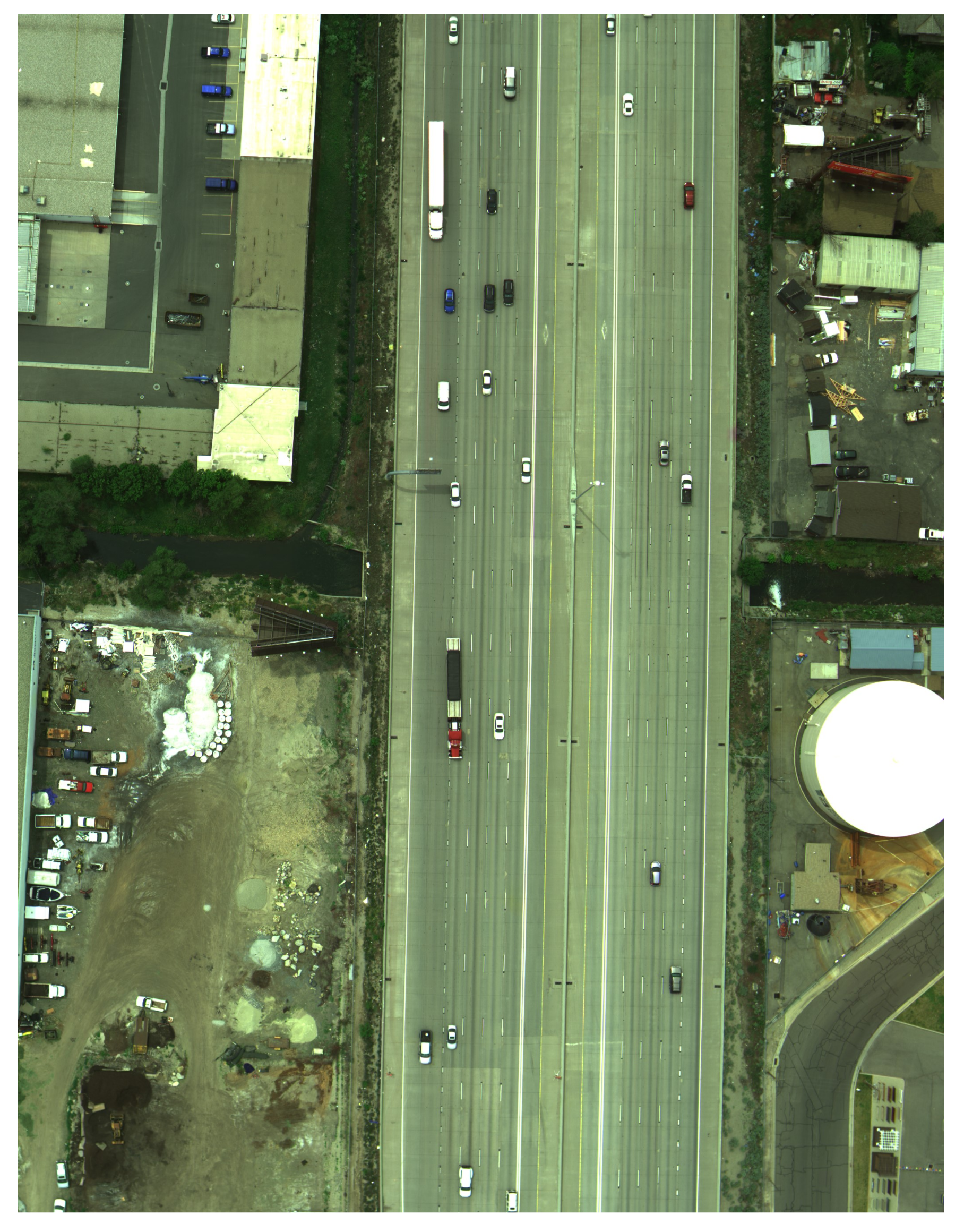
To evaluate the performance of the proposed road extraction method, we conducted extensive experiments on 20 sections of the road. Each section section(i) ($i=1,\cdots ,20$) contained different kinds of objects such as road, buildings, vegetation, parking lots, etc. Figure 3 demonstrates section(1) of a geo-referenced color image of the dataset that contains objects such as road, vehicles, building, and vegetation commonly seen on a highway.

We generated six feature matrices from over-segmented regions [27] of the input image on six sets of complementary layers [11], which represented the input image from different perspectives. The six sets of layers included color layers of CIE-LAB and $Y{C}_b{C}_r$ color spaces, gradient layers of Gaussian and Laplacian of Gaussian, soft segmentation layers [28] of first three principal components, a texture layer [29], a combined color and soft segmentation layer, and a combined color, gradient, soft segmentation, and texture layer. We then extracted local spectral histogram (LSH) for image pixels from each of the six layers. A feature vector by averaging features of all pixels within a region represented characteristic features of the region. The feature vectors for each over-segmented region were combined to construct the corresponding feature matrix. For the last step of road and non-road extraction, we extracted the aforementioned local features for $n_{sf}$ pixels in road regions and construct the road dictionary. Similarly, we built the non-road dictionary by extracting the local features for $n_{sf}$ pixels in non-road regions. For all experiments, we set $\gamma$ in (3a) as 10 to control the smoothness of the result.

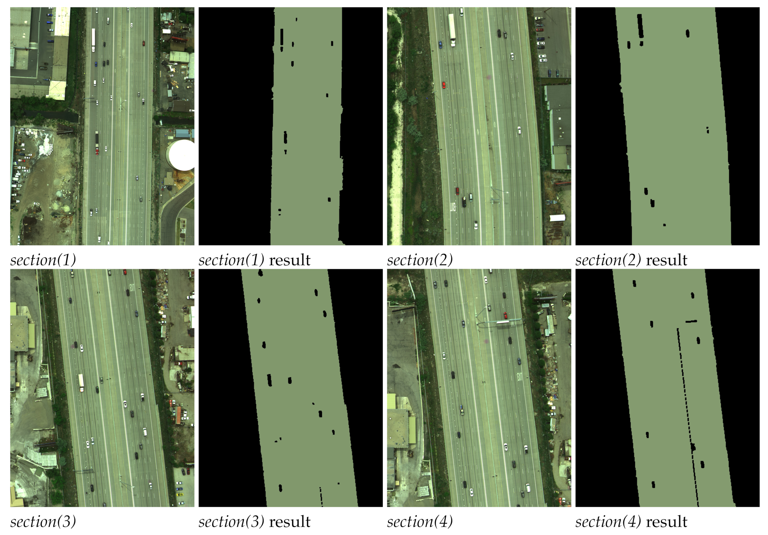
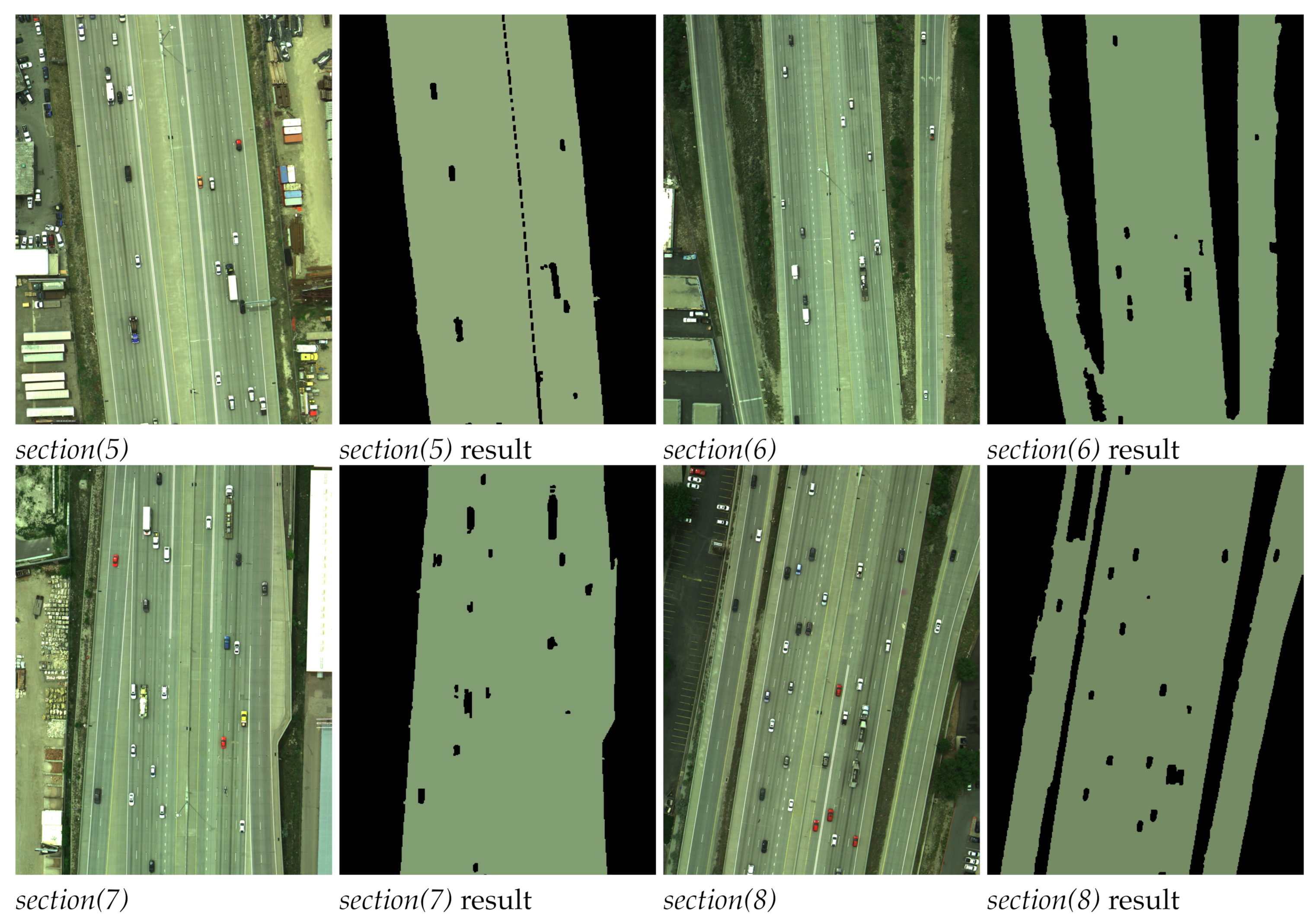
We qualitatively demonstrated road extraction results on four sections of the road (i.e., section(1), section(2), section(3), and section(4)) in Figure 4 and another four sections of the road (i.e., section(5), section(6), section(7), and section(8)) in Figure 5. The section(1) and section(2) in Figure 4 demonstratde the conditions with low traffic flows while section(7) and section(8) in Figure 5 demonstrated the conditions with high traffic flows. The section(6) and section(8) in Figure 5 had road bypass with vegetation in between. The section(1), section(3), and section(4) in Figure 4 had buildings along the road and section(2) had the highest vegetation along the road among all the demonstrated sections. The road extraction results for all sections shown in Figure 4 and Figure 5 clearly demonstrated the robustness of the proposed method in extracting road regions under multiple conditions including different traffic flows, different road-side buildings, various road shapes, and various road-side objects (i.e., vegetation, building, and parking lot).

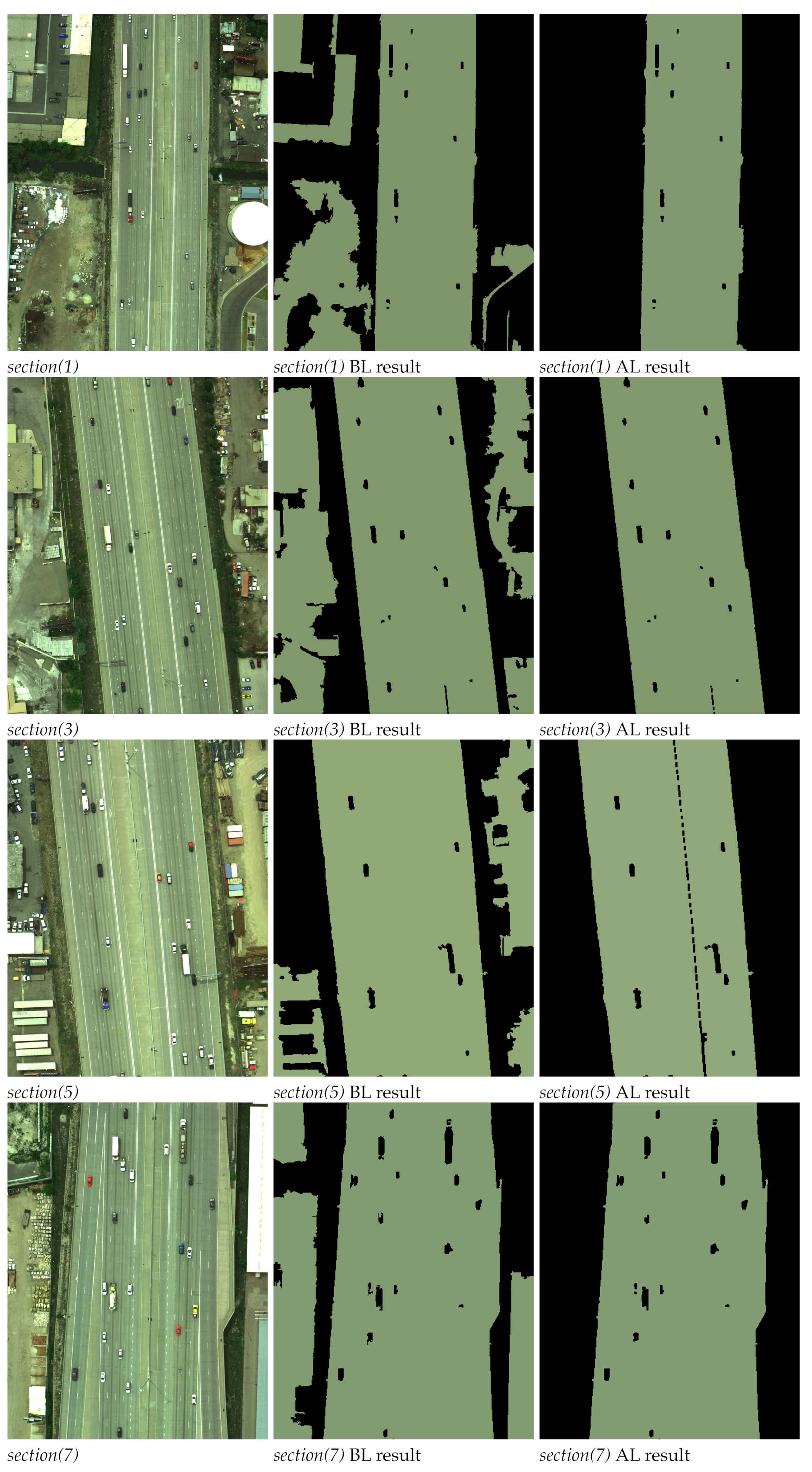
To demonstrate the effectiveness of the last learning step of the road extraction method, we further compared road extraction results with the results without involving learning on 20 sections of airborne color images. Figure 6 compares road extraction results before employing the last learning step and after employing the last learning step for four selected sections, namely, section(1), section(3), section(5), and section(7). The results before learning (BL) clearly showed that buildings, parking lots, and vegetation regions were part of road extraction results since they were similar to the road. The results after learning (AL) showed that with the help of the learning step, the proposed road extraction method effectively identified the road region and removed buildings, parking lots, and vegetation regions that were similar to the road region. These comparison results showed the effectiveness of using the optimization with equality constraints to remove objects that were similar to the road from the extraction results (i.e., to better classify a pixel as road or non-road).

3.2. Traffic Sign Candidate Detection and Classification Results

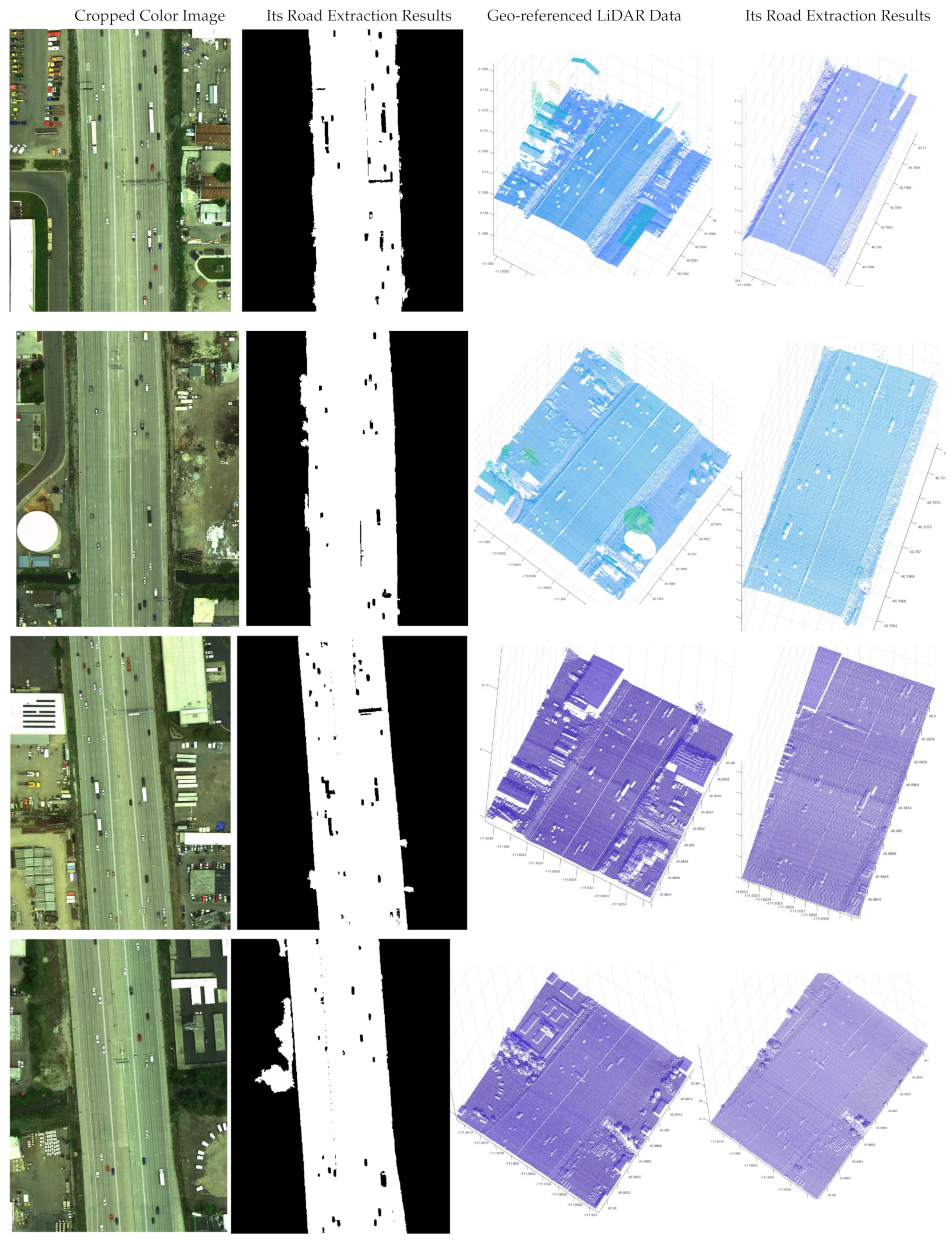
To evaluate the performance of the proposed traffic sign candidate detection and classification method, we conducted extensive experiments on the same 20 sections of the road. Figure 7 presents extracted road regions in both color images and their associated LiDAR data for four selected regions, which were cropped from the sections of the road for better illustration purpose. In each row, we demonstrate the color image of one of four cropped sections of the road and its corresponding road extraction results alongside with its associated geo-referenced LiDAR data and its corresponding road extraction results. It should be mentioned that these four sections contained various objects including the road, buildings, parking lots, vegetation, traffic signs, billboards, and bridges to illustrate the effectiveness of traffic sign detection results. Figure 7 clearly shows that road regions extracted from color images were correctly mapped to the corresponding road regions in the LiDAR data by employing the image to global coordinate projection. Since it is much easier to extract road regions in a color image using complementary features, we utilized road extraction results in color image to quickly find road regions in LiDAR data.

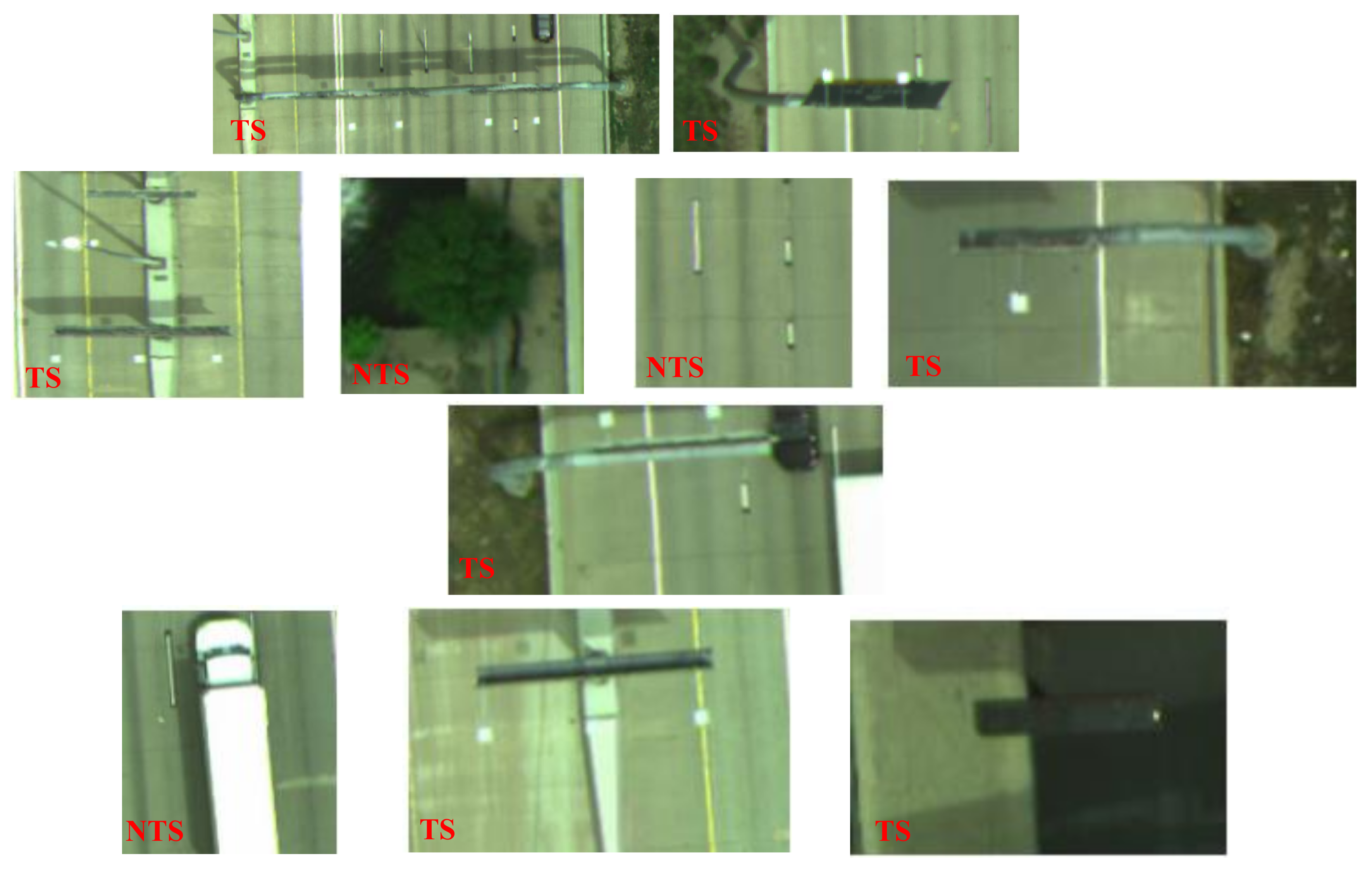
Utilizing a histogram to obtain height statistics, we could quickly remove high elevated objects above the road to find traffic sign candidates in the LiDAR data. Figure 8 demonstrates traffic sign candidates that were extracted from road regions presented in Figure 7, where each row shows extracted traffic sign candidates for each section of the road. These candidates were fed into the sparse classifier optimization model to be classified to a traffic sign class or a non-traffic sign class by empirically setting the parameter p to be 0.6 as shown in Figure 2. We labeled the classification result of each traffic sign candidate at the bottom left of each airborne color image with “TS” indicating a traffic sign and “NTS” indicating a non-traffic sign.

To quantitatively evaluate the proposed traffic sign detection method, we provided its true positives, false negatives, and true negatives on all the 20 sections of the dataset containing 17 traffic signs in total. The proposed method extracted 24 traffic sign candidates by removing high elevated objects above the road in the LiDAR data. The deep-features-based sparse classifier correctly classified 14 out of 24 candidates as traffic signs (true positives), incorrectly classified three out of 24 candidates as non-traffic signs (false negatives), and correctly classified seven out of 24 candidates as non-traffic signs (true negatives). In other words, the proposed method was able to successfully extract 14 out of 17 traffic signs and achieved the detection accuracy of 82.35%. We further provided four evaluation measures including recall (detection rate), precision, $F_1$-measure, and quality in

Table 1. Summary of traffic sign detection results in terms of four measures.

	Precision	Recall	${\mathit{F}}_1$-Measure	Quality
Traffic Sign Class	82.35%	100%	90.32%	82.35%

. These measures were computed as follows:

$$Recall=\frac{\mathrm{True} \mathrm{Positives}}{\mathrm{True} \mathrm{Positives}+\mathrm{False} \mathrm{Positives}}$$

(11)

$$Precision=\frac{\mathrm{True} \mathrm{Positives}}{\mathrm{True} \mathrm{Positives}+\mathrm{False} \mathrm{Negatives}}$$

(12)

$$F_1-\mathit{measure}=2\times \frac{\mathrm{Precision}\times \mathrm{Recall}}{\mathrm{Precision}+\mathrm{Recall}}$$

(13)

$$quality=\frac{\mathrm{True} \mathrm{Positives}}{\mathrm{True} \mathrm{Positives}+\mathrm{False} \mathrm{Positives}+\mathrm{False} \mathrm{Negatives}}$$

(14)

It shows that the proposed method achieved an average precision of 82.35%, a recall of 100%, a $F_1$-measure of 90.32%, and a quality of 82.35%. This performance is attributed to the use of the optimization with equality constraints to more accurately classify a pixel as road or non-road, the use of deep features to more accurately representing the visual data of candidates, and the use of the sparse classifier optimization model to more accurately classify each candidate as traffic sign or non-traffic sign.

3.3. Comparison with Other Methods

Extracting road and detecting traffic signs along the road in one source of the input (i.e., LiDAR data or color images) is not straightforward. For instance, it is challenging to segment 3D LiDAR data and extract road from the segments mainly due to high level of noise. It is also challenging to detect traffic signs due to their low density in the airborne LiDAR data. We implemented the method proposed in [30] to segment the road in LiDAR data and the method proposed in [31] to identify traffic signs along the road in LiDAR data. To this end, we extracted 3D hand-crafted features [30], namely, normal vectors and principal curvatures, to segment road in our airborne LiDAR data. We obtained inaccurate segmentation results, which contained many of the parking lot areas along the road, due to similar normal vectors and curvatures for parking lots and road. We further extracted 3D deep features [31] to segment and classify traffic signs in our airborne LiDAR data. We obtained inaccurate segmentation and classification results since 3D deep features capture a lot of noise in the data. On the other hand, traffic signs appeared with low density in our airborne LiDAR data. As a result, they did not form any recognizable shape and were difficult to be detected as any solid objects. Our experimental results on the airborne LiDAR data showed that seven non-traffic signs were detected as traffic signs. These seven non-traffic signs could be easily filtered out if we fused the complementary information from both color images and LiDAR data.

Similarly, detecting traffic signs in airborne color images is also challenging since the height and shape information of traffic signs is missing in the 2D data. We cannot compare the performance of other methods of detecting traffic signs in color images with ours since they do not process airborne color images, where traffic signs do not exhibit any rectangular shapes.

To the best of our knowledge, there is no research working on registered airborne geo-referenced color images and airborne LiDAR data to detect traffic signs. Therefore, we cannot compare the proposed method with state-of-the-art methods in this regard. In addition, comparing the performance of the proposed method with the performance of previous studies on the same dataset is challenging due to the differences in datasets and the variation of the defined tasks. For instance, one method working well on a high density MLS point cloud collected from a city area may not obtain a good performance on airborne LiDAR data collected from highway and vice versa. This is mainly due to different scan angles of objects, point cloud density, and noise level. Instead, we compared the performance of the proposed method with several traffic sign detection methods that worked with either LiDAR data or color images to demonstrate the effectiveness of the proposed fusion technique. We chose four methods [5,9,10,32], to compare their performance of detecting traffic signs in the LiDAR data with ours. However, this comparison was difficult due to the difference of datasets in terms of the quality, density, and distribution of the point clouds, areas (city vs. highway) where the data were collected from, and the data source (mobile LiDAR vs. airborne LiDAR). In [32], the authors report a recall rate of 65% and a precision rate of 58% for 60 traffic signs. A recall of 60.81% and a precision of 95.74% are reported in [5]. Lehtomäki et al. [9] report a recall of 65.96% and a precision of 93.94%. Javanmardi et al. [10] report a performance of 94.48% and 84.04% in terms of recall and precision, respectively. Our proposed fusion method achieved 100% recall and 82.35% precision. Specifically, it correctly detected 14 out of 17 traffic signs. The proposed method outperformeed [32] in term of precision rate and achieved the highest recall rate among the compared methods.

4. Conclusions

In this paper, we utilize information captured from airborne geo-referenced color images and noisy airborne LiDAR data to fuse the complementary information and accurately detect traffic signs. Our designed method includes three major steps: (1) road extraction, (2) traffic sign candidate detection, and (3) traffic sign classification. Six joint local features are seamlessly incorporated in the aggregation optimization model to accurately identify the road region in color images. Histogram of height information is utilized along the road region in the LiDAR data mapped by the image to global coordinate projection to detect traffic sign candidates. Local deep features are also incorporated in the sparse representation-based optimization model to accurately identify traffic sign candidates in color images mapped by the global to image coordinate projection. Both qualitative and quantitative results show the effectiveness of the proposed method to detect traffic signs. Some of the important findings are summarized as follows:

• Using the complementary information from color images and airborne LiDAR data improves the accuracy of traffic sign detection.
• Extracting road regions is an essential initial step, which significantly reduces the search space for traffic signs to improve the detection efficiency.
• Representing local deep features in a sparse representation-based local-embedded optimization model helps to capture the local structure of traffic signs for more accurate classification.

With the advent of unmanned aerial vehicle (UAV) technology, high-resolution aerial images and LiDAR data will be much more affordable and easily accessible for transportation agencies in the future. Although the current data set was collected with a fixed-wing plane, the methodology developed for the current data set will be readily transferable to any UAV-based data collection platform.

References

1. He, Y.; Song, Z.; Liu, Z. Updating highway asset inventory using airborne LiDAR. Measurement 2017, 104, 132–141. [Google Scholar] [CrossRef]
2. Soheilian, B.; Paparoditis, N.; Vallet, B. Detection and 3D reconstruction of traffic signs from multiple view color images. ISPRS J. Photogramm. Remote Sens. 2013, 77, 1–20. [Google Scholar] [CrossRef]
3. Adam, A.; Ioannidis, C. Automatic road-sign detection and classification based on support Vector machines and HOG descriptors. ISPRS Ann. Photogramm. Remote Sens. Spat. Inf. Sci. 2014, 2. [Google Scholar] [CrossRef] [Green Version]
4. Khalid, S.; Muhammad, N.; Sharif, M. Automatic measurement of the traffic sign with digital segmentation and recognition. IET Intell. Transp. Syst. 2018, 13, 269–279. [Google Scholar] [CrossRef]
5. Pu, S.; Rutzinger, M.; Vosselman, G.; Elberink, S.O. Recognizing basic structures from mobile laser scanning data for road inventory studies. ISPRS J. Photogramm. Remote Sens. 2011, 66, S28–S39. [Google Scholar] [CrossRef]
6. Yokoyama, H.; Date, H.; Kanai, S.; Takeda, H. Detection and classification of pole-like objects from mobile laser scanning data of urban environments. Int. J. CAD/CAM 2013, 13, 31–40. [Google Scholar]
7. Yu, Y.; Li, J.; Guan, H.; Wang, C. Automated extraction of urban road facilities using mobile laser scanning data. IEEE Trans. Intell. Transp. Syst. 2015, 16, 2167–2181. [Google Scholar] [CrossRef]
8. Riveiro, B.; Díaz-Vilariño, L.; Conde-Carnero, B.; Soilán, M.; Arias, P. Automatic segmentation and shape-based classification of retro-reflective traffic signs from mobile LiDAR data. IEEE J. Sel. Top. Appl. Earth Obs. Remote Sens. 2015, 9, 295–303. [Google Scholar] [CrossRef]
9. Lehtomäki, M.; Jaakkola, A.; Hyyppä, J.; Lampinen, J.; Kaartinen, H.; Kukko, A.; Puttonen, E.; Hyyppä, H. Object classification and recognition from mobile laser scanning point clouds in a road environment. IEEE Trans. Geosci. Remote Sens. 2016, 54, 1226–1239. [Google Scholar] [CrossRef] [Green Version]
10. Javanmardi, M.; Song, Z.; Qi, X. Automated traffic sign and light pole detection in mobile LiDAR scanning data. IET Intell. Transp. Syst. 2018, 13, 803–815. [Google Scholar] [CrossRef]
11. Zohrizadeh, F.; Kheirandishfard, M.; Ghasedidizaji, K.; Kamangar, F. Reliability-based local features aggregation for image segmentation. In International Symposium on Visual Computing (ISVC); Springer: Las Vegas, NV, USA, 2016; pp. 193–202. [Google Scholar]
12. Li, Z.; Chen, J. Superpixel segmentation using linear spectral clustering. In Proceedings of the IEEE Conference on Computer Vision and Pattern Recognition, Boston, MA, USA, 7–12 June 2015; pp. 1356–1363. [Google Scholar]
13. Berry, M.W.; Browne, M.; Langville, A.N.; Pauca, V.P.; Plemmons, R.J. Algorithms and applications for approximate nonnegative matrix factorization. Comput. Stat. Data Anal. 2007, 52, 155–173. [Google Scholar] [CrossRef] [Green Version]
14. Boyd, S.; Boyd, S.P.; Vandenberghe, L. Convex Optimization. Cambridge University Press: New York, NY, USA, 2004. [Google Scholar]
15. Javanmardi, M.; Qi, X. Structured group local sparse tracker. IET Image Process. 2019, 13, 1391–1399. [Google Scholar] [CrossRef] [Green Version]
16. Boyd, S.; Parikh, N.; Chu, E.; Peleato, B.; Eckstein, J. Distributed optimization and statistical learning via the alternating direction method of multipliers. Found. Trends Mach. Learn. 2011, 3, 1–122. [Google Scholar] [CrossRef]
17. Chatfield, K.; Simonyan, K.; Vedaldi, A.; Zisserman, A. Return of the devil in the details: Delving deep into convolutional nets. arXiv 2014, arXiv:1405.3531. [Google Scholar]
18. Krizhevsky, A.; Sutskever, I.; Hinton, G.E. Imagenet classification with deep convolutional neural networks. Commun. ACM 2017, 60, 84–90. [Google Scholar] [CrossRef]
19. Hong, S.; Noh, H.; Han, B. Decoupled deep neural network for semi-supervised semantic segmentation. Adv. Neural Inf. Process. Syst. 2015, 28, 1495–1503. [Google Scholar]
20. Simonyan, K.; Zisserman, A. Very deep convolutional networks for large-scale image recognition. arXiv 2014, arXiv:1409.1556. [Google Scholar]
21. Girshick, R.; Donahue, J.; Darrell, T.; Malik, J. Rich feature hierarchies for accurate object detection and semantic segmentation. In Proceedings of the IEEE Conference on Computer Vision and Pattern Recognition, Columbus, OH, USA, 23–28 June 2014; pp. 580–587. [Google Scholar]
22. Ma, C.; Huang, J.B.; Yang, X.; Yang, M.H. Hierarchical convolutional features for visual tracking. In Proceedings of the IEEE International Conference on Computer Vision, Araucano Park, Las Condes, Chile, 7–13 December 2015; pp. 3074–3082. [Google Scholar]
23. Javanmardi, M.; Qi, X. Appearance variation adaptation tracker using adversarial network. Neural Netw. 2020, 129, 334–343. [Google Scholar] [CrossRef]
24. Javanmardi, M.; Farzaneh, A.H.; Qi, X. A Robust Structured Tracker Using Local Deep Features. Electronics 2020, 9, 846. [Google Scholar] [CrossRef]
25. Deng, J.; Dong, W.; Socher, R.; Li, L.J.; Li, K.; Fei-Fei, L. Imagenet: A large-scale hierarchical image database. In Proceedings of the International Conference on Computer Vision and Pattern Recognition (CVPR), Miami, FL, USA, 20–25 June 2009; pp. 248–255. [Google Scholar]
26. Jia, X.; Lu, H.; Yang, M.H. Visual tracking via adaptive structural local sparse appearance model. In Proceedings of the International Conference on Computer Vision and Pattern Recognition (CVPR), Providence, RI, USA, 16–21 June 2012; pp. 1822–1829. [Google Scholar]
27. Dollár, P.; Zitnick, C.L. Structured forests for fast edge detection. In Proceedings of the International Conference on Computer Vision (ICCV), Sydney, Australia, 1–8 December 2013. [Google Scholar]
28. Leordeanu, M.; Sukthankar, R.; Sminchisescu, C. Generalized boundaries from multiple image interpretations. IEEE Trans. Pattern Anal. Mach. Intell. 2014, 36, 1312–1324. [Google Scholar] [CrossRef] [PubMed]
29. Malik, J.; Belongie, S.; Shi, J.; Leung, T. Textons, contours and regions: Cue integration in image segmentation. In Proceedings of the International Conference on Computer Vision (ICCV), Kerkyra, Greece, 20–27 September 1999. [Google Scholar]
30. Rusu, R.B.; Cousins, S. 3D is here: Point Cloud Library (PCL). In Proceedings of the IEEE International Conference on Robotics and Automation (ICRA), Shanghai, China, 9–13 May 2011. [Google Scholar]
31. Qi, C.R.; Su, H.; Mo, K.; Guibas, L.J. Pointnet: Deep learning on point sets for 3d classification and segmentation. In Proceedings of the International Conference on Computer Vision and Pattern Recognition (CVPR), Honolulu, HI, USA, 21–26 July 2017; pp. 652–660. [Google Scholar]
32. Golovinskiy, A.; Kim, V.G.; Funkhouser, T. Shape-based recognition of 3D point clouds in urban environments. In Proceedings of the IEEE 12th International Conference on Computer Vision, Kyoto, Japan, 29 September–2 October 2009; pp. 2154–2161. [Google Scholar]
Figure 1. The overview of the proposed method.
Applsci 11 00309 g001
Figure 2. The overview of the proposed deep-features-based sparse classifier optimization model.
Applsci 11 00309 g002
Figure 3. A sample section of a geo-referenced color image of the dataset.
Applsci 11 00309 g003
Figure 4. Road extraction results for four sections of the road, section(1), section(2), section(3), and section(4).
Applsci 11 00309 g004
Figure 5. Road extraction results for another four sections of the road, section(5), section(6), section(7), and section(8).
Applsci 11 00309 g005
Figure 6. Comparison of road extraction results before and after employing the last learning step for four sections of the road, section(1), section(3), section(5), and section(7).
Applsci 11 00309 g006
Figure 7. Road extraction results in both color images and their associated LiDAR data for four cropped sections.
Applsci 11 00309 g007
Figure 8. Extracted traffic sign candidates and their classification labels for four sections of the road.
Applsci 11 00309 g008