Article

Utilisation of Ensemble Empirical Mode Decomposition in Conjunction with Cyclostationary Technique for Wind Turbine Gearbox Fault Detection

by
Sanaz Roshanmanesh
1,†,‡,
Farzad Hayati
2,‡ and
Mayorkinos Papaelias
1,*,†,‡
1
School of Metallurgy and Materials, University of Birmingham, Birmingham B15 2TT, UK
2
School of Engineering, University of Birmingham, Birmingham B15 2TT, UK
*
Author to whom correspondence should be addressed.
Current address: School of Metallurgy and Materials, University of Birmingham, Birmingham B15 2TT, UK.
These authors contributed equally to this work.
Appl. Sci. 2020, 10(9), 3334; https://doi.org/10.3390/app10093334
Submission received: 26 March 2020 / Revised: 5 May 2020 / Accepted: 8 May 2020 / Published: 11 May 2020
(This article belongs to the Special Issue Wind Power Technologies)

Abstract

:
In this paper the application of cyclostationary signal processing in conjunction with Ensemble Empirical Mode Decomposition (EEMD) technique, on the fault diagnostics of wind turbine gearboxes is investigated and has been highlighted. It is shown that the EEMD technique together with cyclostationary analysis can be used to detect the damage in complex and non-linear systems such as wind turbine gearbox, where the vibration signals are modulated with carrier frequencies and are superimposed. In these situations when multiple faults alongside noisy environment are present together, the faults are not easily detectable by conventional signal processing techniques such as FFT and RMS.

1. Introduction

With the wind energy global installed capacity reaching 651 GW in 2019 [1], effective remote condition monitoring and predictive maintenance strategies for wind turbines are becoming more significant attracting increased attention. Wind turbines are typically expected to have a design lifespan of 20–25 years. However, they rarely meet this target without major overhauls, particularly in their drivetrain [2]. Gearbox faults and failures take considerable time to repair. Hence, they result in major downtime and loss of production capacity leading to increased maintenance costs for wind farm operators [3,4,5,6].
Direct drive wind turbine designs remove the need for a gearbox. However, the power converters of direct drive wind turbines are among the most frequent failing components which cumulatively result in excessive downtime [7,8]. Thus, the failure rate of power electronics in direct drive wind turbines greatly exceeds the failure rate of the gearbox in geared wind turbines [8]. Nonetheless, due to the advantages and disadvantages of each design, technology forecasts suggest that both geared and direct drive wind turbines will continue to be used in the future [9].
Unlike simple gearboxes used in conventional steady-state machinery, the vibration signals recorded from the gearbox of a wind turbine can be contaminated resulting in erroneous interpretation of the data acquired. Wind turbine gearboxes have very complex designs, comprising many different gears and bearings resulting in the vibration of different parts of the gearbox to superimpose in the recorded vibration signal with multiple frequency and amplitude modulations occurring. Hence, it is very challenging to detect a developing fault in its early stages using conventional signal processing techniques such as Fast Fourier Transform or RMS [10]. Moreover, once a fault is detected it is extremely important from a maintenance point of view to evaluate the severity. Identifying a defect alone is not sufficient for a wind farm operator in order to decide if maintenance is required. In addition, if it is deemed that maintenance is required it is very important to identify when it should be carried out without risking loss of production and expensive outages. Gearboxes are rarely available as spare parts and therefore it can take several months before a spare gearbox can become available. Therefore, it is critical for wind farm operators to pinpoint the exact gearbox component affected by the fault and quantify its severity in order to accurately plan maintenance without the risk of loss of production.
The cyclostationary signal processing technique is a very powerful tool for fault detection in rotating machinery. Moreover, it can be utilised to evaluate the severity of developing faults in rolling elements and bearings. However, as it has been suggested by Dong and Chen [11], this technique is not very successful in complex systems when multiple gears and bearings are present.
Here we have investigated the suitability of combining two advanced signal processing techniques for the purpose of fault detection in the gearbox of wind turbines. These techniques are known as Cyclic Spectral Analysis and Ensemble Empirical Mode Decomposition (EEMD), which will be explained in more details in the next section. It should be stressed, that wind turbines operate in variable loading conditions and therefore, the accurate evaluation of the severity of faults is very challenging [12]. Moreover, false indications of non-existent faults are not uncommon when using conventional signal processing techniques.

2. Theory

2.1. Cyclic Spectral Analysis

The concept of cyclostationary signals has been around for almost 40 years [13,14]. In recent years, the theory of cyclostationary signals has been increasingly used in the field of mechanical fault detection. Vibration signals extracted from bearings and rotating machines are non-stationary signals containing some hidden periodicities in their background. To extract the periodicity many signal processing tools are available. The cyclostationary signal analysis technique is one of the most powerful techniques from those currently available [15]. The statistics of cyclostationary signals have periodicity with respect to time [10]. Currently, second-order cyclostationarity which is known as cyclic correlation [10] has an important role in practical application. Despite the strengths of this technique and its popularity in signal processing of rotating machinery, it has not attracted much attention in the field of wind turbine condition monitoring and signal processing. To describe this technique we start with a random process.
In general, a random process will have a time-varying autocorrelation:
R x ( t , τ ) = E x t + τ 2 x * t τ 2
where E { } denotes the mathematical expectation operator, and τ is the time delay. If the autocorrelation is considered periodic with a period of T 0 , the ensemble average can be estimated with a time average as below:
R x ( t , τ ) = lim N n = N N x t + n T 0 + τ 2 x * t + n T 0 τ 2
The autocorrelation function in Equation (1) can be written in form of Fourier series due to its periodicity
R x ( t , τ ) = α R x α ( τ ) e j 2 π α t
where α = m / T 0 and m Z . Combining the above equation with the Equation (2), the Fourier coefficients can be written as below
R x α ( τ ) = lim T 1 T T 2 T 2 x t + τ 2 x * t τ 2 e j 2 π α t d t = x t + τ 2 x * t τ 2 e j 2 π α t t
where R x α ( τ ) is known as cyclic autocorrelation function with α being the cyclic frequency. The symbol represents the time averaging operator. Next, to obtain the cyclic spectrum, the Fourier transform can be applied to the cyclic autocorrelation function with respect to the time delay τ , yielding
S x α ( f ) = R x α ( τ ) e j 2 π f τ d τ
that is known as cyclic spectrum or the spectral correlation function.
In this work the Welch’s averaged periodogram technique has been used, that due to its high computational efficiency is one of the most common estimators for cyclic spectrum [16].
The cyclic coherence that measures the strength of the correlation between spectral components distanced by cyclic frequencies can be calculated using [16]
C x α ( f ) = S x α ( f ) S x 0 ( f + α / 2 ) S x 0 ( f α / 2 )

2.2. Empirical Mode Decomposition

The Empirical Mode Decomposition (EMD) is the fundamental part of a technique known as Hilbert–Huang Transform that is an empirical data analysis technique, developed in late 1990s by Huang et al. [17,18,19]. Unlike other techniques such as Fourier or Wavelet Transforms, that use prior knowledge or fixed basis to decompose the signal, EMD derives its basis adaptively from the data itself and does not rely on any prior knowledge [20]. This technique is based on an assumption that any data is consisting of a set of simple intrinsic modes of oscillations [21].
The EMD decomposition process, decomposes the original signal into a set of signals known as Intrinsic Mode Functions (IMFs). This is accomplished by a novel process known as sifting, which is repeatedly applied to the signal until it converges on criteria that define an IMF [20]. The EMD sifting process extracts the fastest varying component first and continues to the next IMF. The process produces a finite number of IMFs before converging itself.
The extracted IMFs represent simple oscillatory functions with different time-scale. Each IMF by definition will have the same number of extrema and zero-crossings or differ at most by one. Furthermore, the mean value of the envelopes of local maxima and local minima of IMFs are zero at any given point [21]. The technique to calculating the IMFs are briefly explained here but for more details and derivations on the technique one can refer to [17,21].
The first step to calculate the IMF is to find all the local maxima points of the signal and connect them using cubic spline to obtain the upper envelope of the signal. The same procedure is applied to the local minima points to obtain the lower envelope. Next, the mean value of the two envelopes is calculated. The first component of the signal is calculated by subtracting the obtained mean from the original signal
h 1 ( t ) = x ( t ) m 1 ( t )
where x ( t ) is the original signal and m 1 is the calculated mean. If the calculated component h 1 meets the IMF criteria, then it will be the first IMF. However if the calculated component does not meet the requirement of an IMF, the procedure is repeated again by replacing the original signal x ( t ) with h 1 . This cycle is repeated until the calculated component meets the IMF criteria. It is then marked as the first IMF ( c 1 ) and subtracted from the original signal.
x n e w ( t ) = x ( t ) c 1 ( t )
After this step, the original signal x ( t ) is replaced with the new signal x n e w ( t ) and the whole procedure is repeated to calculate the next IMFs. The remaining signal after calculating the last IMF is called the residual signal r ( t ) and can be used to reconstruct the original signal using the calculated IMFs using
x ( t ) = i = 1 n c i ( t ) + r ( t )
where n represent the number of calculated IMFs. This process is summarised in Figure 1.
Although this technique is very effective in decomposing non-linear and non-stationary signals, it suffers from certain problems such as end effect or mode mixing (aliasing) which was noted by Huang himself [19]. One solution to avoid the mode mixing problem is to use a newly proposed technique known as Ensemble EMD (EEMD) [23]. This technique uses noise assisted analysis to solve the problem of mode mixing in the EMD algorithm.
This can be done by adding White Gaussian noise to the signal. Consider adding noise to the proposed signal for M times and each time decomposing the signal using EMD technique. Each new signal can be presented as
x i ( t ) = x ( t ) + w i ( t )
where w i ( t ) represents the i-th added white noise to the original signal x ( t ) and x i ( t ) is the generated noisy signal. Using Equation (9) we can reconstruct the i-th noisy signal as
x i ( t ) = j = 1 n c i j + r i ( t )
where c i j is the j-th calculated IMF of noisy signal x i ( t ) and r i ( t ) is the residual signal. Now we can ensemble the corresponding IMF over noisy signals to obtain the resulting IMFs
c j = 1 M i = 1 M c i j + r ( t )
where M is the total number of times that the white noise was added to the signal. The accuracy of the result obtained using EEMD is highly dependent on the number of ensemble and the amplitude of the added noise ( ε ). Using a well-established statistical rule such as Equation (13), the standard deviation of error ( ε n ) in the final IMFs can be calculated [23].
ε n = ε N

3. Measurement Setup

The evaluation of the proposed technique was done using three different testing setups. Initially, a lightly contaminated signal recorded from a simple rolling element bearing was used to evaluate the performance of the cyclostationary analysis, as well as its combination with EEMD.
Next, a more complex scenario was considered with a signal recorded from an input shaft of a 3-stage gearbox in a mock-up wind turbine. Finally, the data recorded from the gearbox of a real wind turbine, during full load operation, was used to evaluate the performance of the technique. Each of these three setups is detailed below.

3.1. Rolling Element Test Rig

A simple customised test rig shown in Figure 2 was used for bearing test at the University of Birmingham. The test rig consists of an AC motor rotating a shaft via pulley and belt. A controlled load was applied to the rolling element under investigation. The speed of the bearing was monitored using a tachometer. The sensor which was used to record the vibration signal was a high frequency 712F accelerometer by Wilcoxon Corporation with a nominal range of 3 Hz to 25 KHz.

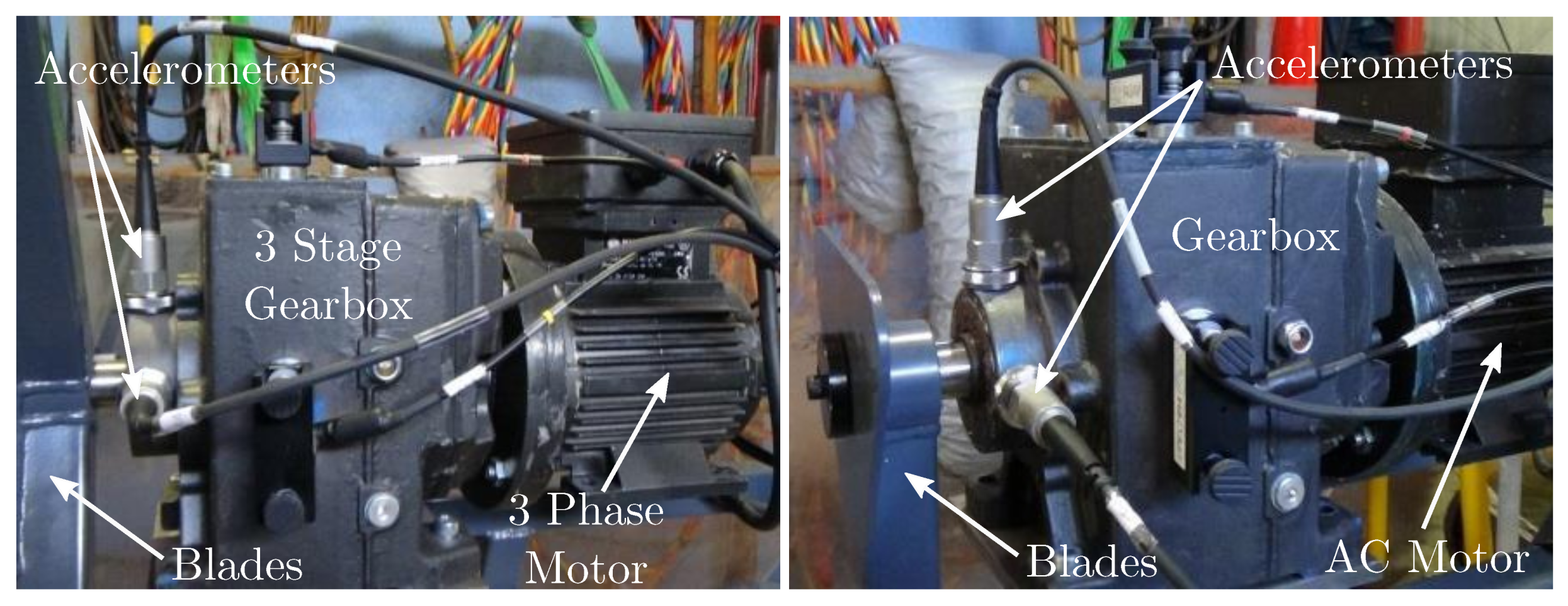
3.2. Tidal Turbine Gearbox Test Rig

The test rig used for these measurements has been developed by TWI Ltd. in the UK and the University of Brunel in an effort to replicate a geared tidal turbine with the ability to be submerged into the water. The test rig consists of a 3-phase 750 Watt AC motor controlled by a Variable Frequency Driver (VFD) capable of running at 1500 rpm, a 3-stage spur and helical parallel gearbox with a ratio of approximately 1:69 and 3 blades at the main shaft turning at approximately 22 rpm. The tidal turbine gearbox test rig setup is shown in Figure 3.
This test rig is instrumented with two accelerometers in X and Y directions mounted on the input shaft of the gearbox (i.e., slow speed shaft) over the bearing to record vibration data of the gear box. The sensors used are AC 150-2C accelerometer by Connection Technology Centre Inc with a nominal range of 1 Hz to 10 kHz.

3.3. Wind Turbine Gearbox

Vibration data were recorded from an operational industrial wind turbine at full load using an INGESYS system manufactured by INGETEAM Service, Spain. The monitored wind turbine had a rated power of 850 kW with a 3-stage planetary gearbox and a ratio of approximately 1:62. The wind turbine was known to be due for maintenance and it had some gear teeth wear and bearing damage at the planetary stage.
The INGESYS monitoring system was installed in an industrial cabinet in the nacelle of the wind turbine. It consists of the power supply, communications and vibration acquisition system. During testing it was connected to the ground data recording unit using fibre optic.
In order to measure vibrations in the drive-train, 8 piezoelectric accelerometers were used. Two of them were specifically selected to measure low vibration frequencies in the main shaft. The two types of the accelerometer sensors that were used are PRE-1010-MS and PRE-1030-MS by IMI Sensors capable of covering the range of 0.5 Hz to 10 kHz and 2 Hz to 10 kHz, respectively. These sensors were installed on both radial and axial directions on the main shaft, planetary stage, high speed shaft and the generator. Some of the accelerometers installed on the wind turbine gearbox are shown in Figure 4.

4. Results and Discussions

4.1. Rolling Element Analysis

Two identical tapered roller bearing with different induced faults were used in this setup. The first roller bearing was damaged on its both outer races and the second roller bearing was scuffed on the roller surface as shown in Figure 5. Each scuffed roller was placed in one of the bearing races. The recorded signal from these bearings was also expected to be contaminated with some noise originating from the AC motor, pulley, belt and other nearby bearings used in the test-rig itself. The characteristic frequencies of the rolling element used for the experiments using the customised test rig at the University of Birmingham are summarised in Table 1.
In each case, it is expected to observe the presence of the bearing characteristic frequency corresponding to the induced fault. In the case of the first bearing, the Ball Pass Frequency of Outer race (BPFO) is expected to be dominant. For the second bearing, the Ball Spin Frequency (BSF) that indicates the frequency of which the roller is turning can be used to identify the fault. However, as the rollers turn, the scuffed area will hit both the inner and outer race in each revolution. Thus, the observed defect frequency is expected to be twice the BSF frequency.
The Cyclic Spectral Coherence was calculated over 4 s of the vibration data. As it can be seen in Figure 6, the BPFO frequency is clearly visible. Alongside the BPFO frequency, some modulations at the BSF frequency are also present which indicate damage in the rolling elements. This was confirmed by inspection of the rollers after testing. The outer race damage and heavy load on the bearing caused the surface of the rollers to degrade. However, the degradation was not significant.
Similar to the first bearing, 4 s of vibration data were recorded from the second bearing and then used to calculate the Cyclic Spectral Coherence as shown in Figure 7.
As it was mentioned earlier, the fault frequency (2 × BSF) was observed in the Cyclic Spectral Coherence. However, unlike the first bearing frequency, it was more spread across the frequency spectrum. This could have been caused due to two damaged rollers or slight change in the bearing speed during the test arising from the load imposed.
As it can be seen in Figure 7, the fundamental train frequency (4.4 Hz) is also very dominant. This was assumed to be due to the interaction between the damaged roller and the cage. However, after inspection, it was found that one of the damaged rollers led to fracture of the cage of the second bearing.

4.2. Simplified Gearbox Analysis

A simple gearbox operating at steady-state was studied with imbalance caused in the rotor i.e., slow shaft, and the high speed shaft rotating at 750 rpm. The characteristic frequencies of the gearbox are summarised in Table 2.
The Cyclic Spectral Coherence was calculated using 4 s vibration signals. The calculated results are presented in Figure 8. As the induced fault was imbalance, modulations and cyclic behaviour at the gear-mesh (GM) frequency of the first stage of the gearbox (10.5 Hz) were caused.
As it can be seen in Figure 8a, the result from the analysis of the original raw signal is less clear in comparison with the bearing test. For comparison purposes, the analysis was also applied to the de-noised signal using the Wavelet de-noising technique. This was carried out using Daubechies-3 wavelet. However, de-noising the signal worsened the Cyclic Spectral Coherence result as it is shown in Figure 8b.
Using the EEMD technique, the signal was decomposed into 8 IMFs and the Cyclic Spectral Coherence of each IMF was calculated. The result of the first two IMFs is presented in Figure 8c,d respectively. As it can be seen, the result is slightly less contaminated compared with the raw and de-noised signal. However, more interestingly, in Figure 8e,f which shows the result on the 6th and 8th IMFs two other frequencies are visible. These frequencies are the first stage GAPF frequency (5.3 Hz) and the second stage rotational frequency (3.5 Hz).
The presence of both first stage gear mesh and GAPF cyclic behaviour clearly indicates the imbalance applied to the first stage. The existence of the second stage rotational frequency could as well indicate the imbalance. Nonetheless, it can also show the normal vibration contaminating the signal.

4.3. Wind Turbine Gearbox Analysis

The studied gearbox in this part contained 11 different types of bearings. Including the corresponding frequencies of the gears, more than 50 different frequencies of interest were available to analyse. In the present study only the result corresponding to the planetary stage of the gearbox and its bearing defect are shown.
The vibration signal used to analyse the bearing defect at the planetary stage was obtained from the Radial sensor placed at the planetary stage of the gearbox.
The damaged bearing was a cylindrical roller bearing with its characteristic frequencies listed in Table 3. Given the wind turbine working at full rated load, the planets were turning at around 1.07 Hz. The other frequency of interest in the planetary stage fault is the gear-mesh of the planets which was calculated to be 140.84 Hz. The next nearest calculated frequencies to this frequency were 99.1 Hz and 192.5 Hz belonging to the intermediate and high-speed shaft bearings.
As it can be seen in the Figure 9a,b, the gear-mesh of the planets (140.8 Hz) are present in both spectra, indicating possible damage in the planetary gear. It is also evident that the cyclic spectral coherence of the first IMF of the signal is considerably less contaminated with noise originating from other gears.
Similarly in the Figure 9c,d, the Ball Passing Frequency of Inner race (BPFI) at 8.8 Hz is distinctly visible. The other closest present frequencies to this frequency are 7 Hz and 9.5 Hz corresponding to the sun gear defect and carrier bearing frequencies. Again, similar to the gear mesh analysis the cyclostationary analysis on the first IMF of the signal shown in Figure 9d shows less artefacts related to the other gears.
For comparison purposes, the same signal recorded from the planetary stage was also analysed using FFT, Hilbert transform and Cepstrum that are commonly used in condition monitoring and fault detection. As it can be seen in Figure 10a,b the gear-mesh frequency is not detectable in the applied Cepstrum, FFT or Hilbert analysis while the cyclic spectral coherence enhanced with EEMD preconditioning was able to detect it. Similarly, Figure 10c,d show the same analysis applied to the signal to detect BPFI frequency. Similar to the gear mesh analysis, the BPFI frequency was not detected using either Cepstrum or FFT analysis. Although, the Hilbert transform analysis shows some peaks around the BPFI frequency, the amplitude of the peaks are not very significant which can lead to underestimation of the severity. Again, using the cyclic spectral coherence with EEMD the BPFI frequency was detected clearly reducing the likelihood of underestimation of the severity of the defect.

5. Conclusions

The rapid growth in the use of wind turbines combined with their operation under severe loading conditions has increased the need for efficient condition monitoring technologies. Early fault detection is important for wind farm operators in order to improve predictive maintenance strategies, reduce unexpected downtime and associated repair costs. Continuously variable operation of the wind turbines and complexity of the multi-stage gearboxes employed makes it very challenging to detect developing faults particularly during the early stages of evolution.
The cyclostationary technique has been proven to be a very effective tool to detect faults in rotating machinery. However as the complexity of the system increases, the performance of this technique degrades and the results get contaminated with various artefacts coming from different parts of the system.
In this paper the Ensemble Empirical Mode Decomposition technique was used to precondition the vibration signal prior to perform the cyclostationary technique. It has been shown that this can improve the performance of the cyclostationary technique and reduce the contamination in the resulting analysed signals.
The Ensemble Empirical Mode Decomposition technique is a very powerful method that has not been fully explored in the field of wind turbine condition monitoring. The present study has shown the potential of this technique to be employed in conjunction with other techniques to enhance the overall performance of various signal processing techniques in wind turbine gearbox condition monitoring. The ability of this technique to separate the signal into its intrinsic modes, as it was demonstrated in this paper, opens new opportunities in advanced signal processing that are yet to be explored in more depth.

Author Contributions

S.R. and F.H. developed and carried out the signal processing methodology employed in the study, M.P. organised and led the experiments carried out. All authors have read and agreed to the published version of the manuscript.

Funding

This research was partially funded by European Union’s Seventh Framework grant number 322430.

Acknowledgments

The authors would like to thank the several industrial partners anonymised in this paper due to confidentiality reasons for their support. The authors would also like to thank TWI Limited, Brunel University and INGETEAM service for their assistance with some of the tests. The authors are indebted to the EC for partially funding this research as part of the OPTIMUS FP7 industrial collaborative project.

Conflicts of Interest

The authors declare no conflict of interest.

Abbreviations

The following abbreviations are used in this manuscript:
BPFIBall Pass Frequency of Inner race
BPFOBall Pass Frequency of Outer race
BSFBall Spin Frequency
EEMDEnsemble Empirical Mode Decomposition
EMDEmpirical Mode Decomposition
FTFFundamental Train Frequency
GMGear-mesh
GAPFGear Assembly Phase Frequency
IMFIntrinsic Mode Function

References

  1. Global Wind Statistics. Global Wind Report 2019. Available online: https://gwec.net/global-wind-report-2019 (accessed on 15 April 2020).
  2. Barszcz, T. Vibration-Based Condition Monitoring of Wind Turbines, 1st ed.; Springer: Cham, Switzerland, 2019. [Google Scholar] [CrossRef]
  3. Pérez, J.M.P.; Márquez, F.P.G.; Tobias, A.; Papaelias, M. Wind turbine reliability analysis. Renew. Sustain. Energy Rev. 2013, 23, 463–472. [Google Scholar] [CrossRef]
  4. Márquez, F.P.G.; Tobias, A.M.; Pérez, J.M.P.; Papaelias, M. Condition monitoring of wind turbines: Techniques and methods. Renew. Energy 2012, 46, 169–178. [Google Scholar] [CrossRef]
  5. Zhou, J.; Roshanmanesh, S.; Hayati, F.; Junior, V.J.; Wang, T.; Hajiabady, S.; Li, X.; Basoalto, H.; Dong, H.; Papaelias, M. Improving the reliability of industrial multi-MW wind turbines. Insight-Non Test. Cond. Monit. 2017, 59, 189–195. [Google Scholar] [CrossRef] [Green Version]
  6. Ferrando Chacon, J.L.; Andicoberry, E.A.; Kappatos, V.; Papaelias, M.; Selcuk, C.; Gan, T.H. An experimental study on the applicability of acoustic emission for wind turbine gearbox health diagnosis. J. Low Freq. Noise Vib. Act. Control 2016, 35, 64–76. [Google Scholar] [CrossRef]
  7. Fischer, K.; Pelka, K.; Puls, S.; Poech, M.H.; Mertens, A.; Bartschat, A.; Tegtmeier, B.; Broer, C.; Wenske, J. Exploring the Causes of Power-Converter Failure in Wind Turbines based on Comprehensive Field-Data and Damage Analysis. Energies 2019, 12, 593. [Google Scholar] [CrossRef] [Green Version]
  8. Junior, V.J.; Zhou, J.; Roshanmanesh, S.; Hayati, F.; Hajiabady, S.; Li, X.; Dong, H.; Papaelias, M. Evaluation of damage mechanics of industrial wind turbine gearboxes. Insight-Non Test. Cond. Monit. 2017, 59, 410–414. [Google Scholar] [CrossRef] [Green Version]
  9. Van de Kaa, G.; van Ek, M.; Kamp, L.M.; Rezaei, J. Wind turbine technology battles: Gearbox versus direct drive-opening up the black box of technology characteristics. Technol. Forecast. Soc. Chang. 2020, 153, 119933. [Google Scholar] [CrossRef]
  10. Feng, Z.; Chu, F. Cyclostationary Analysis for Gearbox and Bearing Fault Diagnosis. Shock Vib. 2015, 2015. [Google Scholar] [CrossRef] [Green Version]
  11. Dong, G.; Chen, J. Investigation into various techniques of cyclic spectral analysis for rolling element bearing diagnosis under influence of gear vibrations. J. Phys. Conf. Ser. 2012, 364, 012039. [Google Scholar] [CrossRef]
  12. Romero, A.; Lage, Y.; Soua, S.; Wang, B.; Gan, T.H. Vestas V90-3MW wind turbine gearbox health assessment using a vibration-based condition monitoring system. Shock Vib. 2016, 2016, 6423587. [Google Scholar] [CrossRef] [Green Version]
  13. Gardner, W.A. (Ed.) An Introduction to Cyclostationary Signals. In Cyclostationarity in Communication and Signal Processing; IEEE Press: New York, NY, USA, 1994; Chapter 1; pp. 1–90. [Google Scholar]
  14. Giannakis, G.B. Cyclostationary Signal Analysis. In The Digital Signal Processing Handbook; Madisetti, V.K., Williams, D.B., Eds.; IEEE Press: New York, NY, USA, 1997; Chapter 17. [Google Scholar]
  15. Ishak, G.; Raad, A.; Antoni, J. Analysis of Vibration Signals Using Cyclostationary Indicators; Institute of Technology of Chartres: Chartres, France, 2013. [Google Scholar]
  16. Antoni, J. Cyclic spectral analysis in practice. Mech. Syst. Signal Process. 2007, 21, 597–630. [Google Scholar] [CrossRef]
  17. Huang, N.E.; Long, S.R.; Shen, Z. The Mechanism for Frequency Downshift in Nonlinear Wave Evolution. In Advances in Applied Mechanics; Academic Press: London, UK, 1996; Volume 32, pp. 59–117. [Google Scholar] [CrossRef] [Green Version]
  18. Huang, N.E.; Shen, Z.; Long, S.R.; Wu, M.C.; Shih, H.H.; Zheng, Q.; Yen, N.C.; Tung, C.C.; Liu, H.H. The empirical mode decomposition and the Hilbert spectrum for nonlinear and non-stationary time series analysis. Proc. R. Soc. Lond. A Math. Phys. Eng. Sci. 1998, 454, 903–995. [Google Scholar] [CrossRef]
  19. Huang, N.E.; Shen, Z.; Long, S.R. A New View of Nonlinear Water Waves: The Hilbert Spectrum. Annu. Rev. Fluid Mech. 1999, 31, 417–457. [Google Scholar] [CrossRef] [Green Version]
  20. Kizhner, S.; Blank, K.; Flatley, T.; Huang, N.E.; Patrick, D.; Hestnes, P. On the Hilbert-Huang Transform Theoretical Developments. 2005. Available online: https://ntrs.nasa.gov/search.jsp?R=20050210067 (accessed on 20 April 2018).
  21. Huang, N.E. Introduction to the Hilbert-huang Transform and Its Related Mathematical Problems. In Hilbert-Huang Transform and Its Applications, 2nd ed.; Huang, N.E., Shen, S.S.P., Eds.; World Scientific: Singapore, 2014; Chapter 1; pp. 1–26. [Google Scholar] [CrossRef]
  22. Lei, Y.; Lin, J.; He, Z.; Zuo, M.J. A review on empirical mode decomposition in fault diagnosis of rotating machinery. Mech. Syst. Signal Process. 2013, 35, 108–126. [Google Scholar] [CrossRef]
  23. Wu, Z.; Huang, N.E. Ensemble Empirical Mode Decomposition: A Noise-Assisted Data Analysis Method. Adv. Adapt. Data Anal. 2009, 1, 1–41. [Google Scholar] [CrossRef]
Figure 1. The procedure to obtain Intrinsic Mode Functions (IMFs) using Empirical Mode Decomposition (EMD) technique, adapted from [22]. Refer to the text for more details.
Applsci 10 03334 g001
Figure 2. Test-rig used to measure the vibration of rolling elements. The figure on the left showing the complete setup and the image on the right is zoomed in on the rolling element under the test.
Applsci 10 03334 g002
Figure 3. The test setup used to measure the vibration of the simple gearbox. On the left the system with 3 blades is visible and on the right a different setup with a single blade is shown.
Applsci 10 03334 g003
Figure 4. The radial vibration sensor installed near the planetary gear on the left and both axial and radial vibration sensors installed on the generator drive end on the right.
Applsci 10 03334 g004
Figure 5. The induced scuffing on the bearing outer race (left) and the roller (right).
Applsci 10 03334 g005
Figure 6. Cyclic Spectral Coherence of the first bearing; top figure shows the BPFO frequency (92.4 Hz) and the BSF (~38 Hz) modulation and the bottom figure shows a slice of the top figure at 7.5 kHz.
Applsci 10 03334 g006
Figure 7. Cyclic Spectral Coherence of the second bearing with roller defect; top figure shows the 2 × BSF frequency (80.0 Hz) and the FTF (4.4 Hz) frequency and the bottom figure is the integration of the top figure along frequency axis.
Applsci 10 03334 g007
Figure 8. Cyclic Spectral Coherence of unbalanced condition. From left to right the top row shows the original signal and filtered signal using Wavelet Daubechies-3 (db3) filter. The middle row is the first and second IMFs and the bottom row is 6th and 8th IMFs.
Applsci 10 03334 g008
Figure 9. Cyclic Spectral Coherence of vibration signal recorded from planetary gearbox of wind turbine. From left to right the top row shows analysis on the original signal and its first IMF showing the gear-mesh of the planets. Similarly, the bottom row is the analysis of the same signal (down sampled) and its first IMF showing the BPFI of the bearing of the planet.
Applsci 10 03334 g009
Figure 10. Conventional techniques applied to vibration signal recorded from planetary gearbox of wind turbine with bearing and gear defect. (a) The Cepstral analysis on the original signal with red dashed line on 7.1 ms representing the gear-mesh of the planets at 140.8 Hz. (b) The Hanning windowed single sided FFT amplitude of both original signal and its Hilbert transform with the red dashed line on 140.8 Hz corresponding to the plants gear-mesh. (c) Same as (a) with the red dashed line showing BPFI of the bearing of planets at 114 ms or 8.8 Hz. (d) Same as (b) with the red dashed line showing BPFI of the bearing of planets at 8.8 Hz.
Applsci 10 03334 g010
Table 1. Summary of the characteristic frequencies of the rolling element used for the experiment. Here, FTF stands for Fundamental Train Frequency, BPFO and BPFI are Ball Pass Frequency of Outer and Inner race respectively; and BSF is Ball Spin Frequency.
SpeedCharacteristic Frequency (Hz)
PRMHzFTFBPFOBPFIBSF
600104.492.3117.740.0
Table 2. The characteristic frequencies of the used gearbox at 740 rpm speed. Here the GAPF stands for Gear Assembly Phase Frequency.
FeatureFrequency (Hz)
Output Shaft12.5
3rd Stage Gear-mesh337.5
Interim Shaft3.55
2nd Stage Gear-mesh35.5
Slow Shaft0.83
1st Stage Gear-mesh11.6
1st GAPF5.8
Input Shaft0.18
Table 3. The unit characteristic frequencies and the operation characteristic frequencies of the bearing used for the planets in the monitored gearbox.
SpeedCharacteristic Frequency (Hz)
PRMHzFTFBPFOBPFIBSF
601.000.4055.6768.3232.550
641.070.4336.0578.8812.721

