A Coordination Space Model for Assemblability Analysis and Optimization during Measurement-Assisted Large-Scale Assembly

Featured Application

For assembly incoordination caused by excessive assembly deviations, the proposed method can predict the assemblability and solve the assembly features that need accuracy compensation, to improve the assembly efficiency.

Abstract

The assembly process is sometimes blocked due to excessive dimension deviations during large-scale assembly. It is inefficient to improve the assembly quality by trial assembly, inspection, and accuracy compensation in the case of excessive deviations. Therefore, assemblability prediction by analyzing the measurement data, assembly accuracy requirements, and the pose of parts is an effective way to discover the assembly deviations in advance for measurement-assisted assembly. In this paper, a coordination space model is constructed based on a small displacement torsor and assembly accuracy requirements. An assemblability analysis method is proposed to check whether the assembly can be executed directly. Aiming at the incoordination problem, an assemblability optimization method based on the union coordination space is proposed. Finally, taking the space manipulator assembly as an example, the result shows that the proposed method can improve assemblability with a better assembly quality and less workload compared to the least-squares method.

1. Introduction

Large-scale mechanical products like ships, automobiles, aircrafts, etc. are complex in structure, large in size, and accurate in assembly quality. The assembly workload of the manufacturing process is heavy [1]. These products often need accuracy compensation in the assembly process because of the excessive assembly deviations, which lead to inefficiency. The assembly deviations might be caused by the eventual poor machining quality of parts, or excessive tolerances set by designers. Thus, the trial assembly is often used to detect the assembly deviations in advance, and the parts are then separated to make an accuracy compensation on the bad dimensions. The assembly process takes a long time by the following steps: Trial assembly, measurement of deviations, separation of parts, and re-trial assembly. Therefore, an assemblability analysis and optimization method based on the measurement data is necessary to predict the assembly deviation and make the accuracy compensation in advance.

With the development of measurement-assisted assembly (MAA) [2], measurement technology has become a bridge between the real world and the digital world. Marguet et al. [3] introduced a MAA application in an airbus assembly line. The least-squares method was used to calculate the optimal pose. Chen et al. [4] proposed a weighted SVD algorithm to obtain the optimal pose of components, which improved the accuracy of pose evaluation. Li et al. [5] proposed a coaxial alignment method using distributed monocular vision. The iterative reweighted particle swarm optimization method was constructed to improve the measurement ability of complicated wearing holes. Wang et al. [6] calculated the assembly clearance of a wing-fuselage assembly based on the optimal pose. The above methods mainly consider the measurement and calculation of the assembly pose, and then realize alignment through pose adjustment tooling. The assembly will be difficult if the quality of the parts is poor.

Assemblability prediction is the first step to judge whether the assembly is qualified in the measurement-assisted assembly. Sukhan et al. [7] evaluated the assemblability based on tolerance propagation. Sanderson et al. [8] assessed the assemblability by the maximum likelihood problem, which was solved by the Kalman filter algorithm. The traditional assemblability evaluation methods are mainly used to find the assembly problem in the design phase, but not in the assembly phase. Cui and Du [9] proposed the concept of pose feasible space to assess the assembly coordination. Yuan et al. [10] proposed an assembly quality assessment method based on weighted geometric constraints to calculate the optimal pose. Wu et al. [11] proposed a constraint coordination index to assess the assembly quality. Ma et al. [12] developed the assembly precision pre-analysis technique in the simulation of virtual assembly. Du et al. [13] proposed a pose decoupling model of the axis tolerance feature to decouple the analysis of any pose within the tolerance domain.

The accuracy compensation methods are used to improve assemblability. The digital compensation method has become a research highlight to improve the assemblability. Davis et al. [14] put forward the method of measuring the assembly clearance and realizing the digital manufacturing of the accuracy compensation gasket. Fabian et al. [15] introduced a shimming method by 3D printing technology, and the assembly clearance was measured by optical measurement. Wang et al. [16] provided a shimming method based on scanned data for a wing box assembly involving non-uniform gaps. In addition, finite element analysis was taken to improve the shimming scheme. Those methods, however, need to be assembled first, followed by measurement of the deviations to be compensated, resulting in a lower efficiency.

Some scholars proposed predictive shimming and predictive fettling methods to improve the assembly efficiency and quality [17]. Cui et al. [18] proposed the oriented points group to calculate the deviation of multiple shaft-and-holes, and the gap was shimmed. Yang et al. [19] analyzed the deviation from the measured point cloud to the model to improve skin finishing. Yu et al. [20] employed a virtual assembly and repair analysis method based on both the geometric design model and object scanning model. Manohar et al. [21] proposed an alternative strategy for predictive shimming, based on machine learning and sparse sensing to first learn gap distributions from historical data. Lei et al. [22] presented an automated and in situ alignment approach with the assistance of computer numerical controlled (CNC) positioners and laser trackers to reduce the finish machining workload. The above studies are aimed at specific cases.

The accuracy compensation method is usually applied after assembly. Then, the assembly sometimes needs be separated, which leads to low efficiency. In this paper, an assemblability analysis and optimization method based on the coordination space model is constructed during measurement-assisted large-scale assembly. In Section 2, the coordination space model based on the small displacement torsor is constructed. In Section 3, the assemblability analysis based on the coordination space model is proposed. In addition, the uncoordinated case is further analyzed. In Section 4, the assemblability optimization method based on the union coordination space is proposed for the uncoordinated case. In Section 5, the space manipulator assembly is taken as an example to verify the proposed method. The result shows that the proposed method can optimize the assemblability with less workload and better assembly quality compared to the least-squares method.

2. Coordination Space Model Based on Small Displacement Torsor

Assemblability refers to the ability of parts to satisfy the assembly accuracy requirements in terms of dimensions, which can be expressed by coordination accuracy. Traditionally, coordination accuracy [23] is the difference in the manufacturing dimensions. Figure 1 shows the coordination accuracy of a keyway assembly.

The coordination accuracy is

$${\nabla }_{AB}={∆}_1+{∆}_2=L_A-L_B,$$

(1)

It can be seen that the coordination accuracy is the amount of the allowance on a certain dimension. In this way, the assembly coordination of a single dimension is well presented by coordination accuracy such as angle, length, etc. However, it is not suitable for complicated assembly. Therefore, the concept should be extended to pose allowance space and the space can be predicted by digital measurement data during large-scale assembly. This space is named the assembly coordination space, which is the ability of pose variation under the condition of assembly accuracy requirements, as Figure 2 shows.

The parts of the assembly are divided into the reference part and the align part. The reference part is the fixed part during assembly and the align part will move to the target pose by the pose adjustment tooling. Assume that the primary measurement data of the two parts are

$$\{\begin{array}{c}{\mathit{P}}^R=\left[{\mathit{p}}_1^R {\mathit{p}}_2^R\dots {\mathit{p}}_n^R\right]\\ {\mathit{P}}^A=\left[{\mathit{p}}_1^A {\mathit{p}}_2^A\dots {\mathit{p}}_n^A\right]\end{array},$$

(2)

where ${\mathit{P}}^R$ and ${\mathit{P}}^A$ are the point sets of the reference part and align part, separately, where ${\mathit{p}}_1^R$, etc. and ${\mathit{p}}_1^A$, etc. are the points of the sets ${\mathit{P}}^R$ and ${\mathit{P}}^A$, respectively. The two parts are separated first. According to the least-squares method, the optimal assembly pose can be calculated by

$$\{\begin{array}{c}{\mathit{P}}^R\approx \mathit{R}{\mathit{P}}^A+\mathit{T}\\ e=\min \left\{{\sum }_{i=1}^n\Vert \mathit{R}{\mathit{p}}_1^A+\mathit{T}-{\mathit{P}}^R{\Vert }^2\right\}\end{array},$$

(3)

where $\mathit{R}$ is the rotation matrix, $\mathit{T}$ is the movement matrix, and $e$ is the minimum residual sum of squares. The singular value decomposition method [24] is taken to calculate the parameter $\mathit{R}$ and $\mathit{T}$. Then, the optimal pose of the align part based on the least-squares method is

$${\mathit{\omega }}_0=\left[\begin{array}{cc}\mathit{R}& \mathit{T}\\ 0& 1\end{array}\right],$$

(4)

The assembly deviation can be predicted by the pose ${\mathit{\omega }}_0$ of the align part. The key assembly characteristics (KAC) [25] are the important geometric structures that have key influences on assembly quality. They are described by measurement data and some dimensions that are not necessary to be measured.

$$\mathit{K}=\left\{\mathit{P},\mathit{G}\right\},$$

(5)

where $\mathit{K}$ is the parameters of a KAC, $\mathit{P}$ is the measurement data, $\mathit{G}$ is the dimensions that are not necessary to be measured. The KACs have an irregular distribution in space during large-scale assembly. As shown in Figure 3, the wing-fuselage assembly is completed by 4 pairs of joints. There are four assembly accuracy requirements on each pair of joints: Two on coaxialities and two on clearances.

The KACs are restrained by assembly accuracy requirements. The assembly accuracy is described as

$$T_j^i=f_j^i\left({\mathit{K}}_i^R,{\mathit{K}}_i^A\right),$$

(6)

where ${\mathit{K}}_i^R$ is the parameters of the ith KAC on the reference part (fuselage), ${\mathit{K}}_i^A$ is the parameters of the ith KAC on the align part (wing), $T_j^i$ is the jth assembly accuracy of the ith KAC, and $f_j^i$ is the mapping from parameters to the assembly accuracy. The assembly accuracy should meet the requirements of assembly accuracy, which is formulated in Equation (7)

$$T_j^i\in \left[T_j^{i-min},T_j^{i-max}\right],$$

(7)

where $T_j^{i-min}$ and $T_j^{i-max}$ are the ranges of $T_j^i$. Substitute Equation (6) into Equation (7):

$$f_j^i\left({\mathit{K}}_i^R,{\mathit{K}}_i^A\right)\in \left[T_j^{i-min},T_j^{i-max}\right],$$

(8)

For the m assembly accuracy requirements on n KACs of the assembly, the constraint equations can be expressed as

$$\forall f_j^i\left({\mathit{K}}_i^R,{\mathit{K}}_i^A\right)\in \left[T_j^{i-min},T_j^{i-max}\right],i\in \left[1,n\right],j\in \left[1,j_i\right],$$

(9)

where $j_i$ is the assembly accuracy requirement number of the ith KAC, $m={\sum }_{i=1}^n{j}_i$. When all KACs satisfy their assembly accuracy requirements, the pose is a valid pose to be aligned.

As shown in Figure 4, the valid pose may not be the only one that satisfies all assembly accuracy requirements. Therefore, the adjacent poses of the primary pose shown in Figure 4a can be analyzed. A small displacement torsor (SDT) [26] represents a tiny rigid body’s pose variation. It is described as

$${\mathit{\omega }}_{\mathsf{\Delta }}=\left(x_{\mathsf{\Delta }},y_{\mathsf{\Delta }},z_{\mathsf{\Delta }},{\alpha }_{\mathsf{\Delta }},{\beta }_{\mathsf{\Delta }},{\gamma }_{\mathsf{\Delta }}\right),$$

(10)

The homogeneous transformation matrix of an SDT is

$${\mathit{\omega }}_{\mathsf{\Delta }}^H=\left[\begin{array}{cccc}\mathit{C}{\gamma }_{\mathsf{\Delta }}\mathit{C}{\beta }_{\mathsf{\Delta }}& -\mathit{S}{\gamma }_{\mathsf{\Delta }}\mathit{C}{\beta }_{\mathsf{\Delta }}& \mathit{S}{\beta }_{\mathsf{\Delta }}& x_{\mathsf{\Delta }}\\ \mathit{S}{\gamma }_{\mathsf{\Delta }}\mathit{C}{\alpha }_{\mathsf{\Delta }}+\mathit{C}{\gamma }_{\mathsf{\Delta }}\mathit{S}{\beta }_{\mathsf{\Delta }}\mathit{S}{\alpha }_{\mathsf{\Delta }}& \mathit{C}{\gamma }_{\mathsf{\Delta }}\mathit{C}{\alpha }_{\mathsf{\Delta }}-\mathit{S}{\gamma }_{\mathsf{\Delta }}\mathit{S}{\beta }_{\mathsf{\Delta }}\mathit{S}{\alpha }_{\mathsf{\Delta }}& -\mathit{C}{\beta }_{\mathsf{\Delta }}\mathit{S}{\alpha }_{\mathsf{\Delta }}& y_{\mathsf{\Delta }}\\ \mathit{S}{\gamma }_{\mathsf{\Delta }}\mathit{S}{\alpha }_{\mathsf{\Delta }}-\mathit{C}{\gamma }_{\mathsf{\Delta }}\mathit{S}{\beta }_{\mathsf{\Delta }}\mathit{C}{\alpha }_{\mathsf{\Delta }}& \mathit{C}{\gamma }_{\mathsf{\Delta }}\mathit{S}{\alpha }_{\mathsf{\Delta }}+\mathit{S}{\gamma }_{\mathsf{\Delta }}\mathit{S}{\beta }_{\mathsf{\Delta }}\mathit{C}{\alpha }_{\mathsf{\Delta }}& \mathit{C}{\beta }_{\mathsf{\Delta }}\mathit{C}{\alpha }_{\mathsf{\Delta }}& z_{\mathsf{\Delta }}\\ 0& 0& 0& 1\end{array}\right]\approx \left[\begin{array}{cccc}1& -{\gamma }_{\mathsf{\Delta }}& {\beta }_{\mathsf{\Delta }}& x_{\mathsf{\Delta }}\\ {\gamma }_{\mathsf{\Delta }}& 1& -{\alpha }_{\mathsf{\Delta }}& y_{\mathsf{\Delta }}\\ -{\beta }_{\mathsf{\Delta }}& {\alpha }_{\mathsf{\Delta }}& 1& z_{\mathsf{\Delta }}\\ 0& 0& 0& 1\end{array}\right],$$

(11)

where $\mathit{S}$ is sin, $\mathit{C}$ is cos, $\underset{{\alpha }_{\mathsf{\Delta }}\to 0}{\lim }\mathit{C}{\alpha }_{\mathsf{\Delta }}=1$, $\underset{{\alpha }_{\mathsf{\Delta }}\to 0}{\lim }\mathit{S}{\alpha }_{\mathsf{\Delta }}={\alpha }_{\mathsf{\Delta }}$, and $\underset{{\alpha }_{\mathsf{\Delta }},{\beta }_{\mathsf{\Delta }}\to 0}{\lim }\mathit{S}{\alpha }_{\mathsf{\Delta }}\mathit{S}{\beta }_{\mathsf{\Delta }}=0$. The change in point $\mathit{p}=\left(x,y,z\right)$ after a slight change in the rigid body’s pose is

$${\mathit{p}}_{ex}^{\prime }=\left[x y z 1\right]\left[\begin{array}{cccc}1& -{\gamma }_{\mathsf{\Delta }}& {\beta }_{\mathsf{\Delta }}& x_{\mathsf{\Delta }}\\ {\gamma }_{\mathsf{\Delta }}& 1& -{\alpha }_{\mathsf{\Delta }}& y_{\mathsf{\Delta }}\\ -{\beta }_{\mathsf{\Delta }}& {\alpha }_{\mathsf{\Delta }}& 1& z_{\mathsf{\Delta }}\\ 0& 0& 0& 1\end{array}\right]={\left[\begin{array}{c}x+x_{\mathsf{\Delta }}+{\beta }_{\mathsf{\Delta }}·z-{\gamma }_{\mathsf{\Delta }}·z\\ y+y_{\mathsf{\Delta }}-{\alpha }_{\mathsf{\Delta }}·z+{\gamma }_{\mathsf{\Delta }}·x\\ z+z_{\mathsf{\Delta }}+{\alpha }_{\mathsf{\Delta }}·y-{\beta }_{\mathsf{\Delta }}·x\\ 1\end{array}\right]}^T,$$

(12)

Then, the assembly accuracy would be

$$T_j^{i-{\mathsf{\omega }}_{\mathsf{\Delta }}}=f_j^i\left({\mathit{K}}_i^R,{\mathit{K}}_i^A{\mathit{\omega }}_{\mathsf{\Delta }}^H\right)=f_j^i\left({\mathit{P}}_i^R,{\mathit{G}}_i^R,{\mathit{P}}_i^A{\mathit{\omega }}_{\mathsf{\Delta }}^H,{\mathit{G}}_i^A\right),$$

(13)

On this pose, if the assembly accuracy requirements are still satisfied as

$$\forall f_j^i\left({\mathit{K}}_i^R,{\mathit{K}}_i^A{\mathit{\omega }}_{\mathsf{\Delta }}^H\right)\in \left[T_j^{i-min},T_j^{i-max}\right],i\in \left[1,n\right],j\in \left[1,j_i\right],$$

(14)

the pose is still a valid pose. The coordination space model can, hence, be expressed as

$${\varnothing }_{CS}=\left\{{\mathit{\omega }}_{\mathsf{\Delta }}|\forall f_j^i\left({\mathit{K}}_i^R,{\mathit{K}}_i^A{\mathit{\omega }}_{\mathsf{\Delta }}^H\right)\in \left[T_j^{i-min},T_j^{i-max}\right],i\in \left[1,n\right],j\in \left[1,j_i\right]\right\},$$

(15)

where ${\varnothing }_{CS}$ is the coordination space, which is the whole pose variation space under the condition of assembly accuracy requirements.

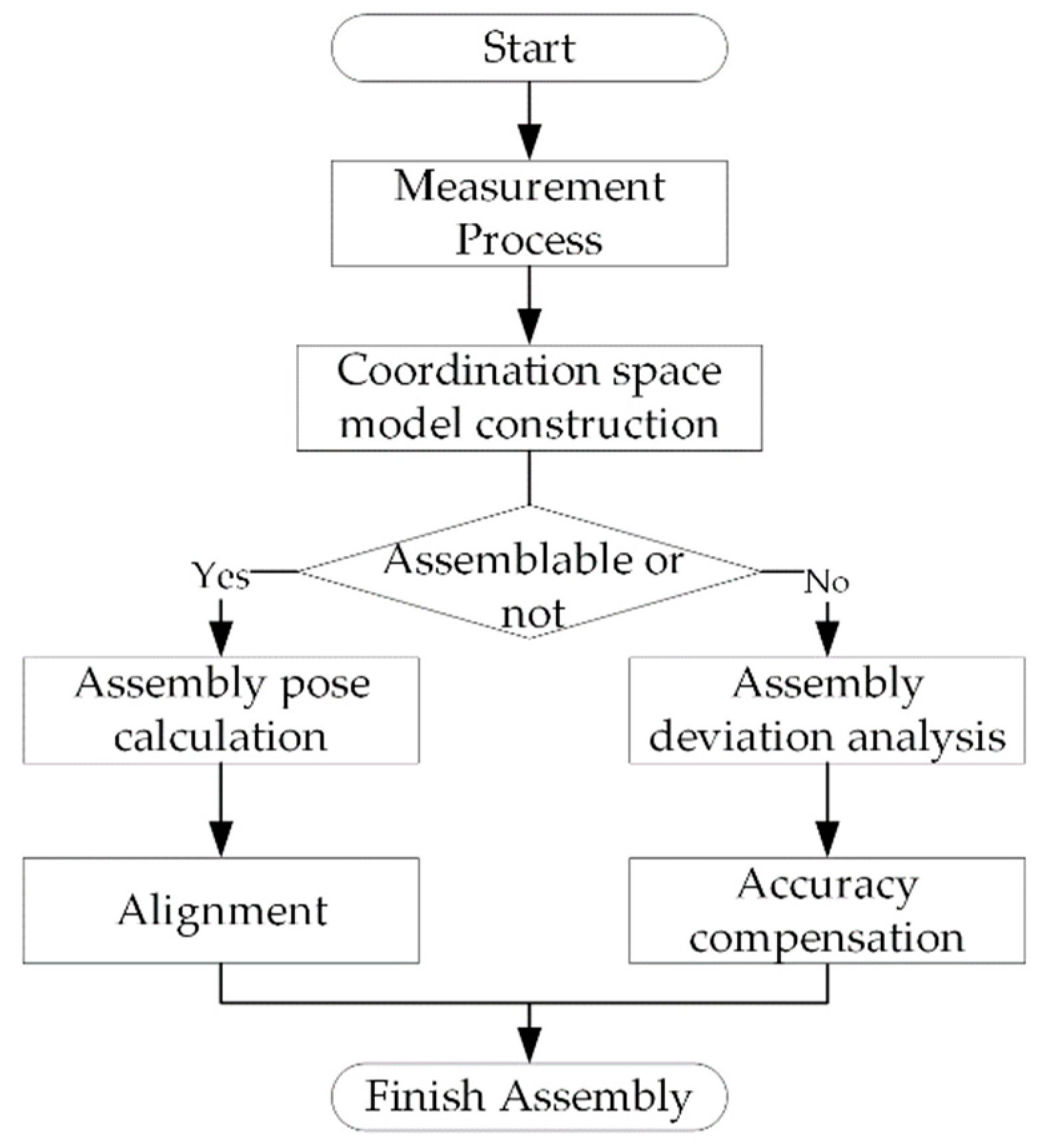
3. Assemblability Analysis Based on Coordination Space Model

Assemblability refers to the geometric consistency of the matching geometric structures of the two assembling parts. It can be judged whether the assembly can directly be carried out by assemblability prediction.

The assemblability is good if the coordination space is greater than 0, which means at least one pose conforms to Equation (15). Otherwise, the assemblability is bad. Therefore, the assemblability analysis flow is shown in Figure 5.

Firstly, the KACs are measured by a laser tracker or other digital measurement devices. Then, the coordination space model is constructed based on the assembly accuracy requirements. The volume of the coordination space is solved to judge whether it is assemblable. It will be assemblable when ${\varnothing }_{CS}$ is greater than 0. The assembly can be executed by calculating the optimal pose and aligning the parts. It will be uncoordinated when ${\varnothing }_{CS}$ is 0. Then, the assembly deviation should be analyzed and compensated to make it assemblable.

The solution process of the coordination space is based on the Monte Carlo method:

• Calculate the optimal pose based on the least-squares method.
• According to the dimensions and assembly accuracy requirements, a maximum pose space is assumed, as Equation (16) shows. All poses out of the space are not valid for any assembly accuracy requirements.

  $${\mathit{\omega }}_{\mathrm{d}}:\left(-x_{\mathrm{d}},-y_{\mathrm{d}},-z_{\mathrm{d}},-{\alpha }_{\mathrm{d}},-{\beta }_{\mathrm{d}},-{\gamma }_{\mathrm{d}}\right)\to \left(x_{\mathrm{d}},y_{\mathrm{d}},z_{\mathrm{d}},{\alpha }_{\mathrm{d}},{\beta }_{\mathrm{d}},{\gamma }_{\mathrm{d}}\right),$$

  (16)
• Generate a random SDT uniformly for ${\mathrm{n}}_T$ times and check the SDTs by Equation (15).
• If ${\mathrm{n}}_j$ of ${\mathrm{n}}_T$ SDTs are valid, the coordination space is

  $${\varnothing }_{CS}=\frac{{\mathrm{n}}_j}{{\mathrm{n}}_T}64x_{\mathrm{d}}{y}_{\mathrm{d}}{z}_{\mathrm{d}}{\alpha }_{\mathrm{d}}{\beta }_{\mathrm{d}}{\gamma }_{\mathrm{d}},$$

  (17)

In the case of incoordination, the coordination space should be further analyzed. According to Equation (15), the coordination space is the intersection of KAC’s constraint equations. All constraints are divided by KACs. Equation (15) will be translated to

$$\left\{{\omega }_{\mathsf{\Delta }}|\begin{array}{c}\forall f_j^1\left({\mathit{K}}_1^R,{\mathit{K}}_1^A{\mathit{\omega }}_{\mathsf{\Delta }}^H\right)\in \left[T_j^{1-min},T_j^{1-max}\right],j\in \left[1,j_1\right],\\ \forall f_j^2\left({\mathit{K}}_2^R,{\mathit{K}}_2^A{\mathit{\omega }}_{\mathsf{\Delta }}^H\right)\in \left[T_j^{2-min},T_j^{2-max}\right],j\in \left[1,j_2\right],\\ \dots \\ \forall f_j^n\left({\mathit{K}}_n^R,{\mathit{K}}_n^A{\mathit{\omega }}_{\mathsf{\Delta }}^H\right)\in \left[T_j^{n-min},T_j^{n-max}\right],j\in \left[1,j_n\right]\end{array}\right\},$$

(18)

Let

$${\varnothing }_i^{KAC}=\left\{{\omega }_{\mathsf{\Delta }}^{i-KAC}|\begin{array}{c}\forall f_j^i\left({\mathit{K}}_i^R,{\mathit{K}}_i^A{\mathit{\omega }}_{\mathsf{\Delta }}^H\right)\in \left[T_j^{i-min},T_j^{i-max}\right],j\in \left[1,j_i\right]\end{array}\right\},$$

(19)

where ${\varnothing }_i^{KAC}$ is the KAC coordination space formed by the assembly accuracy requirements of a KAC, and ${\mathit{\omega }}_{\mathsf{\Delta }}^{i-KAC}$ is an SDT in the KAC coordination space. The ${\varnothing }_{CS}$ would be

$${\varnothing }_{CS}={\bigcap }_{i=1}^n{\varnothing }_i^{KAC},$$

(20)

The relationship between the KAC coordination space and the assembly coordination space is shown in Figure 6a.

Figure 6b shows the status of the KAC coordination space when the assembly is uncoordinated. Each area of the same color represents a KAC coordination space. The divided zone is named the coordination zone. The accuracy compensation method is needed to improve the assemblability.

According to Figure 6b, set the union of KAC coordination space as a union coordination space. It is formulated as

$${\varnothing }_{UCS}={\bigcup }_{i=1}^n{\varnothing }_i^{KAC},$$

(21)

where ${\varnothing }_{UCS}$ is the union coordination space. In the union coordination space, all poses are valid for some KACs but not valid for all. Some divided zones are valid for more KACs than others, e.g., the two zones marked with 3 are better than those marked with 1 or 2. The marked number is named the coordination zone index, which is the valid KACs′ number in the coordination zone. If a pose in the zone marked with 3 is selected, only one KAC needs to be compensated. In this way, an assemblability optimization method is put forward by selecting a coordination zone with larger volume and KAC number. The larger volume means a better geometric consistency, and the larger KAC number means fewer KACs need to be compensated.

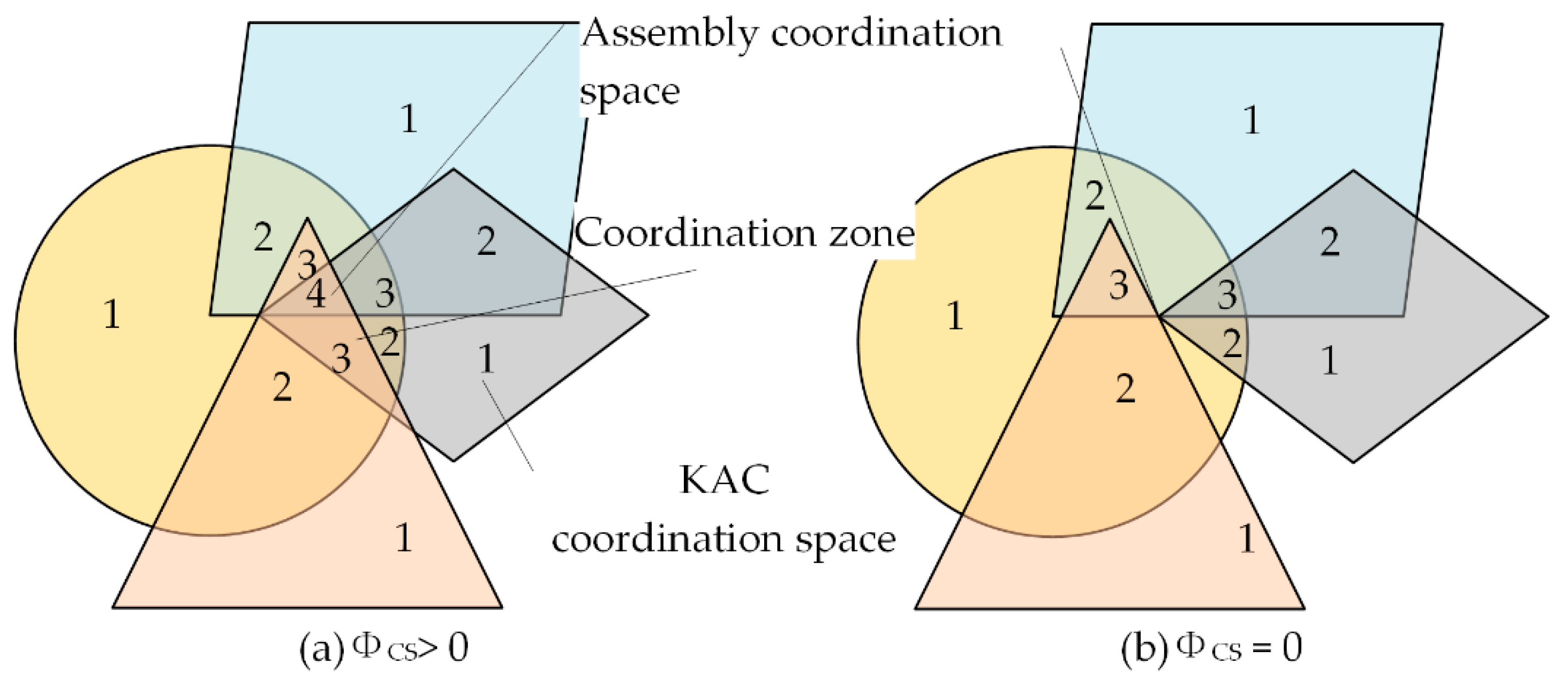
4. Assemblability Optimization Based on the Union Coordination Space

The accuracy compensation process is time- and effort- consuming [22] when the assemblability is poor. For example, it needs programming, clamping, tool setting, machining, loosen clamping, and other steps when finishing a KAC with cutting. Therefore, reducing the number of KACs to be processed is an effective means to improve the assembly efficiency in many cases. The optimal pose is usually obtained under the condition of optimal assembly accuracy. If each unqualified KAC is compensated one by one under the optimal pose, more work may be needed and the assembly quality might not be good, due to the unknown assembly quality after accuracy compensation. If the assembly quality is bad after compensation, there are no alternative compensation schemes based on the least-squares method. Therefore, the assemblability optimization method is proposed to solve the incoordination problem. The key to optimize the assemblability is whether there is one or more coordination zones that can satisfy assembly accuracy requirements with fewer KACs to be compensated and a better or approximate volume of coordination space.

The coordination zone index shows the valid KACs in the certain coordination zone. The total number of all KACs is $n_{KAC}$. The incoordination zone index shows the number of uncoordinated KACs in the coordination zone. Their relationship is

$$n_{IZI}=n_{KAC}-n_{CZI},$$

(22)

where $n_{IZI}$ is the incoordination zone index and $n_{CZI}$ is the coordination zone index. If the accuracy of uncoordinated KACs is compensated well in the coordination zone, this coordination zone will change to the assembly coordination space, as Figure 7 shows.

In this way, each coordination zone can be analyzed to check whether it is good to be compensated or not. Two indicators of the coordination zone should be analyzed, one is the incoordination zone index, and the other is the volume of the coordination zone. The Monte Carlo method of Section 3 is improved to judge the state of each coordination zone one by one, and the optimal assemblability optimization schemes of the coordination zone are selected for recording.

The solution process based on the Monte Carlo method is as follows:

• Solve the optimal pose of the align part;
• Set a pose space as the pose boundary as shown by the square box of Figure 8;
• Generate a random SDT in the pose space;
• According to Equation (19), judge which KAC equations are satisfied (coordination zone index) and which are not (incoordination zone index);
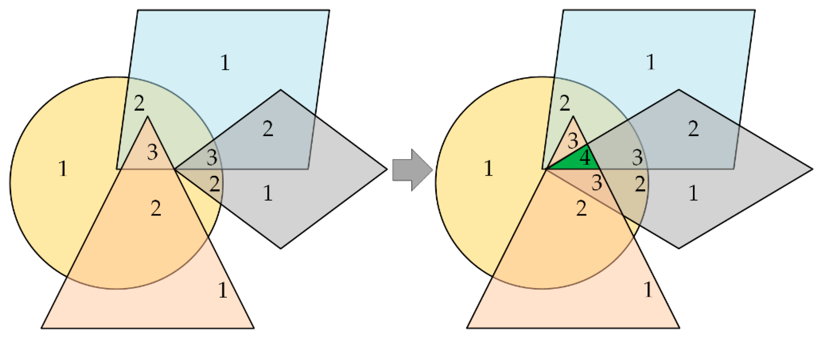
• Cluster the analysis results of each SDT. The SDTs in the same coordination zone are clustered together;
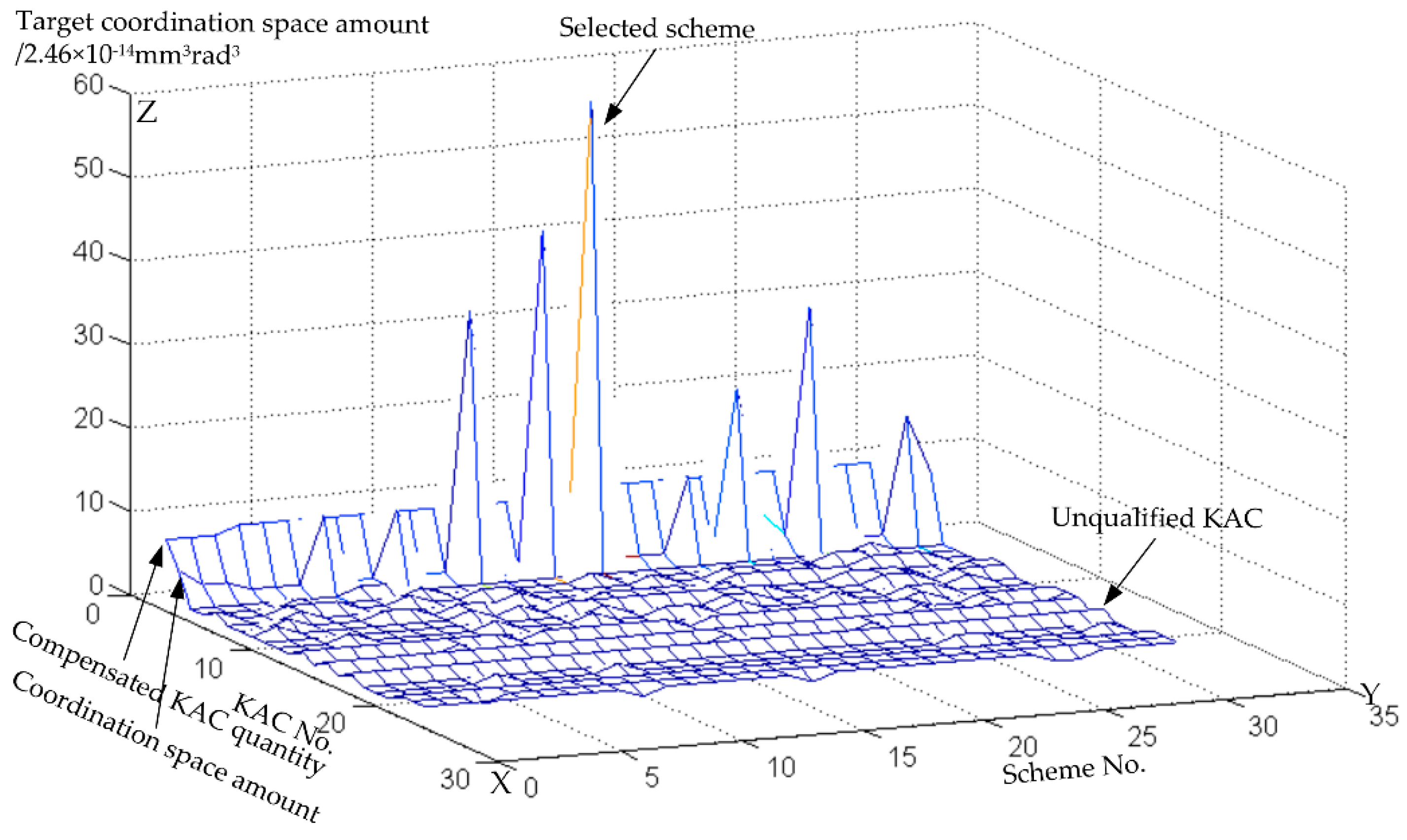
• Put the clustered results into the data structure of Equation (23). The KAC number to be compensated is the incoordination zone index. Select the scheme with a better KAC number and space volume of the coordination zone.

  $$\left\{{\mathsf{\Gamma }|\mathsf{\Gamma }}_i=\left(n_{IZI},V_{CZ},b_f,s_{\omega }\right),i<{\mathsf{\Gamma }}_{num}\right\},$$

  (23)

  where ${\mathsf{\Gamma }}_i$ is the ith scheme, $n_{IZI}$ is the incoordination zone index, $V_{\mathrm{CZ}}$ is the space amount of the coordination zone, $b_f$ is the information of uncoordinated KACs, $s_{\omega }$ is the SDT set, and ${\mathsf{\Gamma }}_{num}$ is the max number of the schemes.
• Calculate the center SDT of the SDTs in the selected scheme. The assembly deviation of target features under the SDT is analyzed and the accuracy compensation is carried out.

  $${\mathit{\omega }}_{\mathsf{\Delta }}^c=\frac{1}{n_s}{\sum }_{i=1}^{n_s}{\mathit{\omega }}_{\mathsf{\Delta }\mathrm{i}},$$

  (24)

  where ${\mathit{\omega }}_{\mathsf{\Delta }}^c$ is the center SDT, $n_s$ is the SDT number of $s_{\omega }$, and ${\mathit{\omega }}_{\mathsf{\Delta }\mathrm{i}}$ is an SDT of $s_{\omega }$. All assembly accuracies on ${\mathit{\omega }}_{\mathsf{\Delta }}^c$ are calculated. Then, the deviations on the excessive KACs will be compensated.

According to Equations (13) and (24), the compensation amount would be

$$C_j^i=T_j^{i-{\mathsf{\omega }}_{\mathsf{\Delta }}^c}-T_j^{i-\mathrm{opt}}=f_j^i\left({\mathit{K}}_i^R,{\mathit{K}}_i^A{\mathit{\omega }}_{\mathsf{\Delta }}^c\right)-T_j^{i-\mathrm{opt}},$$

(25)

where $C_j^i$ is the compensation amount of the jth assembly accuracy requirement of the ith KAC, $T_j^{i-{\omega }_{\mathsf{\Delta }}^c}$ is the assembly accuracy on the SDT ${\omega }_{\mathsf{\Delta }}^c$, and $T_j^{i-\mathrm{opt}}$ is the optimal value of the assembly accuracy.

5. Case Study

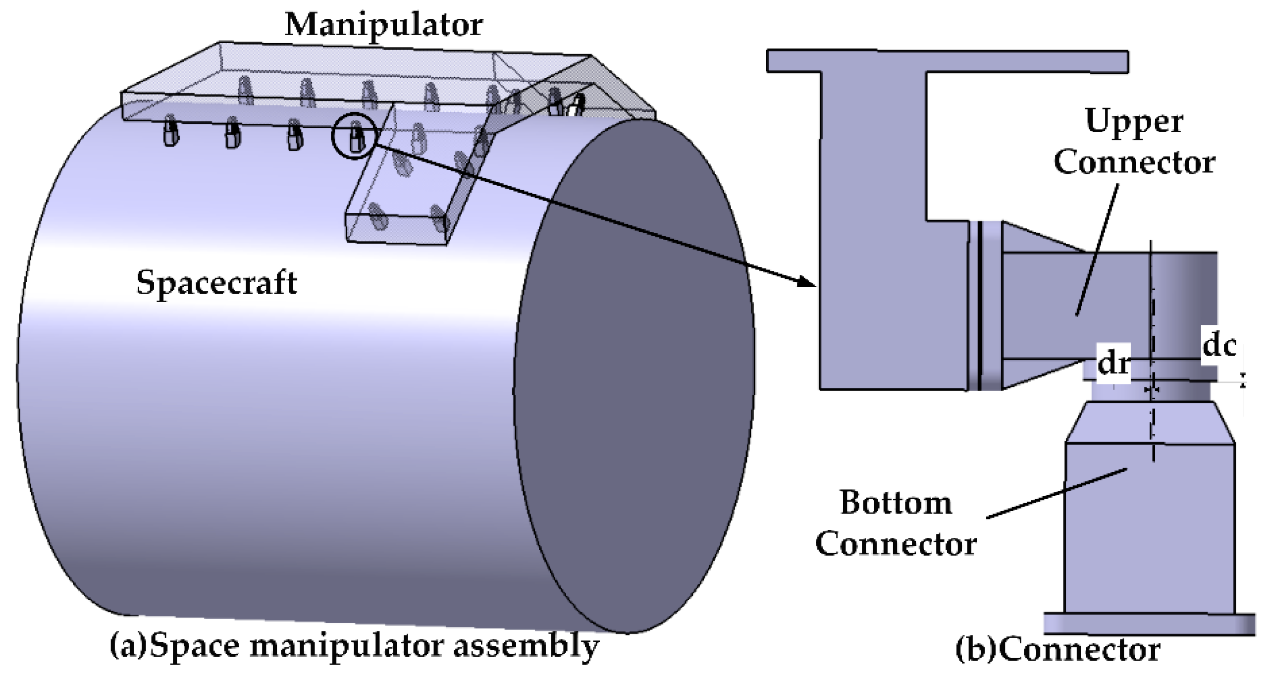
5.1. Space Manipulator Assembly

The space manipulator is fixed on the spacecraft, which needs a high assembly accuracy to guarantee the stability when the spacecraft is flying. The assembly is executed by shaft and hole connectors, which are shown in Figure 9a. The connector is shown in Figure 9b. The manipulator is the align part and the spacecraft is the reference part.

The upper connector is fixed on the manipulator, and the bottom connector is fixed on the spacecraft. The KACs are the assembly of the connectors. Due to the slight deformation of the spacecraft and the installation error of the bottom connectors, it is difficult for the connectors to accurately assemble at one time during the assembly of the spacecraft and the manipulator. In the original assembly process, it is necessary to try the assembly first, measure the assembly deviation of the clearance and coaxiality of each pair of connectors, make the accuracy compensation, and retry the assembly to ensure the assembly quality. The assembly takes a long time and the connectors are not convenient to be operated on the spacecraft. Therefore, the laser tracker is used to measure the connectors between the spacecraft and the manipulator. The methods in Section 2 and Section 3 are taken to evaluate the assemblability based on the measurement data. The method in Section 4 is used to find the key connectors to make the accuracy compensation. The assembly is carried out after the accuracy compensation. In this way, the assembly quality is better guaranteed and the assembly efficiency is improved. The flow of the proposed method and the comparison with the original method are shown in Figure 10.

As shown in Figure 10, the assembly process is developed toward digital measurement and analysis. The results obtained in the actual assembly and inspection are replaced by the analysis of the measurement data. Therefore, some unnecessary assembly processes are eliminated and the possibility of repeated trial assembly is greatly reduced.

The assembly accuracy requirements of the connector are coaxiality $dr$ and clearance $dc$ on the matching surface, as shown in Figure 9b. The coaxiality requirement is 0.2 mm, and the clearance requirement is 0.1 mm. Assembly accuracy is compensated by gasket compensation, finishing, or position movement according to the deviation.

5.2. Coordination Space Model

The measurement of the connector is based on the measurement auxiliary tool, which is shown in Figure 11.

After inserting the shaft into the corresponding hole, measure the four holes of the measurement auxiliary tool. The measurement data are processed as the position $p$ and orientation $\stackrel{\rightharpoonup }{po}$.

$$\{\begin{array}{c}\stackrel{\rightharpoonup }{\mathit{p}\mathit{o}}=\frac{\left({\mathit{c}}_3-{\mathit{c}}_1\right)\times \left({\mathit{c}}_4-{\mathit{c}}_2\right)}{\left|\left({\mathit{c}}_3-{\mathit{c}}_1\right)\times \left({\mathit{c}}_4-{\mathit{c}}_2\right)\right|}\\ \mathit{p}=\frac{1}{4}\sum {\mathit{c}}_i-l·\stackrel{\rightharpoonup }{\mathit{p}\mathit{o}}\end{array},$$

(26)

where ${\mathit{c}}_1$, ${\mathit{c}}_2$, ${\mathit{c}}_3$, and ${\mathit{c}}_4$ are the points measured by the laser tracker.

As shown in Figure 12, the clearance $dc$ and the coaxiality $dr$ of a connector are

$$\{\begin{array}{c}dr=\left|\stackrel{\rightharpoonup }{{\mathit{p}}_2{\mathit{p}}_1}·sin{\theta }_2\right|\\ dc=\left|\stackrel{\rightharpoonup }{{\mathit{p}}_1{\mathit{p}}_2}\right|·cos{\theta }_2+r·sin\left({\theta }_2-{\theta }_1\right)\end{array},$$

(27)

where ${\theta }_1$ and ${\theta }_2$ are the angles between $\stackrel{\rightharpoonup }{{\mathit{p}}_1{\mathit{p}}_2}$ and $\stackrel{\rightharpoonup }{{\mathit{p}}_1{\mathit{o}}_1}$ or $\stackrel{\rightharpoonup }{{\mathit{p}}_1{\mathit{o}}_2}$; ${\theta }_1$ can be calculated by ${\theta }_1=arccos\left(\stackrel{\rightharpoonup }{{\mathit{p}}_1{\mathit{p}}_2}·\stackrel{\rightharpoonup }{{\mathit{p}}_1{\mathit{o}}_1}/\left|\stackrel{\rightharpoonup }{{\mathit{p}}_1{\mathit{p}}_2}\right|\left|\stackrel{\rightharpoonup }{{\mathit{p}}_1{\mathit{o}}_1}\right|\right)$ and, similarly, ${\theta }_2$ can be calculated by the same way; and $r$ is the radius of the matching surface, which is 15 mm. There are 20 connectors to be guaranteed at the same time.

Therefore, the coordination space model is

$$\left\{{\mathit{\omega }}_{\mathsf{\Delta }}|\begin{array}{c}\left|\stackrel{\rightharpoonup }{{\mathit{p}}_2^{i-{\omega }_{\mathsf{\Delta }}}{\mathit{p}}_1^i}{\mathit{\omega }}_{\mathsf{\Delta }}^H·sin{\theta }_2^{i-{\omega }_{\mathsf{\Delta }}}\right|<0.2,\\ 0<\left|\stackrel{\rightharpoonup }{{\mathit{p}}_1^i{\mathit{p}}_2^{i-{\omega }_{\mathsf{\Delta }}}}\right|·cos{\theta }_2^{i-{\omega }_{\mathsf{\Delta }}}+r·sin\left({\theta }_2^{i-{\omega }_{\mathsf{\Delta }}}-{\theta }_1^{i-{\omega }_{\mathsf{\Delta }}}\right)<0.1,\\ i\in \left[1,20\right]\end{array}\right\},$$

(28)

where ${\mathit{\omega }}_{\mathsf{\Delta }}$ is the random SDT based on the optimal pose derived from the least-squares method, and ${\mathit{p}}_2^{i-{\omega }_{\mathsf{\Delta }}}$ is the parameters of Equation (27) changed by ${\mathit{\omega }}_{\mathsf{\Delta }}$ according to Equation (12), which are listed in Equation (29):

$$\{\begin{array}{c}{\mathit{p}}_2^{i-{\omega }_{\mathsf{\Delta }}}={\mathit{p}}_2^i{\mathit{\omega }}_{\mathsf{\Delta }}^H\\ \stackrel{\rightharpoonup }{{\mathit{p}}_2^{i-{\omega }_{\mathsf{\Delta }}}{\mathit{o}}_2^{i-{\omega }_{\mathsf{\Delta }}}}=\frac{\left({\mathit{c}}_3^i-{\mathit{c}}_1^i\right)\times \left({\mathit{c}}_4^i-{\mathit{c}}_2^i\right)}{\left|\left({\mathit{c}}_3^i-{\mathit{c}}_1^i\right)\times \left({\mathit{c}}_4^i-{\mathit{c}}_2^i\right)\right|}\\ {\theta }_1^{i-{\omega }_{\mathsf{\Delta }}}=arccos\left(\stackrel{\rightharpoonup }{{\mathit{p}}_1^l{\mathit{p}}_2^{l-{\omega }_{\mathsf{\Delta }}}}·\stackrel{\rightharpoonup }{{\mathit{p}}_1^l{\mathit{o}}_1^l}/\left|\stackrel{\rightharpoonup }{{\mathit{p}}_1^l{\mathit{p}}_2^{l-{\omega }_{\mathsf{\Delta }}}}\right|\left|\stackrel{\rightharpoonup }{{\mathit{p}}_1^l{\mathit{o}}_1^l}\right|\right)\\ {\theta }_2^{i-{\omega }_{\mathsf{\Delta }}}=arccos\left(\stackrel{\rightharpoonup }{{\mathit{p}}_1^l{\mathit{p}}_2^{l-{\omega }_{\mathsf{\Delta }}}}·\stackrel{\rightharpoonup }{{\mathit{p}}_2^{l-{\omega }_{\mathsf{\Delta }}}{\mathit{o}}_2^{l-{\omega }_{\mathsf{\Delta }}}}/\left|\stackrel{\rightharpoonup }{{\mathit{p}}_1^l{\mathit{p}}_2^{l-{\omega }_{\mathsf{\Delta }}}}\right|\left|\stackrel{\rightharpoonup }{{\mathit{p}}_2^{l-{\omega }_{\mathsf{\Delta }}}{\mathit{o}}_2^{l-{\omega }_{\mathsf{\Delta }}}}\right|\right)\end{array},$$

(29)

5.3. Assemblability Analysis

Part of the raw data is listed in

Table 1. Part of the raw measurement data.

Spacecraft			Manipulator
x/mm	y/mm	z/mm	x/mm	y/mm	z/mm
26.060	26.037	−192.674	222.509	2274.256	403.730
25.941	−25.881	−192.645	222.471	2222.338	403.647
−25.972	−25.945	−192.558	170.389	2222.349	403.666
−25.973	26.032	−192.581	170.520	2274.362	403.722

. All the measurement data are listed in Appendix A,

Table A1. Raw measurement data.

Spacecraft			Spacecraft			Manipulator			Manipulator
x/mm	y/mm	z/mm	x/mm	y/mm	z/mm	x/mm	y/mm	z/mm	x/mm	y/mm	z/mm
26.060	26.037	−192.674	2525.979	25.966	−192.595	222.509	2274.256	403.730	2722.472	2274.418	403.607
25.941	−25.881	−192.645	2525.879	−26.066	−192.588	222.471	2222.338	403.647	2722.406	2222.370	403.680
−25.972	−25.945	−192.558	2473.905	−25.939	−192.634	170.389	2222.349	403.666	2670.395	2222.418	403.611
−25.973	26.032	−192.581	2473.927	26.032	−192.648	170.520	2274.362	403.722	2670.399	2274.318	403.725
25.964	−1103.891	−192.620	2525.886	−1103.863	−192.642	222.163	1144.197	403.734	2722.221	1144.019	403.649
25.995	−1155.853	−192.533	2525.963	−1155.983	−192.687	222.172	1092.171	403.594	2722.191	1092.064	403.681
−26.108	−1155.891	−192.633	2473.910	−1155.938	−192.617	170.261	1092.242	403.670	2670.236	1092.093	403.632
−26.138	−1103.914	−192.600	2473.997	−1103.946	−192.532	170.240	1144.209	403.636	2670.134	1144.022	403.682
526.046	26.182	−192.691	25.984	371.512	−292.868	722.540	2274.127	403.704	222.310	2619.620	303.466
526.032	−25.859	−192.578	26.082	328.937	−322.879	722.525	2222.138	403.647	222.406	2577.169	273.462
474.044	−25.874	−192.632	−25.948	328.968	−322.927	670.477	2222.107	403.660	170.271	2577.228	273.409
473.999	26.048	−192.660	−25.989	371.392	−292.860	670.519	2274.160	403.749	170.259	2619.691	303.502
525.926	−1103.994	−192.665	26.306	779.693	−581.183	722.553	1144.152	403.622	222.373	3028.126	15.112
525.941	−1156.028	−192.670	26.328	737.195	−611.193	722.582	1092.046	403.733	222.475	2985.706	−14.926
473.906	−1155.956	−192.534	−25.677	737.131	−611.127	670.483	1092.007	403.687	170.440	2985.796	−14.932
474.001	−1103.938	−192.549	−25.718	779.531	−581.201	670.468	1144.107	403.701	170.438	3028.159	15.042
1025.900	25.892	−192.696	526.057	371.467	−292.910	1222.170	2274.325	403.687	722.232	2619.736	303.446
1025.991	−26.042	−192.675	525.980	329.046	−322.917	1222.300	2222.253	403.652	722.264	2577.274	273.375
973.956	−26.131	−192.596	473.953	329.017	−322.836	1170.188	2222.222	403.641	670.255	2577.165	273.441
973.988	25.990	−192.571	473.989	371.499	−292.943	1170.178	2274.330	403.697	670.274	2619.662	303.464
1026.139	−1104.097	−192.694	526.004	779.757	−581.219	1222.329	1144.177	403.676	722.338	3027.977	14.999
1026.085	−1156.050	−192.740	525.882	737.293	−611.181	1222.380	1092.031	403.649	722.348	2985.465	−14.896
974.124	−1156.044	−192.605	474.011	737.365	−611.149	1170.291	1092.073	403.617	670.334	2985.461	−14.882
974.105	−1104.011	−192.634	474.022	779.818	−581.198	1170.331	1144.076	403.725	670.270	3028.053	15.054
1525.925	26.129	−192.717	25.959	−1458.921	−322.909	1722.341	2274.278	403.722	222.442	789.300	273.358
1525.908	−25.848	−192.628	26.022	−1501.395	−292.846	1722.343	2222.377	403.704	222.364	746.770	303.402
1473.914	−25.921	−192.601	−26.061	−1501.356	−292.887	1670.349	2222.277	403.637	170.403	746.817	303.352
1473.942	26.171	−192.663	−25.980	−1458.862	−322.971	1670.315	2274.352	403.667	170.462	789.233	273.423
1526.063	−1104.006	−192.639	26.112	−1867.403	−611.275	1722.264	1144.106	403.701	222.487	380.493	−14.929
1525.951	−1155.886	−192.590	25.999	−1909.862	−581.157	1722.267	1092.232	403.641	222.479	338.017	15.121
1473.970	−1155.991	−192.610	−25.945	−1909.883	−581.133	1670.247	1092.136	403.697	170.454	337.946	15.019
1474.029	−1103.917	−192.536	−25.952	−1867.415	−611.214	1670.338	1144.104	403.578	170.502	380.501	−15.022
2026.006	25.807	−192.610	525.901	−1459.048	−322.918	2222.301	2274.138	403.623	722.541	789.350	273.516
2026.008	−26.174	−192.602	525.980	−1501.511	−292.844	2222.194	2222.153	403.685	722.525	746.885	303.481
1974.072	−26.202	−192.597	474.025	−1501.571	−292.828	2170.273	2222.082	403.688	670.449	746.930	303.374
1973.940	25.758	−192.615	473.983	−1459.106	−322.849	2170.301	2274.070	403.707	670.465	789.270	273.409
2025.839	−1103.981	−192.592	525.886	−1867.434	−611.169	2222.555	1144.297	403.746	722.630	380.599	−14.830
2025.808	−1155.974	−192.526	525.806	−1909.943	−581.114	2222.521	1092.226	403.623	722.554	338.263	15.129
1973.868	−1155.897	−192.571	473.872	−1909.917	−581.157	2170.597	1092.349	403.654	670.639	338.232	15.073
1973.894	−1103.986	−192.651	473.840	−1867.343	−611.211	2170.608	1144.349	403.683	670.507	380.619	−14.907

.

The least-squares method is taken to calculate the optimal pose and the deviations on the optimal pose. The deviations of the connectors are listed in

Table 2. Assembly deviation prediction by least-squares method.

No.	dr/mm	dc/mm	No.	dr/mm	dc/mm
1	0.154	0.043	11	0.171	−0.012
2	0.150	−0.027	12	0.338	0.002
3	0.205	0.072	13	0.286	−0.010
4	0.196	0.042	14	0.530	−0.274
5	0.191	0.012	15	0.247	0.033
6	0.209	0.083	16	0.165	−0.029
7	0.066	0.045	17	0.188	0.033
8	0.195	−0.025	18	0.402	−0.154
9	0.118	−0.006	19	0.086	0.183
10	0.298	−0.010	20	0.386	−0.028

calculated by Equation (27).

It can be seen that 10 connectors need to be adjusted or repaired based on the least-squares method.

The coordination space is 0 at the optimal pose based on the method in Section 3, which means it cannot be assembled directly. Therefore, the assemblability should be optimized.

5.4. Assemblability Optimization

The proposed method in Section 4 is taken to find the accuracy compensation schemes. The results are shown in Figure 13.

Figure 13 shows the accuracy compensation schemes. The first point on the X axis is the KAC quantity to be compensated. The second point is the volume of the coordination zone of the scheme. The latter ones are the number of KACs. The Y axis is the scheme number. The Z axis is the value of the X axis. Seven connectors need to be adjusted to complete assembly in scheme 1. Finally, scheme 18, which needs nine connectors to be compensated, is taken by considering the assembly quality. The coordination space of the scheme is 56d. d is the volume of the maximum pose space divided by random times. In this case, d is $2.46\times {10}^{-14}{ \mathrm{mm}}^3{\mathrm{rad}}^3$. The KAC number to be compensated is 5, 6, 8, 10, 12, 14, 18, 19, and 20. The center SDT of the coordination zone in scheme 18 is $\left(-0.0363 \mathrm{mm},0.0210 \mathrm{mm},0.0098 \mathrm{mm},2.52\times {10}^{-6} \mathrm{rad},1.64\times {10}^{-6} \mathrm{rad},-2.35\times {10}^{-6} \mathrm{rad}\right)$.

The deviation is calculated under the center SDT listed in

Table 3. The deviations of the connectors.

No.	dr/mm	dc/mm	No.	dr/mm	dc/mm
1	0.145	0.034	11	0.150	−0.036
2	0.188	−0.031	12	0.351	−0.013
3	0.169	0.064	13	0.142	−0.022
4	0.151	0.031	14	0.391	−0.286
5	0.230	0.004	15	0.133	0.016
6	0.249	0.070	16	0.031	−0.039
7	0.025	0.037	17	0.056	0.032
8	0.222	−0.034	18	0.204	−0.145
9	0.162	−0.021	19	0.204	0.179
10	0.255	−0.029	20	0.233	−0.027

.

After simulation accuracy compensation for the above nine connectors, which is in bold and italics in Table 3 (the proposed method), the coordination space is 101d, which is greater than 0. The average coaxiality is 0.068 mm and the average clearance is 0.014 mm. The assemblability is good and the assembly can be executed directly.

After simulation accuracy compensation for the above 10 connectors, which is in bold and italics in Table 2 (the least square method), the coordination space is 9d. The average coaxiality is 0.084 mm and the average clearance is 0.014 mm. The assemblability is good but the assembly quality on coaxiality is worse.

The result shows that the proposed method will generate a better accuracy compensation scheme with less workload and better assembly quality, which improves the assemblability.

The measurement and connector adjustment process took about 8 h during the assembly. The pose adjustment process took about 2 h. Therefore, it took about 10 h in total based on the proposed method. The original assembly process took more than 20 h because the first trial assembly and accuracy compensation process cannot realize the re-trial assembly smoothly. Three or four times the assembly are needed to guarantee the assembly quality.

6. Discussion

Compared to the previous research, the major contributions in this paper are listed as follows: (1) The concept of assemblability and coordination accuracy in the design/drawing stage are extended into the measurement-assisted assembly. (2) An assemblability analysis method based on the measurement data and the coordination space model is proposed for predicting the key assembly deviations. (3) The accuracy compensation methods based on the optimal pose might lead to more workload and worse assemblability. Therefore, an assemblability optimization method is proposed for less workload and better assembly quality. In addition, the space manipulator assembly is taken as an example. The result shows that the proposed method can optimize the assemblability with less workload and better assembly quality compared to the accuracy compensation method based on the optimal pose.

The assemblability optimization method based on accuracy compensation improves the ability to detect assembly problems in advance, which will benefit the automation assembly. Further, the coordination space model and the small displacement torsor are useful for analyzing the assemblability and optimizing the tolerances in the design/drawings phase, but the assemblability optimization method is not useful. In the implementation of the method, high-precision digital measurement equipment are needed. Measurement uncertainty will affect the reliability of the final results.

Future research include evaluating the influence of the measurement uncertainty on the coordination space model. Then, the uncertainty of pose adjustment should be taken into consideration compared to the volume of the coordination space to judge the feasibility of automatic pose adjustment.

References

1. Zhou, F.; Xue, H.; Zhou, W.; Xu, G. Key technology and its improvement of aircraft digital flexible assembly. Aeronaut. Manuf. Technol. 2006, 9, 30–35. (In Chinese) [Google Scholar]
2. Maropoulos, P.G.; Muelaner, J.E.; Summers, M.D.; Martin, O.C. A new paradigm in large-scale assembly—Research priorities in measurement assisted assembly. Int. J. Adv. Manuf. Technol. 2014, 70, 621–633. [Google Scholar] [CrossRef] [Green Version]
3. Marguet, B.; Ribere, B. Measurement-assisted assembly applications on airbus final assembly lines. SAE Tech. Pap. 2003, 1, 2950. [Google Scholar]
4. Chen, Z.; Du, F.; Tang, X. Position and orientation best-fitting based on deterministic theory during large scale assembly. J. Intell. Manuf. 2015, 29, 827–837. [Google Scholar] [CrossRef]
5. Li, S.; Deng, Z.; Zeng, Q.; Huang, X. A coaxial alignment method for large aircraft component assembly using distributed monocular vision. Assem. Autom. 2018, 38, 437–449. [Google Scholar] [CrossRef]
6. Wang, Q.; Dou, Y.; Li, J.; Ke, Y.; Keogh, P.; Maropoulos, P.G. An assembly gap control method based on posture alignment of wing panels in aircraft assembly. Assem. Autom. 2017, 37, 422–433. [Google Scholar] [CrossRef] [Green Version]
7. Sukhan, L.; Chunsik, Y. Assemblability evaluation based on tolerance propagation. In Proceedings of the 1995 IEEE International Conference on Robotics and Automation, Nagoya, Japan, 21–27 May 1995. [Google Scholar]
8. Sanderson, A.C. Assemblability based on maximum likelihood configuration of tolerances. IEEE Trans. Robot. Autom. 1999, 15, 568–572. [Google Scholar] [CrossRef] [Green Version]
9. Cui, Z.; Du, F. Assessment of large-scale assembly coordination based on pose feasible space. Int. J. Adv. Manuf. Technol. 2019, 104, 4465–4474. [Google Scholar] [CrossRef]
10. Yuan, L.; Zhang, L.; Wang, Y. An optimal method of posture adjustment in aircraft fuselage joining assembly with engineering constraints. Chin. J. Aeronaut. 2017, 30, 222–229. [Google Scholar]
11. Wu, D.; Du, F. A Multi-constraints Based Pose Coordination Model for Large Volume Components Assembly. Chin. J. Aeronaut. 2019. [Google Scholar] [CrossRef]
12. Ma, H.; Jin, Y.; Zhang, X.; Zhou, H. Complex shape product tolerance and accuracy control method for virtual assembly. Proc. SPIE Int. Soc. Opt. Eng. 2015, 9446, 94462E. [Google Scholar]
13. Du, Q.; Zhai, X.; Wen, Q. Study of the Ultimate Error of the Axis Tolerance Feature and Its Pose Decoupling Based on an Area Coordinate System. Appl. Sci. 2018, 8, 435. [Google Scholar] [CrossRef] [Green Version]
14. Davis, B.; Jones, T.M.; Darrell, D.Z.; Tracy, E. Digitally Designed Shims for Joining Parts of an Assembly. European Patents EP 2533167A2, 5 June 2012. [Google Scholar]
15. Fabian, S.; Nathapon, O.L.; Jorg, W. Automated assembly of large CFRP structures: Adaptive filling of joining gaps with additive manufacturing. In Proceedings of the 2016 IEEE International Symposium on Assembly and Manufacturing, Fort Worth, TX, USA, 21–22 August 2016; pp. 126–132. [Google Scholar]
16. Wang, Q.; Dou, Y.; Cheng, L.; Ke, Y.; Qiao, H.; Zhao, X. Shimming design and optimal selection for non-uniform gaps in wing assembly. Assem. Autom. 2017, 37, 471–482. [Google Scholar] [CrossRef]
17. Muelaner, J.; Kayani, A.; Martin, O.; Maropoulos, P.G. Measurement assisted assembly and the roadmap to part-to-part assembly. In Proceedings of the DET2011 7th International Conference on Digital Enterprise Technology, Athens, Greece, 27–30 September 2011; pp. 11–19. [Google Scholar]
18. Cui, Z.; Du, F.; Xiong, T. Analysis and coordination on assembly deviation of multi plane-and-holes assembly based on orientation points groups. Acta Aeronaut. Astronaut. Sin. 2018, 38, 248–257. (In Chinese) [Google Scholar]
19. Yang, J.L.; Huang, X.; Li, L.; Xiong, T.; Zhao, Z. Method for extracting repair amount of skin seam based on scan line point cloud. Aeronaut. Manuf. Technol. 2019, 62, 73–77. (In Chinese) [Google Scholar]
20. Yu, A.; Liu, Z.; Duan, G.; Tan, J.; Che, L.; Chen, X. Geometric design model and object scanning mode based virtual assembly and repair analysis. Procedia CIRP 2016, 44, 144–150. [Google Scholar] [CrossRef] [Green Version]
21. Manohar, K.; Hogan, T.; Buttrick, J.; Banerjee, A.G.; Kutz, J.N.; Brunton, S.L. Predicting shim gaps in aircraft assembly with machine learning and sparse sensing. J. Manuf. Syst. 2018, 48, 87–95. [Google Scholar] [CrossRef]
22. Lei, P.; Zheng, L. An automated insitu alignment approach for finish machining assembly interfaces of large-scale components. Robot. Comput. Integr. Manuf. 2017, 46, 130–143. [Google Scholar] [CrossRef]
23. Cheng, B. Aircraft Manufacturing Coordination Accuracy and Tolerance Allocation, 1st ed.; Aviation Industry Press: Beijing, China, 1987; pp. 1–16. (In Chinese) [Google Scholar]
24. Arun, K.S. Least-squares fitting of two 3-D point sets. IEEE Trans. Pattern Anal. Mach. Intell. 1987, 9, 698–700. [Google Scholar] [CrossRef] [Green Version]
25. Liu, J.; Wang, T.; Zou, C. A blending control aircraft assembly quality method using key assembly characteristic. Adv. Mater. Res. 2011, 314–316, 2469–2473. [Google Scholar]
26. Bourdet, P.; Mathieu, L.; Lartigue, C.; Ballu, A. The concept of small displacement torsor in metrology. Adv. Math. Tools Metrol. 1996, 40, 110–122. [Google Scholar]
Figure 1. Coordination accuracy of a keyway assembly.
Applsci 10 03331 g001
Figure 2. The pose variations under the condition of assembly accuracy requirements.
Applsci 10 03331 g002
Figure 3. Wing-fuselage assembly.
Applsci 10 03331 g003
Figure 4. Valid poses of wing-fuselage assembly.
Applsci 10 03331 g004
Figure 5. Assemblability analysis process.
Applsci 10 03331 g005
Figure 6. The relationship between the part and feature PFS.
Applsci 10 03331 g006
Figure 7. The coordination zone variation process by accuracy compensation.
Applsci 10 03331 g007
Figure 8. Random sampling by Monte Carlo method.
Applsci 10 03331 g008
Figure 9. Space manipulator assembly.
Applsci 10 03331 g009
Figure 10. The comparison of the original and proposed assembly processes.
Applsci 10 03331 g010
Figure 11. Measurement auxiliary tool.
Applsci 10 03331 g011
Figure 12. Assembly geometric constraints analysis.
Applsci 10 03331 g012
Figure 13. The accuracy compensation schemes.
Applsci 10 03331 g013