Deep Inorganic Fraction Characterization of PM10, PM2.5, and PM1 in an Industrial Area Located in Central Italy by Means of Instrumental Neutron Activation Analysis


 , and
, and
Abstract
:1. Introduction
2. Materials and Methods
3. Results
3.1. Instrumental Neutron Activation Analysis (INAA) Validation
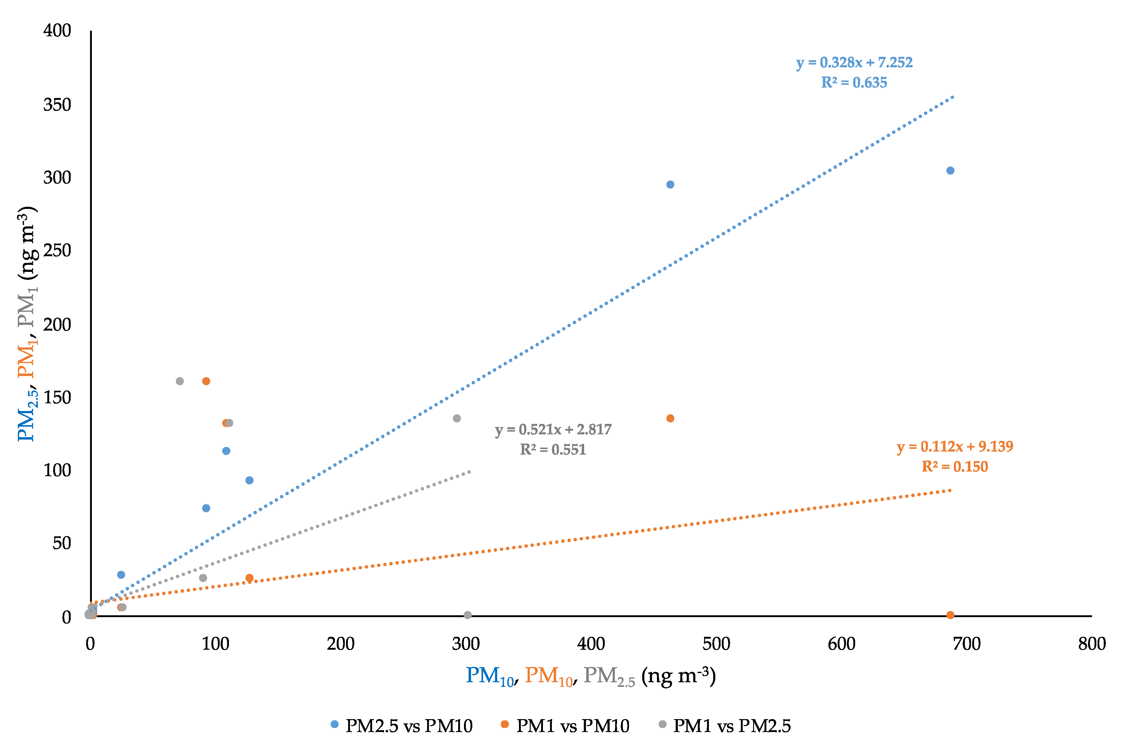
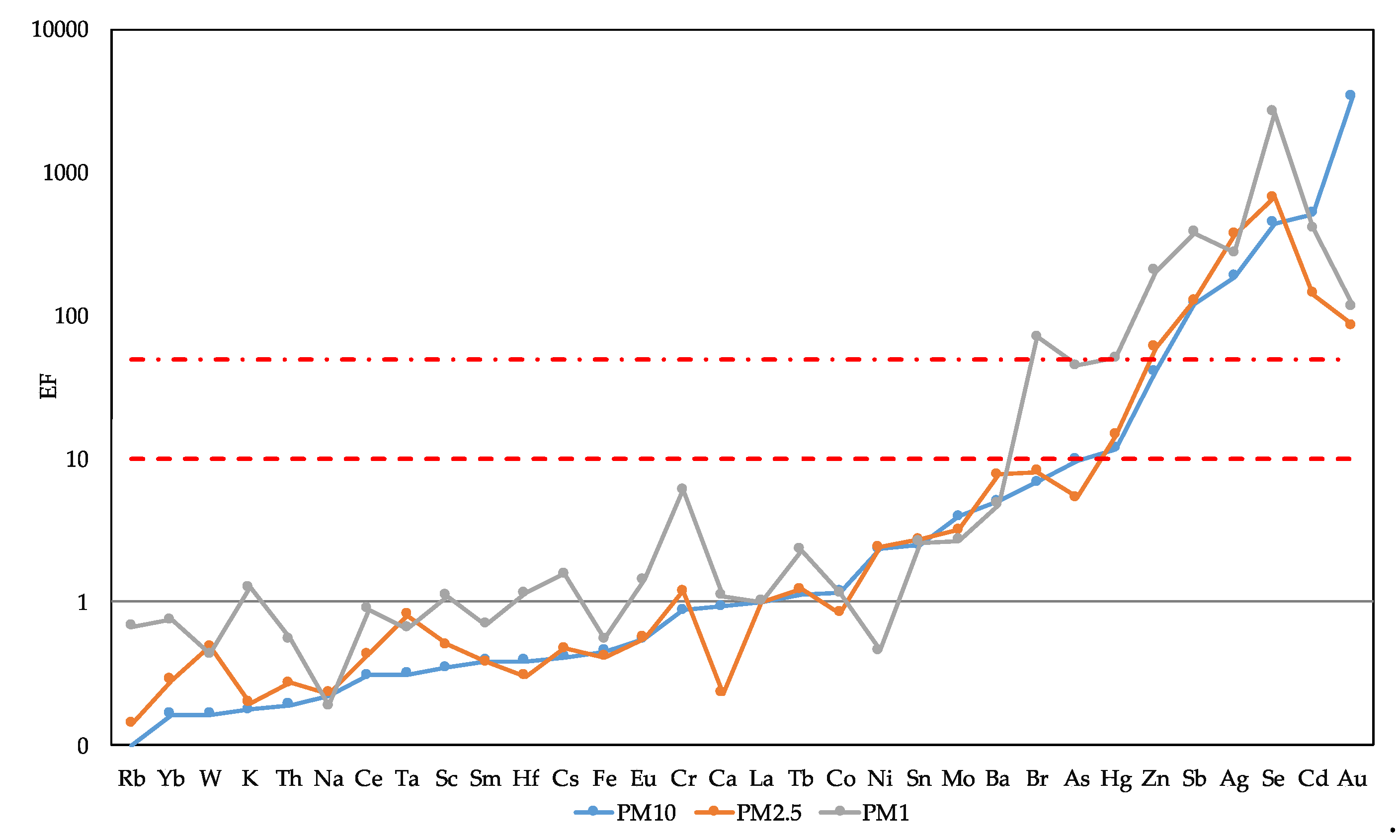
3.2. PM10, PM2.5, and PM1 Analysis
3.3. Comparison with Other Scenarios Worldwide
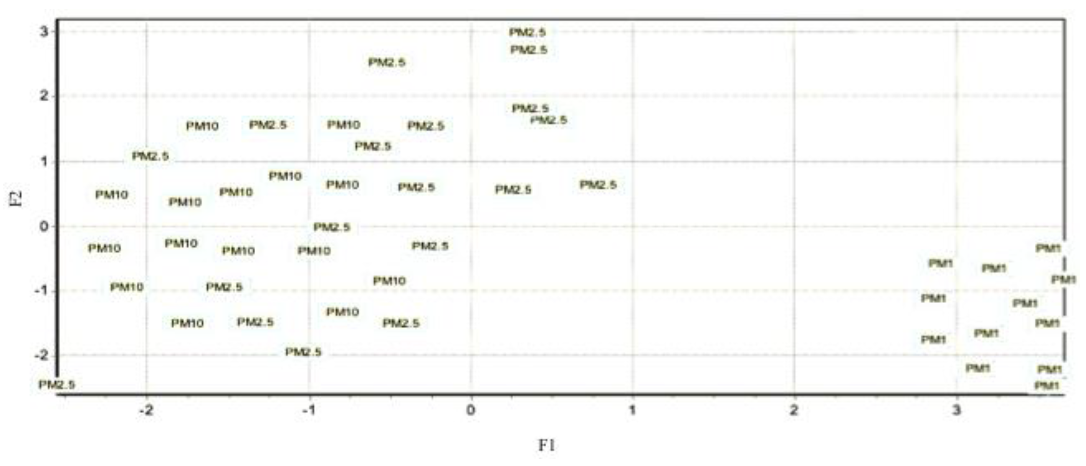
3.4. Statistical Analysis
- 1st Cluster (eleven members): W, Zn, Ba, Cr, Sc, Ag, Rb, Ce, Th, Sb, Ta.
- 2nd Cluster: (ten members): Br, Co, Eu, Sm, Mo, Se, Fe, Ni, Hf, Tb.
- 3rd Cluster (six members): As, Ca, Na, Cs, La, Au.
4. Conclusions
Author Contributions
Funding
Acknowledgments
Conflicts of Interest
References
- Avino, P.; Capannesi, G.; Rosada, A. Characterization and distribution of mineral content in fine and coarse airborne particle fractions by neutron activation analysis. Toxicol. Environ. Chem. 2006, 88, 633–647. [Google Scholar] [CrossRef]
- Avino, P.; Capannesi, G.; Rosada, A. Heavy metal determination in atmospheric particulate matter by Instrumental Neutron Activation Analysis. Microchem. J. 2008, 88, 97–106. [Google Scholar] [CrossRef]
- Alier, M.; Van Drooge, B.L.; Dall’Osto, M.; Querol, X.; Grimalt, J.; Tauler, R. Source apportionment of submicron organic aerosol at an urban background and a road site in Barcelona (Spain) during SAPUSS. Atmos. Chem. Phys. 2013, 20, 10353–10371. [Google Scholar] [CrossRef] [Green Version]
- Alolayan, M.A.; Brown, K.W.; Evans, J.S.; Bouhamra, W.S.; Koutrakis, P. Source apportionment of fine particles in Kuwait City. Sci. Total Environ. 2013, 448, 14–25. [Google Scholar] [CrossRef]
- Crippa, M.; Canonaco, F.; Slowik, J.G.; El Haddad, I.; Decarlo, P.F.; Mohr, C.; Heringa, M.F.; Chirico, R.; Marchand, N.; Temime-Roussel, B.; et al. Primary and secondary organic aerosol origin by combined gas-particle phase source apportionment. Atmos. Chem. Phys. 2013, 13, 8411–8426. [Google Scholar] [CrossRef] [Green Version]
- Mantas, E.; Remoundaki, E.; Halari, I.; Kassomenos, P.; Theodosi, C.; Hatzikioseyian, A.; Mihalopoulos, N. Mass closure and source apportionment of PM2.5 by Positive Matrix Factorization analysis in urban Mediterranean environment. Atmos. Environ. 2014, 94, 154–163. [Google Scholar] [CrossRef]
- Karagulian, F.; Belis, C.A.; Dora, C.F.C.; Prüss-Ustün, A.M.; Bonjour, S.; Adair-Rohani, H.; Amann, M. Contributions to cities’ ambient particulate matter (PM): A systematic review of local source contributions at global level. Atmos. Environ. 2015, 120, 475–483. [Google Scholar] [CrossRef]
- Manigrasso, M.; Febo, A.; Guglielmi, F.; Ciambottini, V.; Avino, P. Relevance of aerosol size spectrum analysis as support to qualitative source apportionment studies. Environ. Pollut. 2012, 170, 43–51. [Google Scholar] [CrossRef]
- Marini, S.; Buonanno, G.; Stabile, L.; Avino, P. A benchmark for numerical scheme validation of airborne particle exposure in street canyons. Environ. Sci. Pollut. Res. 2015, 22, 2051–2063. [Google Scholar] [CrossRef]
- Neuwahl, F.; Cusano, G.; Gómez Benavides, J.; Holbrook, S.; Roudier, S. Best Available Techniques (BAT) Reference Document for Waste Incineration; EUR 29971 EN; Publications Office of the European Union: Luxembourg, 2019; Available online: https://eippcb.jrc.ec.europa.eu/sites/default/files/2020-01/JRC118637_WI_Bref_2019_published_0.pdf (accessed on 10 February 2020). [CrossRef]
- Eurostat Statistical Books. Environmental Statistics and Accounts in Europe 2010; European Union: Strasbourg, France, 2010; Available online: https://ec.europa.eu/eurostat/documents/3217494/5723037/KS-32-10-283-EN.PDF/22a4889d-e6c9-4583-8d17-fb5104e7eec0 (accessed on 13 February 2020).
- European Commission. Review of the Thematic Strategy on the Prevention and Recycling of Waste; Commission Staff Working Document; European Commission: Brussels, Belgium, 2019; Available online: https://ec.europa.eu/environment/waste/strategy.htm (accessed on 20 January 2020).
- European Commission. Council Directive 2008/98/EC of 19 November 2008. Directive on waste and repealing certain Directives. Off. J. Eur. Union 2008, L312, 3–30. [Google Scholar]
- Cass, G.R.; Hughes, L.A.; Bhave, P.; Kleeman, M.J.; Allen, J.O.; Salmon, L.G. The chemical composition of atmospheric ultrafine particles. Philos. Trans. R. Soc. Lond. Ser. A 2000, 358, 2581–2592. [Google Scholar] [CrossRef]
- Ranzi, A.; Fustinoni, S.; Erspamer, L.; Campo, L.; Gatti, M.G.; Bechtold, P.; Bonassi, S.; Trenti, T.; Goldoni, C.A.; Bertazzi, P.A.; et al. Biomonitoring of the general population living near a modern solid waste incinerator: A pilot study in Modena, Italy. Environ. Int. 2013, 61, 88–97. [Google Scholar] [CrossRef] [PubMed]
- Allsopp, M.; Costner, P.; Johnston, P. Incineration and human health: State of knowledge of the impacts of waste incinerators on human health (executive summary). Environ. Sci. Pollut. Res. 2011, 8, 141–145. [Google Scholar] [CrossRef] [PubMed]
- Ranzi, A.; Fano, V.; Erspamer, L.; Lauriola, P.; Perucci, C.A.; Forastiere, F. Mortality and morbidity among people living close to incinerators: A cohort study based on dispersion modeling for exposure assessment. Environ. Health 2011, 10, 22. [Google Scholar] [CrossRef] [PubMed] [Green Version]
- Forastiere, F.; Badaloni, C.; De Hoogh, K.; von Kraus, M.K.; Martuzzi, M.; Mitis, F.; Palkovicova, L.; Porta, D.; Preiss, P.; Ranzi, A.; et al. Health impact assessment of waste management facilities in three European countries. Environ. Health 2011, 10, 53. [Google Scholar] [CrossRef] [Green Version]
- Cordioli, M.; Vincenzi, S.; De Leo, G.A. Effects of heat recovery for district heating on waste incineration health impact: A simulation study in Northern Italy. Sci. Total Environ. 2013, 444, 369–380. [Google Scholar] [CrossRef]
- Cordioli, M.; Ranzi, A.; De Leo, G.A.; Lauriola, P. A review of exposure assessment methods in epidemiological studies on incinerators. J. Environ. Public Health 2013, 2013, 129470. [Google Scholar] [CrossRef] [Green Version]
- Lee, C.C.; Huffman, G.L.; Oberacker, D.A. An overview of hazardous/toxic waste incineration. J. Air Pollut. Control Assoc. 1986, 36, 922–931. [Google Scholar] [CrossRef]
- Oppelt, E.T. Incineration of hazardous waste. JAPCA 1987, 37, 558–586. [Google Scholar] [CrossRef]
- USNRC. Waste Incineration and Public Health; Committee on Health Effects of Waste Incineration, Ed.; National Academy Press: Washington, DC, USA, 2000; Available online: https://www.nap.edu/catalog/5803/waste-incineration-and-public-health (accessed on 10 February 2020).
- Chen, Z.; Lin, X.; Lu, S.; Li, X.; Qiu, Q.; Wu, A.; Ding, J.; Yan, J. Formation pathways of PCDD/Fs during the co-combustion of municipal solid waste and coal. Chemosphere 2018, 20, 862–870. [Google Scholar] [CrossRef]
- Wang, G.; Deng, J.; Ma, Z.; Hao, J.; Jiang, J. Characteristics of filterable and condensable particulate matter emitted from two waste incineration power plants in China. Sci. Total Environ. 2018, 639, 695–704. [Google Scholar] [CrossRef] [PubMed]
- Buonanno, G.; Stabile, L.; Avino, P.; Vanoli, R. Dimensional and chemical characterization of particles at a downwind receptor site of a waste-to-energy plant. Waste Manag. 2010, 30, 1325–1333. [Google Scholar] [CrossRef] [PubMed]
- Buonanno, G.; Stabile, L.; Avino, P.; Belluso, E. Chemical, dimensional and morphological ultrafine particle characterization from a waste-to-energy plant. Waste Manag. 2011, 31, 2253–2262. [Google Scholar] [CrossRef] [PubMed]
- Nielsen, M.; Illerup, J.B. Emissionsfaktorer og Emissionsopgørelse for Decentral Kraftvarme, Eltra PSO Projekt 3141, Kortlægning Af Emissionsfaktorer Fra Decentral kraftvarme, Delrapport 6, 2003, nr. 442. Available online: http://www2.dmu.dk/1_viden/2_Publikationer/3_fagrapporter/rapporter/FR442.pdf (accessed on 20 January 2020).
- Nielsen, M.; Illerup, J.B.; Fogh, C.L.; Johansen, L.P. PM Emission from CHP Plants < 25MWe; National Environmental Research Institute of Denmark: Roskilde, Denmark, 2006; Available online: http://www2.dmu.dk/1_Viden/2_Miljoe-tilstand/3_luft/4_adaei/doc/Poster_Eltra_PM.doc (accessed on 20 January 2020).
- Capannesi, G.; Rosada, A.; Avino, P. Elemental characterization of impurities at trace and ultra-trace levels in metallurgical lead samples by INAA. Microchem. J. 2009, 93, 188–194. [Google Scholar] [CrossRef]
- Avino, P.; Capannesi, G.; Manigrasso, M.; Sabbioni, E.; Rosada, A. Element assessment in whole blood, serum and urine of three Italian healthy sub-populations by INAA. Microchem. J. 2011, 99, 548–555. [Google Scholar] [CrossRef]
- Avino, P.; Capannesi, G.; Renzi, L.; Rosada, A. Instrumental neutron activation analysis and statistical approach for determining baseline values of essential and toxic elements in hairs of high school students. Ecotoxicol. Environ. Saf. 2013, 92, 206–214. [Google Scholar] [CrossRef]
- EN 12341. Determination of the PM10 Fraction of Suspended Particulate Matter-Reference Method and Field Test Procedure to Demonstrate Reference Equivalence of Measurement Methods; European Commission: Strasbourg, France, 1988. [Google Scholar]
- Erdtmann, G.; Soyka, W. The Gamma Rays of the Radionuclides; Wiley-VCH: New York, NY, USA, 1988. [Google Scholar]
- Campanella, L.; Crescentini, G.; Avino, P.; Moauro, A. Determination of macrominerals and trace elements in the alga Spirulina platensis. Analusis 1998, 26, 210–214. [Google Scholar] [CrossRef]
- Avino, P.; Carconi, P.; Lepore, L.; Moauro, A. Nutritional and environmental properties of algal products used in healthy diet by INAA and ICP-AES. J. Radioanal. Nucl. Chem. 2000, 244, 247–252. [Google Scholar] [CrossRef]
- Seccaroni, C.; Volante, N.; Rosada, A.; Ambrosone, L.; Bufalo, G.; Avino, P. Identification of provenance of obsidian samples analyzing elemental composition by INAA. J. Radioanal. Nucl. Chem. 2008, 278, 277–282. [Google Scholar] [CrossRef]
- Djingova, R.; Kuleff, I. Instrumental techniques for trace analysis. In Trace Metals in the Environment; Markert, B., Friese, K., Eds.; Elsevier: Amsterdam, The Netherlands, 2000; pp. 137–185. [Google Scholar]
- Smodiš, B.; Bleise, A. IAEA quality control study on determining trace elements in biological matrices for air pollution research. J. Radioanal. Nucl. Chem. 2007, 271, 269–274. [Google Scholar] [CrossRef]
- European Union. Council Directive 2008/50/EC of 21 May 2008. Directive on ambient air quality and cleaner air for Europe. Off. J. Eur. Union 2008, L152, 1–44. [Google Scholar]
- Roemer, W.H.; van Wijnen, J.H. Differences among black smoke, PM10, and PM1.0 levels at urban measurement sites. Environ. Health Perspect. 2001, 109, 51–154. [Google Scholar]
- Pérez, N.; Pey, J.; Querol, X.; Alastuey, A.; Lòpez, J.M.; Viana, M. Partitioning of major and trace components in PM10-PM2.5-PM1 at an urban site in Southern Europe. Atmos. Environ. 2008, 42, 1677–1691. [Google Scholar] [CrossRef]
- Vecchi, R.; Marcazzan, G.; Valli, G.; Ceriani, M.; Antoniazzi, C. The role of atmospheric dispersion in the seasonal variation of PM1 and PM2.5 concentration and composition in the urban area of Milan (Italy). Atmos. Environ. 2004, 38, 4437–4446. [Google Scholar] [CrossRef]
- Pakkanen, T.A.; Kerminen, V.-M.; Loukkola, K.; Hillamo, R.E.; Aarnio, P.; Koskentalo, T.; Maenhaut, W. Size distributions of mass and chemical components in street-level and rooftop PM1 particles in Helsinki. Atmos. Environ. 2003, 37, 1673–1690. [Google Scholar] [CrossRef]
- Spindler, G.; Muller, K.; Bruggemann, E.; Gnauk, T.; Herrmann, H. Long-term size-segregated characterization of PM10, PM2.5, and PM1 at the IfT research station Melpitz downwind of Leipzig (Germany) using high and low-volume filter samplers. Atmos. Environ. 2004, 38, 5333–5347. [Google Scholar] [CrossRef]
- Bathmanabhan, S.; Madanayak, S.N.S. Analysis and interpretation of particulate matter-PM10, PM2.5 and PM1 emissions from the heterogeneous traffic near an urban roadway. Atmos. Pollut. Res. 2010, 1, 184–194. [Google Scholar]
- Moauro, A.; Carconi, P.L. A European intercomparison of vegetal standard reference materials, based on INAA and some non nuclear spectrochemical techniques. J. Radioanal. Nucl. Chem. 1991, 151, 149–157. [Google Scholar] [CrossRef]
- World Health Organization. Environmental Health Criteria 224: Arsenic and Arsenic Compounds; WHO: Geneva, Switzerland, 2001; Available online: https://www.who.int/ipcs/publications/ehc/ehc_224/en/ (accessed on 16 February 2020).
- Avino, P.; Capannesi, G.; Rosada, A. Source identification of inorganic airborne particle fraction (PM10) at ultratrace levels by means of INAA short irradiation. Environ. Sci. Pollut. Res. 2014, 21, 4527–4538. [Google Scholar] [CrossRef]
- IARC. Monographs on the Evaluation of the Carcinogenic Risk of Chemicals to Humans: Chromium and Chromium Compounds; IARC: Lyon, France, 1990; Volume 49, Available online: http://publications.iarc.fr/67 (accessed on 3 February 2020).
- Besso, A.; Nyberg, F.; Pershagen, G. Air pollution and lung cancer mortality in the vicinity of a non ferrous metal smelters in Sweden. Int. J. Cancer 2003, 107, 4448–4452. [Google Scholar] [CrossRef]
- Guzzi, G.; Colombo, A.; Girardi, F.; Pietra, R.; Rossi, G.; Toussaint, N. Comparison of various analytical techniques for homogeneity test of candidate standard reference materials. J. Radioanal. Nucl. Chem. 1977, 39, 263–276. [Google Scholar] [CrossRef]
- Beijer, K.; Jernelöv, A. Sources, transport and transformation of metals in the environment. In Handbook on the Toxicology of Metals, 2nd ed.; Frindberg, L., Nordberg, G.F., Vouk, V.B., Eds.; Elsevier: Amsterdam, The Netherlands, 1986; Volume 3, pp. 68–74. [Google Scholar]
- Mari, M.; Nadal, M.; Schuhmacher, M.; Domingo, J.L. Exposure to heavy metals and PCDD/Fs by the population living in the vicinity of a hazardous waste landfill in Catalonia, Spain: Health risk assessment. Environ. Int. 2009, 35, 1034–1039. [Google Scholar] [CrossRef] [PubMed]
- Chen, J.; Tan, M.; Li, Y.; Zheng, J.; Zhang, Y.; Shan, Z.; Zhang, G.; Li, Y. Characteristics of trace elements and lead isotope ratios in PM2.5 from four sites in Shanghai. J. Hazard. Mater. 2008, 156, 36–43. [Google Scholar] [CrossRef] [PubMed]
- Talbi, A.; Kerchich, Y.; Kerbachi, R.; Boughedaoui, M. Assessment of annual air pollution levels with PM1, PM2.5, PM10 and associated heavy metals in Algiers, Algeria. Environ. Pollut. 2018, 232, 252–263. [Google Scholar] [CrossRef]
- Rudnick, R.L.; Gao, S. Composition of the continental crust. In Treatise on Geochemistry; Holland, H.D., Turekian, K.K., Eds.; Elsevier: Amsterdam, The Netherlands, 2003; Volume 3, pp. 1–64. [Google Scholar]
- Misaelides, P.; Samara, C.; Noli, F.; Kouimtzis, T.; Anou, I. Toxic element concentrations in airborne particulate matter in the area of Thessaloniki, Greece. Sci. Total Environ. 1993, 130, 139–146. [Google Scholar] [CrossRef]
- Bergamaschi, L.; Rizzio, E.; Valcuvia, M.G.; Verza, G.; Profumo, A.; Gallorini, M. Determination of trace elements and evaluation of their enrichment factors in Himalayan lichens. Environ. Pollut. 2002, 120, 137–144. [Google Scholar] [CrossRef]
- Aspinall, A.; Feather, S.W.; Renfrew, C. Neutron Activation Analysis of Aegean obsidians. Nature 1972, 237, 333–334. [Google Scholar] [CrossRef]
- Escofier, B.; Pagès, J. Analyses Factorielles Multiples; Dunod: Paris, France, 1988. [Google Scholar]
- Hohnson, R.A.; Wichern, D.W. Applied Multivariate Statistical Analysis; Prentice-Hill: Upper Saddle River, NJ, USA, 2002. [Google Scholar]
- Tanagra. Available online: http://eric.univ-lyon2.fr/~ricco/tanagra/en/tanagra.html (accessed on 14 January 2020).
- Jain, A.K.; Dubes, R.C. Algorithms for Clustering Data; Prentice Hall: Upper Saddle River, NJ, USA, 1988. [Google Scholar]
- Tibshirani, R.; Walther, G.; Hastie, T. Estimating the number of clusters in a dataset via the gap statistics. J. R. Stat. Soc. Ser. B 2001, 63, 411–423. [Google Scholar] [CrossRef]
- Febo, A.; Guglielmi, F.; Manigrasso, M.; Ciambottini, V.; Avino, P. Local air pollution and long–range mass transport of atmospheric particulate matter: A comparative study of the temporal evolution of the aerosol size fractions. Atmos. Pollut. Res. 2010, 1, 141–146. [Google Scholar] [CrossRef] [Green Version]


| Element | Product Nuclide | Half Life | γ-ray Used (keV) | LOD (µg g−1) | Radionuclide Interfering (keV) |
|---|---|---|---|---|---|
| Ag | 110 mAg | 250.4 d | 657.7 | 0.4 | |
| As | 76As | 26.3 h | 559.2 | 0.008 | 122Sb (564.0 keV) |
| Au | 198Au | 2.70 d | 411.8 | 0.001 | 152Eu (411.0 keV) |
| Ba | 131Ba | 11.5 d | 496.3 | 10 | |
| Br | 82Br | 1.47 d | 776.5 | 0.02 | 152Eu (778.6 keV) |
| Cd | 115Cd | 2.2 d | 527.7 | 2 | |
| Ce | 141Ce | 32.38 d | 145.4 | 58 b | |
| Co | 60Co | 5.272 y | 1332.5 | 0.86 b | |
| Cr | 51Cr | 27.7 d | 320.0 | 88 b | |
| Cs | 134Cs | 2.062 y | 795.7 | 1.2 b | |
| Dy | 165Dy | 2.35 h | 361.7 | 0.01 b | |
| Eu | 152Eu | 12.7 y | 1408.0 | 0.3 b | |
| Fe | 59Fe | 45.1 d | 1099.2 | 6.3 | |
| Ga | 72Ga | 14.3 h | 630.1 | 0.01 | 54Mn (834.8 keV) |
| Hf | 181Hf | 42.4 d | 482.2 | 0.25 | |
| Hg | 203Hg | 46.9 d | 279.0 | 5.2 b | 75Se (279.6 keV) |
| Ir | 192Ir | 74.3 d | 316.5 | 0.001 | |
| K | 42K | 12.52 h | 1524.7 | 260 | |
| La | 140La | 40.27 h | 1596.2 | 3.5 b | |
| Mn | 56Mn | 2.6 h | 1810.7 | 0.1 | |
| Mo | 99Mo | 2.75 d | 141.0 | 1 | |
| Na | 24Na | 15.0 h | 1368.4 | 2.0 b | |
| Nd | 147Nd | 11.1 d | 531.0 | 1 | |
| Ni | 58Co | 70.78 d | 810.7 | 80 | |
| Rb | 86Rb | 18.66 d | 1076.7 | 0.4 | |
| Sb | 124Sb | 60.3 d | 1690.7 | 6 b | |
| Sc | 46Sc | 83.85 d | 889.2 | 0.9 b | |
| Se | 75Se | 120.4 d | 264.6 | 9 b | 182Ta (264.1 keV) |
| Sm | 153Sm | 1.948 d | 103.1 | 0.41 b | |
| Sn | 113Sn | 115.1 d | 391.1 | 40 | |
| Sr | 85Sr | 64.0 d | 514.0 | 50 | e++e− (511.0 keV) |
| Ta | 182Ta | 115.1 d | 1221.2 | 0.2 | |
| Tb | 160Tb | 72.1 d | 879.4 | 0.3 b | |
| Th | 233Pa | 27.4 d | 311.8 | 0.1 | |
| U | 239Np | 2.35 d | 277.6 | 0.03 | 203Hg (279.0 keV) 76Se (279.6 keV) |
| W | 187W | 24.0 h | 685.7 | 0.01 | |
| Yb | 175Yb | 4.21 d | 396.1 | 0.01 | |
| Zn | 65Zn | 243.8 d | 1115.5 | 12 b | 46Sc (1120.1 keV) |
| Zr | 95Zr | 65.5 d | 724.2 | 80 |
| Element | Product Nuclide | USGS GXR-3 | NIST 1633b | ||||
|---|---|---|---|---|---|---|---|
| Found | Certified | Δ/z | Found | Certified | Δ/z | ||
| As | 76As | 4162 ± 389 (9.3) | 4000 ± 450 | 4.1/0.24 | 53.1 ± 6.4 (12.1) | 136.2 ± 2.6 | −61.0/1.00 |
| Ba | 131Ba | 7934 ± 181 (2.3) | 4700 ± 800 | 68.8/0.00 | 866 ± 108 (12.5) | 709 ± 27 | 22.1/0.00 |
| Br | 82Br | - | -/- | 3.1 ± 0.7 (22.6) | (2.9) | 6.9/0.21 | |
| Ca | 47Ca | 99,740 ± 6600 (6.6) | 141,000 ± 6000 | −29.3/1.00 | 14,058 ± 1262 (9.0) | 15,100 ± 600 | −6.9/0.95 |
| Ce | 141Ce | 18.8 ± 2.1 (11.2) | 16 ± 4 | 17.5/0.00 | 157 ± 11 (7.0) | (190) | −17.3/1.00 |
| Co | 60Co | 47 ± 3 (6.4) | 48 ± 5 | −1.9/0.74 | 52.2 ± 1.3 (2.5) | (50) | 4.4/0.00 |
| Cr | 51Cr | 19 ± 1 (5.3) | 19 ± 1 | 1.1/0.42 | 194.2 ± 8.8 (4.5) | 198.2 ± 4.7 | −2.0/0.78 |
| Cs | 134Cs | 192 ± 12 (6.3) | 200 ± 50 | −4.0/0.99 | 11 ± 2 (18.2) | (11) | 3.3/0.37 |
| Eu | 152Eu | 0.48 ± 0.15 (31.2) | 0.40 ± 0.10 | 20.0/0.06 | 4.1 ± 0.2 (4.9) | (4.1) | 0.5/0.41 |
| Fe | 59Fe | 200,604 ± 52,272 (26.1) | 186,000 ± 18,000 | 7.9/0.20 | 44,294 ± 339 (0.8) | 77,800 ± 2300 | −43.1/1.00 |
| Hf | 181Hf | 2.5 (-) | 2.4 ± 0.2 | 3.8/- | 6.6 ± 0.1 (1.5) | (6.8) | −2.9/0.98 |
| La | 140La | 9.4 ± 1.6 (17.0) | 8.5 ± 1.0 | 10.5/0.21 | 87.4 ± 12.7 (14.5) | (94.0) | −7.0/0.89 |
| Na | 24Na | 2970 (-) | 7800 ± 400 | −61.9/- | 2010 ± 30 | -/- | |
| Nd | 147Nd | -/- | 75 ± 5 (6.7) | (85) | −11.4/1.00 | ||
| Ni | 58Co | 39 (-) | 55 ± 5 | −29.6/- | 97.5 ± 59.1 (XX) | 120.6 ± 1.8 | −19.2/0.78 |
| Rb | 86Rb | 100 (-) | 116 ± 10 | −13.8/- | 154 ± 7 (4.5) | (140) | 10.0/0.00 |
| Sb | 124Sb | 35 ± 8 (22.9) | 40 ± 3 | −12.5/0.86 | 6 ± 1 (16.7) | (6) | −1.7/0.90 |
| Sc | 46Sc | 17 ± 2 (11.8) | 18 ± 1 | −3.9/0.21 | 42.6 ± 0.2 (0.5) | (41) | 3.9/0.00 |
| Se | 75Se | 0.22 ± 0.02 | -/- | 12.54 ± 3.12 (24.9) | 10.26 ± 0.17 | 22.2/0.05 | |
| Sm | 153Sm | 3.2 (-) | 1.0 ± 0.3 | 221.0/- | 19 ± 1 (5.3) | (20) | −3.5/0.73 |
| Sr | 85Sr | 1140 ± 95 (8.3) | 1140 ± 100 | 0.0/- | 1041 ± 14 | ||
| Ta | 182Ta | 0.33 (-) | 0.32 ± 0.11 | 3.1/- | 1.7 ± 0.1 (5.9) | (1.8) | −5.6/1.00 |
| Tb | 160Tb | - | - | -/- | 2.1 ± 0.4 (19.0) | (2.6) | −19.2/0.99 |
| \Th | 233Pa | 2.97 ± 0.2 (6.7) | 2.90 ± 0.4 | 2.4/0.05 | 22.6 ± 2.2 (9.7) | 25.7 ± 1.3 | −12.1/0.99 |
| U | 239Np | 2.9 ± 0.4 (13.8) | 3.1 ± 0.1 | −8.1/0.84 | 8.51 ± 1.90 (22.3) | 8.79 ± 0.36 | −3.2/0.60 |
| W | 187W | 10,800 (-) | 10,800 ± 600 | 0.0/- | - | - | |
| Yb | 175Yb | 0.76 ± 0.31 | -/- | 7.4 ± 0.3 (4.1) | (7.6) | −2.6/0.94 | |
| Zn | 65Zn | 219 ± 8 (3.7) | 220 ± 70 | −0.50/0.81 | 295 ± 13 (4.4) | (210) | 40.5/0.00 |
| Element | PM10 | PM2.5 | PM1 | |||
|---|---|---|---|---|---|---|
| Mean ± st.dev. | Min–Max; CV% | Mean ± st.dev. | Min–Max; CV% | Mean ± st.dev. | Min–Max; CV% | |
| 38,500 ± 12,500 | 18,900–62,500; 42.1; | 19,500 ± 7100 | 8300–37,500; 29.7; | 11,400 ± 2.600 | 7500–19,400; 23.7 | |
| Ag | 0.36 | <LOD–0.36; - | 0.44 ± 0.17 | 0.21–0.66; 39.6 | 0.16 | <LOD–0.16; - |
| As | 1.0 ± 0.4 | 0.48–1.3; 45.0 | 0.38 ± 0.21 | 0.10–0.70; 54.7 | 1.1 ± 0.2 | 1.0–2.0; 15.2 |
| Au | 0.349 ± 0.574 | 0.006–1.000; 164.4 | 0.006 ± 0.003 | 0.003–0.011; 48.0 | 0.003 ± 0.001 | 0.002–0.004; 53.9 |
| Ba | 26 ± 14 | 11–63; 53.0 | 27 ± 13 | 15–52; 48.9 | 5.9 | <LOD–5.9; - |
| Br | 0.22 ± 0.09 | 0.08–0.41; 43.4 | 0.17 ± 0.10 | 0.09–0.30; 55.8 | 0.52 ± 0.04 | 0.49–0.55; 7.5 |
| Ca | 681 ± 310 | 463–894; 45.5 | 0.31 ± 0.14 | 104–79; 47.6 | <LOD | |
| Cd | 1.6 | <LOD–1.6; - | <LOD | <LOD | ||
| Ce | 0.29 ± 0.05 | 0.25–0.34; 16.1 | 0.28 ± 0.10 | 0.10–0.40; 35.1 | 0.20 ± 0.03 | 0.18–0.22; 12.5 |
| Co | 0.57 ± 0.53 | 26–118; 92.9 | 0.29 ± 0.07 | 0.20–0.40; 24.4 | 0.14 ± 0.01 | 0.12–0.15; 8.2 |
| Cr | 3.6 ± 0.8 | 2.9–4.5; 21.9 | 3.4 ± 1.0 | 2.0–5.4; 30.1 | 5.9 ± 1.6 | 4.3–7.6; 27.6 |
| Cs | 0.058 ± 0.010 | 0.039–0.070; 16.8 | 0.041 ± 0.015 | 0.026–0.066; 35.3 | 0.054 ± 0.010 | 0.047–0.061; 18.0 |
| Eu | 0.014 ± 0.001 | 0.0081–0.015; 12.5 | 0.010 ± 0.004 | 0.0057–0.017; 38.2 | 0.008 ± 0.000 | 7.7–7.8; 3.0 |
| Fe | 461 ± 154 | 283–560; 33.5 | 292 ± 131 | 126–518; 44.8 | 156 ± 137 | 130–333; 88.1 |
| Ga | <LOD | <LOD | <LOD | |||
| Hf | 0.036 ± 0.008 | 0.031–0.057; 21.7 | 0.019 ± 0.001 | 0.011–0.030; 35.4 | 0.025 ± 0.012 | 0.017–0.034; 48.1 |
| Hg | 0.12 ± 0.02 | 0.10–0.15; 18.1 | 0.10 ± 0.03 | 0.08–0.20;29.8 | 0.12 ± 0.06 | 0.07–0.16; 45.6 |
| K | 94 | <LOD–94; - | 73 ± 53 | 10–155; 71.8 | 160 ± 28 | 141–180; 17.2 |
| La | 0.34 ± 0.03 | 0.30–0.36; 9.0 | 0.25 ± 0.08 | 0.10–0.30; 31.7 | 0.14 ± 0.03 | 0.12–0.16; 22.4 |
| Mo | 1.2 ± 0.3 | 0.97–1.5; 21.7 | 0.68 ± 0.08 | 0.66–0.69; 1.1 | <LOD | |
| Na | 128 ± 53 | 78–301; 41.2 | 92 ± 84 | 11–252; 90.9 | 26 ± 3 | 24–28; 12.2 |
| Nd | <LOD | <LOD | <LOD | |||
| Ni | 3.8 ± 1.6 | 2.8–5.7; 42.6 | 2.7 ± 0.5 | 2.0–3.3; 18.5 | 0.18 | <LOD–018; - |
| Rb | 0.63 ± 0.21 | 0.39–0.76; 33.2 | 0.61 ± 0.32 | 0.20–1.2; 51.4 | 1.0 ± 0.1 | 0.92–1.1; 8.5 |
| Sb | 2.5 ± 0.3 | 1.9–3.0; 1.7 | 3.1 ± 2.1 | 0.9–8.1; 68.7 | 2.9 ± 1.4 | 1.5–4.3; 48.0 |
| Sc | 0.036 ± 0.012 | 0.028–0.050; 33.2 | 0.039 ± 0.022 | 0.013–0.093; 58.1 | 0.040 ± 0.046 | 0.011–0.094; 114.7 |
| Se | 0.75 ± 0.06 | 0.69–0.98; 8.4 | 0.79 ± 0.44 | 0.30–1.5; 55.0 | 1.0 ± 0.1 | 0.10–1.1; 6.1 |
| Sm | 0.051 ± 0.003 | 0.045–0.054; 7.2 | 0.035 ± 0.012 | 0.014–0.049; 34.7 | 0.022 ± 0.001 | 0.022–0.023; 3.2 |
| Sn | 2.1 | <LOD–2.1; - | 1.8 ± 0.5 | 1.5–2.2; 28.0 | <LOD | |
| Sr | <LOD | <LOD | <LOD | |||
| Ta | 0.016 ± 0.009 | 0.022–0.112; 54.5 | 0.013 ± 0.011 | 0.006–0.035; 81.5 | 0.007 | <LOD–0.007; - |
| Tb | 0.021 ± 0.008 | 0.012–0.026; 38.3 | 0.016 ± 0.005 | 0.009–0.022; 33.2 | 0.010 | <LOD–0.010; - |
| Th | 47 ± 9 | 35–54; 18.7 | 46 ± 16 | 25–82; 35.5 | 32 ± 8 | 26–38; 25.7 |
| U | <LOD | <LOD | <LOD | |||
| W | 0.23 ± 0.04 | 0.19–0.29; 15.0 | 4.8 ± 3.0 | 0.2–11; 62.7 | 0.30 ± 0.06 | 0.26–0.35; 20.6 |
| Yb | 0.001 | <LOD–0.001; - | 0.001 ± 0.000 | 0.001–0.002; 24.1 | 0.001 | <LOD–0.001; - |
| Zn | 110 ± 24 | 77–137; 21.7 | 113 ± 23 | 77–140; 20.6 | 131 ± 28 | 106–161; 21.4 |
| Na | W | As | Br | La | Sm | Au | Ca | Ba | Rb | Th | Cr | Ce | Fe | Sb | Ni | Sc | Se | Zn | Cs | Co | Eu | Ta | Ag | |
| 1 | 0.003 | 0.079 | 0.943 | 0.692 | 0.529 | −0.311 | 0.475 | −0.016 | 0.241 | 0.817 | −0.430 | 0.807 | 0.240 | 0.974 | 0.725 | 0.841 | −0.280 | 0.047 | 0.152 | 0.803 | 0.882 | 0.944 | 0.166 | Na |
| 1 | 0.248 | 0.772 | 0.952 | 0.986 | 0.507 | 0.974 | −0.313 | 0.475 | 0.648 | −0.566 | 0.635 | 0.708 | 0.474 | −0.531 | 0.972 | −0.278 | 0.575 | 0.752 | 0.708 | 0.979 | 0.996 | 0.406 | W | |
| 1 | 0.793 | 0.054 | 0.333 | −0.509 | 0.274 | −0.580 | 0.446 | 0.673 | 0.651 | 0.660 | 0.629 | 0.999 | −0.559 | 0.542 | 0.726 | −0.516 | −0.299 | 0.853 | 0.185 | 0.993 | 0.375 | As | ||
| 1 | 0.485 | 0.302 | −0.537 | 0.242 | 0.001 | 0.475 | 0.648 | −0.217 | 0.635 | 0.377 | 0.998 | −0.531 | 0.803 | 0.093 | −0.267 | 0.026 | 0.941 | 0.636 | 0.996 | 0.406 | Br | |||
| 1 | 0.458 | −0.388 | 0.402 | −0.116 | 0.320 | 0.767 | −0.258 | 0.756 | 0.402 | 0.989 | 0.666 | 0.865 | −0.190 | −0.094 | −0.027 | 0.804 | 0.591 | 0.968 | 0.246 | La | ||||
| 1 | 0.704 | 0.999 | 0.914 | 0.754 | 0.886 | 0.678 | 0.893 | 0.737 | 0.242 | 0.944 | 0.871 | −0.420 | 0.563 | 0.737 | −0.220 | 0.999 | 0.136 | 0.802 | Sm | |||||
| 1 | −0.825 | 0.542 | 0.990 | −0.488 | 0.970 | 0.502 | 0.987 | 0.328 | 0.609 | −0.460 | 0.848 | 0.923 | 0.987 | −0.350 | 0.851 | 0.428 | 0.998 | Au | ||||||
| 1 | 0.873 | 0.074 | 0.902 | 0.182 | 0.895 | 0.099 | 0.922 | 0.831 | 0.915 | 0.475 | −0.324 | −0.099 | 0.913 | 0.678 | 0.875 | −0.003 | Ca | |||||||
| 1 | 0.498 | 0.989 | −0.248 | 0.991 | 0.614 | −0.545 | 0.997 | 0.900 | −0.215 | −0.217 | −0.222 | −0.304 | 0.645 | −0.452 | 0.664 | Ba | ||||||||
| 1 | 0.980 | −0.061 | 0.976 | −0.145 | 0.801 | 0.941 | 0.986 | 0.248 | −0.086 | 0.145 | 0.787 | 0.758 | 0.731 | −0.244 | Rb | |||||||||
| 1 | 0.917 | 0.636 | 0.947 | 0.170 | 0.730 | 0.601 | 0.751 | 0.849 | 0.947 | −0.193 | 0.925 | 0.275 | 0.975 | Th | ||||||||||
| 1 | 0.325 | 0.752 | 0.505 | 0.443 | −0.242 | 0.614 | −0.565 | 0.910 | −0.151 | 0.504 | 0.615 | 0.991 | Cr | |||||||||||
| 1 | −0.476 | 0.546 | 0.999 | 0.984 | −0.100 | 0.261 | 0.476 | −0.527 | 0.936 | 0.453 | −0.562 | Ce | ||||||||||||
| 1 | 0.992 | −0.441 | 0.490 | 0.572 | 0.660 | -0.333 | 0.842 | 0.103 | 0.999 | 0.497 | Fe | |||||||||||||
| 1 | −0.212 | 0.380 | 0.952 | 0.890 | 0.761 | 0.941 | 0.150 | 0.966 | 0.692 | Sb | ||||||||||||||
| 1 | 0.990 | −0.061 | 0.223 | 0.441 | 0.560 | 0.921 | 0.488 | −0.529 | Ni | |||||||||||||||
| 1 | 0.779 | 0.921 | −0.398 | 0.531 | 0.333 | 0.943 | 0.747 | Sc | ||||||||||||||||
| 1 | −0.556 | −0.113 | 0.836 | 0.322 | 0.999 | 0.446 | Se | |||||||||||||||||
| 1 | 0.736 | −0.197 | 0.876 | −0.343 | 0.988 | Zn | ||||||||||||||||||
| 1 | 0.879 | 0.377 | 0.980 | 0.300 | Cs | |||||||||||||||||||
| 1 | −0.103 | 0.956 | 0.718 | Co | ||||||||||||||||||||
| 1 | 0.618 | −0.391 | Eu | |||||||||||||||||||||
| 1 | 0.560 | Ta | ||||||||||||||||||||||
| 1 | Ag | |||||||||||||||||||||||
| Na | W | As | Br | La | Sm | Au | Rb | Th | Cr | Ce | Fe | Sb | Sc | Se | Zn | Cs | Co | Eu | Ta | Ag | ||||
| 1 | 0.108 | 0.213 | 0.638 | 0.559 | 0.512 | 0.987 | 0.973 | 0.139 | 0.982 | −0.155 | −0.214 | 0.648 | 0.257 | 0.230 | −0.016 | 0.900 | 0.356 | −0.455 | 0.726 | 0.953 | Na | |||
| 1 | 0.813 | 0.061 | 0.999 | 0.920 | 0.920 | 0.922 | 0.696 | 0.874 | 0.708 | −0.447 | 0.074 | 0.674 | 0.901 | 0.976 | 0.912 | −0.097 | 0.958 | 0.181 | 0.949 | W | ||||
| 1 | 0.967 | 0.356 | −0.085 | 0.710 | 0.657 | −0.464 | 0.735 | 0.450 | 0.989 | 0.970 | −0.492 | −0.130 | 0.099 | 0.675 | 0.976 | −0.026 | 0.991 | 0.602 | As | |||||
| 1 | 0.948 | 0.985 | 0.764 | 0.809 | 0.842 | 0.742 | 0.850 | 0.751 | 0.156 | 0.923 | 0.087 | −0.487 | 0.876 | −0.532 | 0.949 | 0.049 | 0.851 | Br | ||||||
| 1 | 0.915 | −0.278 | 0.347 | 0.983 | 0.278 | 0.999 | 0.160 | 0.677 | 0.769 | 0.674 | −0.146 | −0.341 | 0.606 | 0.459 | 0.604 | 0.418 | La | |||||||
| 1 | −0.483 | 0.645 | 0.979 | 0.450 | 0.982 | 0.132 | −0.499 | 0.972 | 0.989 | 0.930 | −0.524 | 0.479 | 0.954 | −0.402 | 0.608 | Sm | ||||||||
| 1 | 0.898 | 0.736 | 0.845 | 0.747 | 0.396 | −0.017 | 0.714 | 0.924 | 0.987 | 0.887 | 0.040 | 0.972 | −0.125 | 0.929 | Au | |||||||||
| 1 | 0.914 | 0.630 | 0.920 | −0.081 | −0.304 | 0.901 | 0.998 | 0.987 | 0.693 | 0.282 | 0.996 | −0.199 | 0.762 | Rb | ||||||||||
| 1 | 0.875 | 0.225 | 0.996 | 0.885 | −0.271 | 0.109 | 0.332 | 0.831 | 0.896 | −0.263 | 0.930 | 0.770 | Th | |||||||||||
| 1 | 0.554 | 0.622 | 0.269 | 0.742 | −0.133 | 0.362 | 0.984 | 0.216 | 0.851 | 0.371 | 0.992 | Cr | ||||||||||||
| 1 | 0.378 | 0.003 | 0.728 | 0.932 | 0.990 | 0.878 | 0.020 | 0.977 | −0.105 | 0.922 | Ce | |||||||||||||
| 1 | 0.997 | 0.824 | 0.228 | 0.642 | −0.134 | 0.992 | 0.690 | 0.999 | −0.451 | Fe | ||||||||||||||
| 1 | −0.453 | −0.078 | 0.257 | 0.979 | −0.135 | 0.667 | 0.698 | 0.964 | Sb | |||||||||||||||
| 1 | 0.997 | 0.833 | −0.013 | 0.110 | 0.270 | 0.337 | 0.662 | Sc | ||||||||||||||||
| 1 | 0.219 | 0.883 | −0.379 | 0.486 | 0.881 | 0.840 | Se | |||||||||||||||||
| 1 | 0.973 | 0.139 | 0.639 | 0.628 | 0.985 | Zn | ||||||||||||||||||
| 1 | 0.754 | 0.604 | 0.628 | 0.985 | Cs | |||||||||||||||||||
| 1 | 0.621 | 0.976 | 0.660 | Co | ||||||||||||||||||||
| 1 | 0.402 | 0.608 | Eu | |||||||||||||||||||||
| 1 | 0.608 | Ta | ||||||||||||||||||||||
| 1 | Ag | |||||||||||||||||||||||
| Na | W | As | Br | La | Sm | Au | Rb | Th | Cr | Ce | Fe | Sb | Sc | Se | Zn | Cs | Co | Eu | Ta | Ag | ||||
| 1 | 0.400 | 0.665 | −0.345 | −0.310 | 0.582 | 0.932 | −0.062 | 0.861 | 0.986 | 0.284 | 0.693 | 0.879 | 0.919 | −0.573 | 0.809 | −0.461 | 0.875 | −0.031 | −0.281 | 0.996 | Na | |||
| 1 | 0.063 | 0.096 | −0.073 | 0.950 | 0.966 | −0.539 | 0.995 | 0.898 | 0.795 | 0.197 | 0.428 | 0.498 | 0.140 | 0.986 | −0.018 | −0.461 | −0.662 | 0.793 | 0.751 | W | ||||
| 1 | 0.976 | 0.925 | −0.001 | −0.547 | 0.632 | −0.403 | 0.699 | −0.328 | 0.993 | 0.992 | 0.979 | 0.984 | 0.468 | 0.944 | 0.987 | −0.505 | 0.330 | 0.862 | As | |||||
| 1 | 0.299 | 0.996 | 0.882 | 0.717 | 0.947 | 0.774 | 0.912 | 0.032 | −0.210 | −0.287 | 0.090 | 0.921 | 0.245 | 0.246 | 0.815 | 0.911 | 0.610 | Br | ||||||
| 1 | 0.878 | 0.473 | 0.983 | 0.610 | 0.293 | 0.986 | −0.580 | −0.367 | −0.292 | 0.627 | -0.552 | 0.742 | 0.332 | 0.991 | 0.987 | 0.032 | La | |||||||
| 1 | 0.655 | 0.919 | 0.769 | 0.496 | 0.998 | −0.387 | −0.153 | −0.075 | −0.440 | 0.722 | −0.576 | 0.117 | 0.968 | 0.998 | 0.251 | Sm | ||||||||
| 1 | 0.585 | 0.988 | 0.872 | 0.828 | −0.142 | −0.376 | −0.448 | −0.083 | 0.975 | 0.074 | 0.410 | 0.703 | 0.827 | 0.712 | Au | |||||||||
| 1 | 0.887 | 0.669 | 0.964 | −0.183 | 0.060 | 0.139 | −0.240 | 0.852 | −0.389 | −0.097 | 0.894 | 0.963 | 0.450 | Rb | ||||||||||
| 1 | 0.849 | −0.094 | 0.936 | 0.993 | 0.999 | 0.914 | 0.664 | 0.839 | 0.997 | −0.286 | 0.097 | 0.958 | Th | |||||||||||
| 1 | 0.660 | 0.248 | 0.608 | 0.660 | 0.058 | 0.999 | −0.053 | −0.503 | −0.061 | 0.658 | 0.867 | Cr | ||||||||||||
| 1 | −0.122 | −0.358 | −0.430 | −0.064 | 0.970 | 0.094 | 0.392 | 0.717 | 0.838 | 0.698 | Ce | |||||||||||||
| 1 | 0.956 | −0.447 | 0.884 | −0.313 | 0.874 | 0.647 | −0.102 | 0.487 | 0.762 | Fe | ||||||||||||||
| 1 | 0.884 | 0.413 | 0.919 | 0.310 | 0.779 | 0.116 | 0.319 | 0.992 | Sb | |||||||||||||||
| 1 | 0.110 | 0.039 | 0.218 | −0.058 | 0.944 | 0.992 | −0.319 | Sc | ||||||||||||||||
| 1 | 0.768 | 0.571 | 0.919 | 0.311 | 0.021 | 0.985 | Se | |||||||||||||||||
| 1 | −0.276 | 0.763 | −0.008 | −0.407 | 0.975 | Zn | ||||||||||||||||||
| 1 | −0.455 | −0.475 | 0.407 | 0.975 | Cs | |||||||||||||||||||
| 1 | 0.581 | −0.252 | 0.900 | Co | ||||||||||||||||||||
| 1 | 0.998 | −0.251 | Eu | |||||||||||||||||||||
| 1 | 0.251 | Ta | ||||||||||||||||||||||
| 1 | Ag |
| Element | This Study | A | B | C | D | E | ||||||
|---|---|---|---|---|---|---|---|---|---|---|---|---|
| PM10 | PM2.5 | PM1 | PM10 | PM2.5 | PM10 | PM2.5 | PM10 | PM2.5 | PM10 | PM2.5 | PM1 | |
| 38,500 | 19,500 | 11,400 | N/A | N/A | 58,200 | 29,300 | N/A | 62,500 | 137,000 | 47,030 | 26,005 | |
| Ag | 0.36 | 0.44 | 0.16 | 0.176 | 0.01–1.20 | |||||||
| As | 1.0 | 0.38 | 1.1 | 4.16 | 2.67 | 1.35 | 1.06 | 0.04–0.42 | 4–73 | 59.8–178.5 | 48.5–137.9 | 38.4–70.9 |
| Au | 0.349 | 0.006 | 0.0028 | 1.014 | 0.541 | 0.008 | 0.009 | |||||
| Ba | 26 | 27 | 5.9 | 42.1 | 12.5 | 12.8 | 3.76 | 1–34 | 4442–5986 | 3746–4811 | 2969–4120 | |
| Br | 0.22 | 0.17 | 0.52 | 66 | 44.5 | 22.2 | 17.1 | |||||
| Ca | 680 | 310 | <LOD | 3390 | 1870 | 1500 | 20–160 | 4220–7280 | 2830–4250 | |||
| Cd | 1.6 | <LOD | <LOD | 1.25 | 0.824 | 0.526 | 0.05–0.08 | 0.2–12.2 | ||||
| Ce | 0.29 | 0.28 | 0.20 | 0.752 | 0.180 | 0.843 | 0.130 | 0.2–4.1 | ||||
| Co | 0.57 | 0.29 | 0.14 | 0.379 | 0.192 | 0.379 | 0.167 | 0.1–4.4 | ||||
| Cr | 3.6 | 3.4 | 5.9 | 8.21 | 2.09 | 7.28 | 3.03 | 0.40–5.64 | 1–134 | 57.3–100.2 | 30.7–60.2 | 7.3–32.3 |
| Cs | 0.058 | 0.041 | 0.054 | 0.151 | 0.042 | 0.151 | 0.047 | |||||
| Eu | 0.014 | 0.010 | 0.0077 | 0.039 | 0.0096 | 0.012 | 0.0011 | |||||
| Fe | 461 | 292 | 156 | 643 | 121 | 566 | 74 | 192–4150 | 11,400–17,000 | 6140–8270 | 2620–3970 | |
| Hf | 0.036 | 0.019 | 0.025 | 0.117 | 0.053 | 0.020 | 0.018 | |||||
| Hg | 0.12 | 0.10 | 0.12 | 1.65 | 0.722 | 1.07 | 0.818 | n.d. | ||||
| K | 94 | 73 | 160 | 4030 | 1980 | 1100 | ||||||
| La | 0.34 | 0.25 | 0.14 | 3.79 | 0.845 | 0.188 | 0.022 | 0.02–2.65 | ||||
| Mo | 1.2 | 0.68 | <LOD | 4.56 | 1.54 | 2.10 | 0.748 | 11.2–123.3 | 8.9–89.3 | 7.2–50.5 | ||
| Na | 128 | 92 | 26 | 3660 | 2120 | 420 | ||||||
| Nd | <LOD | <LOD | <LOD | - | - | 0.245 | <LOD | |||||
| Ni | 3.8 | 2.7 | 0.18 | 2.87 | 2.87 | 4.54 | 3.54 | 0.58–4.76 | 2–56 | |||
| Rb | 0.63 | 0.61 | 1.0 | 5.44 | 2.32 | 2.19 | 1.82 | |||||
| Sb | 2.5 | 3.1 | 2.9 | 10.8 | 4.24 | 9.22 | 3.60 | 12–45 | ||||
| Sc | 0.036 | 0.039 | 0.040 | 0.054 | 0.004 | 0.046 | 0.003 | 0.023–0.16 | 0.021–0.14 | 0.014–0.14 | ||
| Se | 0.75 | 0.79 | 1.0 | 1.01 | 0.843 | 0.687 | 0.567 | 0.1–9.3 | 26.9–57.8 | 16.2–44.2 | 8.2–31.6 | |
| Sm | 0.051 | 0.035 | 0.022 | 0.041 | 0.006 | 0.053 | 0.004 | |||||
| Sn | 2.1 | 1.8 | <LOD | |||||||||
| Sr | <LOD | <LOD | <LOD | 50.8 | 15.7 | 530–1192 | 339–895 | 205–647 | ||||
| Ta | 0.016 | 0.013 | 0.0066 | |||||||||
| Tb | 0.021 | 0.016 | 0.010 | |||||||||
| Th | 47 | 46 | 32 | 0.204 | 0.027 | |||||||
| U | <LOD | <LOD | <LOD | 0.01–0.56 | ||||||||
| W | 0.23 | 4.8 | 0.30 | 1.07 | 0.549 | 1.25 | 0.636 | |||||
| Yb | 0.0009 | 0.0011 | 0.00099 | 0.043 | 0.020 | 0.015 | ||||||
| Zn | 110 | 113 | 131 | 96.4 | 64.3 | 80.0 | 58.0 | 20–1163 | ||||
| Element | F1 | F2 | F3 | F4 |
|---|---|---|---|---|
| Sc | −0.825 | −0.212 | −0.158 | 0.052 |
| Fe | −0.746 | −0.408 | −0.103 | 0.214 |
| La | −0.725 | −0.065 | 0.517 | −0.032 |
| Ba | −0.624 | −0.125 | −0.089 | −0.399 |
| Br | 0.566 | −0.613 | 0.212 | −0.224 |
| Cr | 0.544 | −0.485 | −0.062 | 0.280 |
| Na | −0.543 | 0.036 | 0.616 | −0.130 |
| Se | −0.066 | −0.854 | −0.163 | −0.343 |
| Sb | −0.276 | −0.649 | −0.557 | −0.023 |
| Cs | −0.160 | −0.645 | 0.411 | 0.065 |
| As | 0.129 | −0.544 | 0.345 | 0.506 |
| Zn | 0.348 | 0.027 | 0.690 | −0.275 |
| W | −0.213 | 0.236 | −0.156 | −0.755 |
| Th | −0.372 | 0.329 | −0.310 | 0.562 |
| Co | −0.372 | 0.211 | 0.461 | 0.285 |
| % variance | 24% | 19% | 14% | 1% |
© 2020 by the authors. Licensee MDPI, Basel, Switzerland. This article is an open access article distributed under the terms and conditions of the Creative Commons Attribution (CC BY) license (http://creativecommons.org/licenses/by/4.0/).
Share and Cite
Manigrasso, M.; Capannesi, G.; Rosada, A.; Lammardo, M.; Ceci, P.; Petrucci, A.; Avino, P. Deep Inorganic Fraction Characterization of PM10, PM2.5, and PM1 in an Industrial Area Located in Central Italy by Means of Instrumental Neutron Activation Analysis. Appl. Sci. 2020, 10, 2532. https://doi.org/10.3390/app10072532
Manigrasso M, Capannesi G, Rosada A, Lammardo M, Ceci P, Petrucci A, Avino P. Deep Inorganic Fraction Characterization of PM10, PM2.5, and PM1 in an Industrial Area Located in Central Italy by Means of Instrumental Neutron Activation Analysis. Applied Sciences. 2020; 10(7):2532. https://doi.org/10.3390/app10072532
Chicago/Turabian StyleManigrasso, Maurizio, Geraldo Capannesi, Alberto Rosada, Monica Lammardo, Paolo Ceci, Andrea Petrucci, and Pasquale Avino. 2020. "Deep Inorganic Fraction Characterization of PM10, PM2.5, and PM1 in an Industrial Area Located in Central Italy by Means of Instrumental Neutron Activation Analysis" Applied Sciences 10, no. 7: 2532. https://doi.org/10.3390/app10072532