Energy Efficient and Reliable Routing Algorithm for Wireless Sensors Networks

Abstract

In energy-constrained wireless sensor networks, low energy utilization and unbalanced energy distribution are seriously affecting the operation of the network. Therefore, efficient and reasonable routing algorithms are needed to achieve higher Quality of Service (QoS). For the Dempster–Shafer (DS) evidence theory, it can fuse multiple attributes of sensor nodes with reasonable theoretical deduction and has low demand for prior knowledge. Based on the above, we propose an energy efficient and reliable routing algorithm based on DS evidence theory (DS-EERA). First, DS-EERA establishes three attribute indexes as the evidence under considering the neighboring nodes’ residual energy, traffic, the closeness of its path to the shortest path, etc. Then we adopt the entropy weight method to objectively determine the weight of three indexes. After establishing the basic probability assignment (BPA) function, the fusion rule of DS evidence theory is applied to fuse the BPA function of each index value to select the next hop. Finally, each node in the network transmits data through this routing strategy. Theoretical analysis and simulation results show that DS-EERA is promising, which can effectively prolong the network lifetime. Meanwhile, it can also reach a lower packet loss rate and improve the reliability of data transmission.

1. Introduction

With the development of efficient wireless communication and the progress of electronic information technology, the wireless sensor network (WSN) is widely used in various fields because of its low cost, miniaturization and multi-function characteristics [1,2,3,4]. However, in most cases, the nodes in WSN are powered by batteries and are usually deployed in unmanned outdoor or more dangerous environments, which make it inconvenient to replenish energy. The cost of redundant deployment and node replacement is also usually high. Therefore, an efficient routing strategy is needed to minimize network energy consumption and prolong the network lifetime.

Since the energy of the sensor node is mainly used for data reception and transmission [5], the traditional routing strategy mainly considers how to utilize the shortest path to transfer data from the source node to the destination as quickly as possible. However, in the energy-constrained sensor network, a large amount of data is transmitted from the source node to sink by “many-to-one” mode, which easily causes serious “funnel effect” and “energy hole” problems. As a result, the energy consumption of nodes located around the shortest path or the sink node is much faster than that of others, resulting in energy imbalance and lower network lifetime.

In addition, the “many-to-one” data transmission mode may also cause congestion in the network. For example, when a key event is triggered, the nodes need to transmit a large amount of data to the sink node in a short time, and congestion may occur at this time. Congestion can cause a large number of data packets to be discarded, reducing the reliability of data transmission. Meanwhile, the network will generate unnecessary energy consumption and increase transmission delay due to data retransmission, which will reduce energy utilization. In some research on congestion, once congestion is found, certain measures are usually used to control the data rate of the inflow [6], and it is difficult for the upstream node to control the data rate flowing into the downstream to avoid congestion. There are also many routing strategies that prefer to idle nodes to reduce congestion, but the nodes may lose more energy due to detours [7,8].

Therefore, in order to improve the energy efficiency, prolong the network lifetime and increase the reliability of data transmission, we propose an energy-efficient and reliable routing algorithm based on Dempster–Shafer (DS) evidence theory (DS-EERA) by adopting multi-attribute decision-making method. The main contributions of this paper are as follows:

• From the perspective of energy consumption reduction, DS-EERA establishes the node evaluation function. That is, the attributes of the nodes are considered comprehensively and abstracted into three indexes: transmission energy efficiency ratio, idleness degree and energy density factor.
• Considering the operation of each round of the network, we objectively determine the weight of each index based on the difference coefficient of entropy values.
• The application of DS evidence theory in node attributes fusion as routing is very few in WSN. DS-EERA regards three indexes as evidence, and determines whether the node can become the next hop as the recognition target. We innovatively apply DS fusion rules to the fuse the node indexes and take the fusion results as the basis of routing decisions.
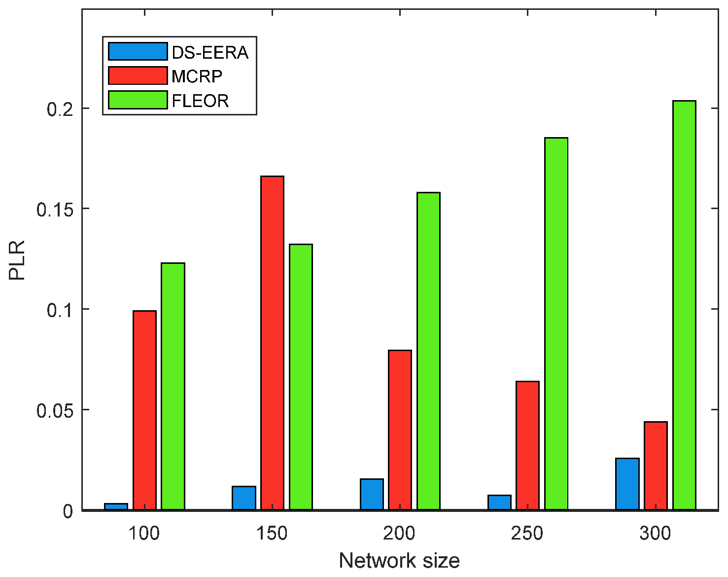
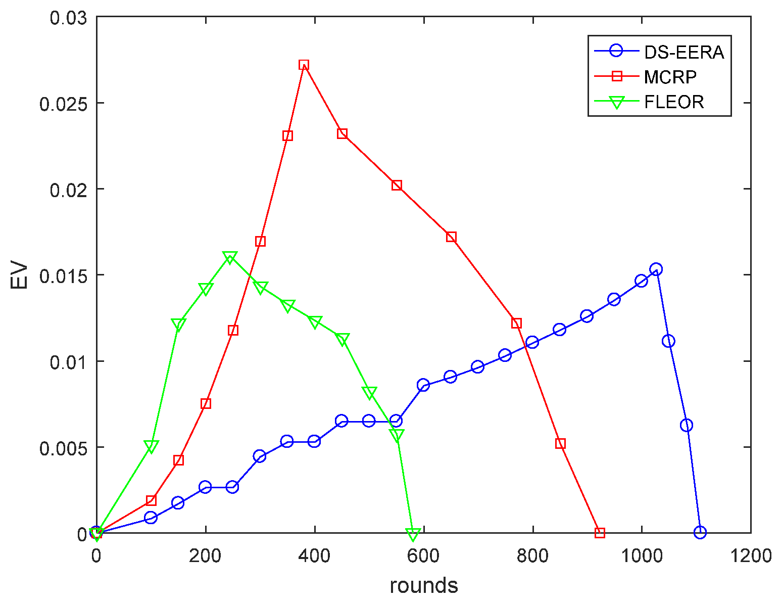
• Significantly, the simulation results show that DS-EERA can not only reduce energy consumption effectively and prolong network lifetime in energy-constrained networks but also achieve lower packet loss rate and increase the reliability of data transmission.

The rest of the paper is organized as follows: Section 2 reviews the related research works. The network model and DS evidence rule are introduced in Section 3. We describe the DS-EERA algorithm in detail in Section 4. The performance of our algorithm is analyzed and discussed according to relevant simulation results in Section 5. Finally, the conclusion is summarized in Section 6.

2. Related Works

Since sensor nodes are mostly powered by batteries, once some nodes are exhausted, the network may not work properly. Therefore, energy-saving has always been one of the keys to the efficient operation of WSN. Some traditional methods mainly reduce the transmission distance and energy consumption of the path, thus prolonging the overall lifetime of the network [9,10]. Authors in [9] select the neighbor node with the fewest hops from the source node to the sink node as the relay, and when there are multiple paths with the fewest hops, the remaining energy of the node is used as the determinant. Ho et al. [10] proposed a ladder diffusion algorithm based on ant colony optimization (ACO) to solve the problem of energy consumption in routing. The algorithm mainly uses the ACO mechanism to determine transmit paths, which effectively reduces energy consumption. In some way, these algorithms based on minimum hop count are equivalent to the minimum energy routing [11]. Although this kind of method can reduce the energy consumption of the path, it has obvious disadvantages of only some nodes undertake the data transmission in a period of time while other nodes are idle. That is to say, when they choose the forwarding node, they do not consider the residual energy, which is very easy to make some nodes run out of energy prematurely and result in uneven energy distribution between nodes. Thus the network lifetime is always at a lower level.

In response to the above problems, in some algorithms for solving load balancing [12,13,14], Zhang D et al. [12] proposed a forward-aware factor-based energy balance routing protocol (FAF-EBRM), which uses the energy density of the forward region and the traffic on the link to alleviate congestion. However, without minimizing the energy consumption of the path, it will lead to energy loss due to detours. For this reason, some algorithms minimize the path energy consumption as much as possible while ensuring the energy balance of nodes [13,14]. The ACOHCM proposed by Ailian J et al. [13] combines the advantages of the ant colony optimization algorithm and minimum hop routing strategy to effectively reduce network energy consumption. The ESRA proposed by Tang L et al. [14] first constructs the minimum energy consumption tree and then propose the “cut edge” strategy to balance the load between nodes, which can effectively utilize the energy and extend the network lifetime. However, the computational complexity and communication overhead required by the two algorithms are large and may consume too many resources in practical applications. Therefore, it is unreasonable to only consider single routing information or adopt a simple mathematical model in routing decisions, and it is also necessary to comprehensively consider various attributes of the network. Among them, the method of multi-attribute decision-making (MADM) can be well applied to routing.

The most widely used multi-attribute decision-making methods include the technique for order preference by similarity to ideal solution (TOPSIS), fuzzy theory and DS evidence theory. In some routing protocols [11,15,16] that use TOPSIS, such as the Multi-criteria based centralities measures routing protocol (MCRP) [15], it is mainly to sort multiple network attribute matrices to obtain the optimal solution. However, the routing decision using the TOPSIS can only reflect the relative closeness of each attribute to its ideal solution, which does not reflect the closeness to the overall ideal solution. In addition, in other algorithms that adopt fuzzy theory for route selection [17,18,19], such as fuzzy-logic-based energy optimized routing (FLEOR) algorithm [18], the determination of attribute weight has a strong subjectivity, that is, the fuzzy rules are determined artificially, and the lack of objectivity may lead to the final decision not be the optimal. The DS evidence theory is simple to calculate and has low demand for prior knowledge. It can use reasonable theoretical derivation to fuse the multi-faceted attributes of the sensor nodes and obtain a good judgment. Meanwhile, DS evidence theory is easy to calculate and has a low demand for prior knowledge. It can use reasonable theoretical derivation to fuse multiple attributes of sensor nodes and get good decision results. However, in WSN, a lot of previous research on DS evidence theory mainly focus on data fusion of nodes to enhance the reliability and security of information acquisition [20,21,22,23,24,25]. Thus the application of attribute fusion in sensor nodes as a routing decision-making method is very few. In the DS-EERA proposed in this paper, based on DS evidence theory, we consider multiple factors affecting energy efficiency and reliability, and then integrate the credibility and fuzzy information of nodes attributes to achieve optimal routing decisions.

3. Network Model and Evidence Theory

3.1. Network Model

The wireless sensor network studied in this paper is mainly used for event discovery and information collection. Due to the limited communication distance between sensor nodes, the nodes usually transmit data to the base station through multi-hops. How to find the path with the least energy consumption from a source node to a sink node is a priority for routing algorithms.

The topology of WSN is shown in Figure 1. The information collection terminals are regarded as common nodes, which transmit the collected data to a sink node through multi-hop forwarding. Suppose in the sensor network with an area of L × L, there are a number of common nodes and a single sink node located in the center, and all nodes are no longer moved after deployment. The location between nodes is determined in [26]. All sensor nodes are isomorphic, with routing, sending and receiving functions, any two nodes can communicate in single-hop or multi-hop, and the initial state is the same. The initial load of the nodes is 0, and the initial energy is $E_0$.

The information exchange method between nodes is as [27]. That is, each node has a unique identifier (ID), which maintains a buffer to store information such as residual energy, packet ID, next-hop ID, sender IDs etc. This information is updated in real-time as the forward neighbor changes. It is noted that the traffic queue length of the nodes is limited, and the data packet is processed in first-in first-out (FIFO) mode.

To more clearly describe the algorithm, this paper makes the related definitions as follows:

Definition 1. 

Network lifetime: network lifetime is defined as the round number when the first dead node appears due to the energy exhaustion.

Definition 2. 

Forward neighbor node set: In order to avoid data backhaul, it is necessary to ensure that data is forwarded in the direction of the sink node. The forward neighbor node set includes the neighbor nodes in the forward semicircle region of node$i$within maximum communication radius R. Based on the nodes spatial relationship in Figure 1 and forward transmission model in [12], the forward neighbor node set is defined as follows:

$$FN(i)=\left\{a\right|d_{ia}\le R,d_{as}<d_{is}\}.$$

(1)

where node$a$is any forward neighbor node of node$i$, $d_{ia}$is the distance from node i to node$a$, $d_{as}$and$d_{is}$are the distances from node i and node$a$to the sink node respectively, R is the maximum communication radius of node i.

Definition 3. 

Forward energy consumption: for any node$a\in FN(i)$, the energy consumption during the communication between node$a$and sink node is the forward energy consumption which denoted as$e_{as}.$

Definition 4. 

Candidate node set: for any node i, the candidate node set$C{N}_{next}(i)$is the nodes in$FN(i)$that satisfy the criterion in Algorithm 1, which will be detailed in Section 4.

In the WSN routing decision, the selection of the next hop is affected by the environment and the performance of a node (such as energy status and queue length). The optimal routings determined under different attribute indexes are different and even conflict. As a classical multi-attribute decision-making method, DS evidence theory can effectively deal with uncertain and incomplete information, which can provide a theoretical basis and fusion rules for the comprehensive judgment of sensor node performance. The following will introduce the fusion rules of DS evidence theory.

3.2. DS Evidence Theory

DS evidence theory was put forward by Dempster and Shafer in the 1970s, and it can be used in information fusion and uncertainty inference. It establishes a one-to-one correspondence between the proposition and set, which has been successfully applied in data fusion, intelligent optimization, fault diagnosis, decision analysis etc. [28].

This paper mainly adopts the basic probability assignment (BPA) function and DS evidence fusion rule, which is described below.

(1) Basic probability assignment function

The frame of discernment Θ is defined as a set of all possible values of the proposition A, $m(A)$ is the basic probability assignment (BPA) function on the frame of discernment $\Theta$, that is the degree of support in proposition $A$. If $A_{\partial }\in \Theta$, $m(A_{\partial })>0$, then $A_{\partial }$ called focal element [29]. The BPA function satisfies the following demands:

$$\{\begin{array}{l}m(\Phi )=0 ,\Phi is null\\ {\displaystyle \sum _{\partial =1}^{n}m(A_{\partial })}=1\end{array}$$

(2)

(2) DS evidence fusion rules

Suppose $m_1$ and $m_2$ are two BPA functions over the same frame of discernment $\Theta$, and the focal elements are included in $A=\{A_1,A_2,\dots ,A_k\}$. Then the orthogonal sum of these two evidences $m_1$ and $m_2$ is:

$$m(A)=(m_1\oplus m_2)(A)\begin{array}{c}=\{\begin{array}{c}0 ,A=\Phi \\ \frac{{\displaystyle \sum _{A_{\partial }\cap A_{\beta }\ne \Phi }{m}_1(A_{\partial })m_2(A_{\beta })}}{(1-K)},A\ne \Phi ,A\subset \Theta \end{array}\end{array}$$

(3)

where $1\le \partial ,\beta \le k$, $K={\displaystyle \sum _{A_{\partial }\cap A_{\beta }=\Phi }}{m}_1(A_{\partial })m_2(A_{\beta })$, $A_{\partial }\cap A_{\beta }=\Phi$ denotes proposition $A_{\partial }$ and $A_{\beta }$ are completely in conflict.

The above is an example of two evidences. When more than two evidences are needed as decision-making indexes, we fuse the first two evidences according to Equations (2) and (3), and then fuse the result as new evidence with the third evidence, so as to get the final fusion result by analogy.

4. DS-EERA

In this paper, the DS evidence theory is applied to WSN routing decision-making. For each sensor node, the factors such as residual energy, the shortest path to the sink node, node traffic, energy density of neighboring nodes and the forward distance are taken into account when selecting the next hop. Thus, the above factors are abstracted into three indexes: “transmission energy efficiency ratio”, “idleness degree” and “energy density factor”, which can be regarded as three evidences. Based on the above three indexes and triangular membership function, we establish the basic probability assignment (BPA) function, and the reliability of the node belonging to each membership function can be obtained. Then, the entropy weight method is used to objectively weigh the relative importance of each index in routing decision-making. Finally, the neighbor node with the best fusion result will be selected as the next hop. This section introduces the DS-EERA in detail and focuses on the establishment of attribute indexes, the weight distribution of each index and the routing selection.

4.1. Attribute Indexes

(1) Transmission energy efficiency ratio

This paper considers the spatial positional relationship between the current node $i$, the forward neighbor node $a$ and the sink node, as well as the energy status of each node to establish a data transmission path that reduces energy consumption and delay. The closer the forward neighbor node of node i is to the sink node, and the closer the straight-line distance $d_{is}$ is, the fewer hops it forwards along the path, the faster the data can be transmitted to the sink node. As can be seen from Figure 1, node $a$ is closer to the sink than node $b$ and closer to a straight line $d_{is}$ than node $c$, so node i under this index will prefer node $a$ as the next hop node. At the same time, from the perspective of residual energy, when residual energy $E_i$ is small, it is hoped that the smaller the energy consumption $e_{ia}$ is, the forward distance $d_{as}$ is as large as possible, and node $a$ can bear more forward energy consumption $e_{as}$. On the contrary, when the residual energy $E_i$ is relatively abundant, and the residual energy $E_a$ of the forward neighbor node $a$ is generally small, it is hoped that node $i$ can share more transmission energy consumption as large as possible. Based on the above two aspects, the transmission energy efficiency ratio is established to reflect the ability of nodes to balance energy utilization in data transmission. Its expression is as follows:

$$p(a)=\frac{d_{is}}{d_{ia}+d_{as}}·(\frac{e_{as}}{E_i}+\frac{e_{ia}}{E_a})$$

(4)

Normalize $p(a)$ for unified dimension:

$$P(a)=\frac{p(a)}{\max \{p(a)\}}$$

(5)

where $P(a)$ is a benefit index, the larger $P(a)$ is, the more efficient it is to utilize energy so that the data is forwarded along the shortest path as much as possible.

(2) Idleness degree

Considering the transmission energy efficiency ratio, the data can be forwarded along the path with the highest energy efficiency ratio. However, due to the uneven distribution of nodes in the wireless sensor network and bursts of data streams, some nodes in the forwarding path, especially those near the sink node, are prone to packet loss due to the excessive data forwarding tasks. The amount of data exceeds the size of the cache area, seriously affecting the Quality of Service (QoS). Therefore, from the perspective of balanced traffic, the idleness degree is defined as follows:

$$C_{idle}(a)=1-\frac{Q_c^a+Q_{in}^a-Q_{out}^a}{Q_{\max }}$$

(6)

where $Q_c^a$ is the current data traffic of the node $a$, $Q_{in}^a$ is the data traffic of the inflow node $a$, $Q_{out}^a$ is the data traffic of the outflow node $a$ and $Q_{\max }$ is the maximum length of the buffer. $C_{idle}(a)$ can reflect the ability of the node to accommodate the amount of data, it is a benefit index. Thus, the larger $C_{idle}(a)$, the more data the node $a$ is able to receive.

(3) Energy density factor

In the next hop selection process, in order to balance the network energy, the data should be transmitted to the forward neighbor nodes with more residual energy as much as possible. At the same time, the energy state around the next hop node should be considered to avoid transmitting to the energy empty area. For this purpose, the index of energy density factor of node $a$ is established, and the expression is as follows:

$$J(a)=\frac{E_a}{E_o}·\frac{1}{0.5\pi l^2}\left(\sum _{a\in FN(i),t\in FN(a)}{E}_t\right)$$

(7)

where $l$ is the max distance between node $i$ and the nodes of $FN(i)$. The energy density factor $J(a)$ is benefit index, that is, the larger $J(a)$ is, and the higher residual energy and energy density node will be preferred when choosing the next hop.

4.2. Weight Assignment

The entropy weight method is used to determine the index weight by the amount of information provided by the entropy value of each index [30]. The size of the entropy weight is directly related to the evaluated object. From the perspective of information, entropy weight indicates how much information the index contributes to the problem, i.e., the greater the difference within the index value, the greater the corresponding index information, the more important the index is. In this paper, the entropy weight method is used to determine the weight of each index, which is divided into the following steps:

(1) Standardized decision matrix

For any node $i$, suppose its forward neighbor node to be the evaluation object set $M=(M_1,M_2,\dots ,M_m)$, the set of three indexes in this paper is $D=(D_1,D_2,D_3)$, and the value of the evaluation object $M_a$ in index $D_b$ is denoted as $x_{ab}(a=1,2,\dots ,m ;b=1,2,3)$, then the decision matrix $X$ is established as follows:

$$X=\left(\begin{array}{l}{\mathrm{x}}_{11}{ \mathrm{x}}_{12}{ \mathrm{x}}_{13}\\ {\mathrm{x}}_{21}{ \mathrm{x}}_{22}{ \mathrm{x}}_{23}\\ ⋮ ⋮ ⋮\\ {\mathrm{x}}_{m1}{ \mathrm{x}}_{m2}{ \mathrm{x}}_{m3}\end{array}\right)$$

(8)

In order to eliminate the different dimensions of each index, the standardized decision matrix $V={[v_{ab}]}_{m\times 3}$ is obtained. According to the index property [31], the indexes that we established are all benefit indexes, i.e., the larger the index value is, the better the performance is. It is normalized as follows:

$$v_{ab}=\frac{x_{ab}-\min x_b}{\max x_b-\min x_b}$$

(9)

(2) Characteristic weight of evaluation object $a$ under index $b$

In this paper, sensor nodes are used as an evaluation object. The smaller the entropy value is, the greater the weight is, i.e., the larger the information content of the corresponding evaluation index is, the more important the index is. According to the definition of relative entropy [32], the increase of information means the decrease of entropy value, so entropy can be used to measure the size of this information.

The characteristic weight of node $a$ under index $b$ is:

$${\theta }_{ab}=\frac{v_{ab}}{{\displaystyle \sum _{a=1}^m{v}_{ab}}},0<a\le m , 0<b\le 3$$

(10)

Thus, obtain the entropy value $E{N}_b$ of index $b$:

$$E{N}_b=-\frac{1}{\ln m}{\displaystyle \sum _{a=1}^m{\theta }_{ab}\ln {\theta }_{ab}}$$

(11)

(3) The entropy weight of each index

It can be known from Equations (10) and (11) that for a certain index, the greater the difference of $v_{ab}$, the smaller $E{N}_b$ is i.e., the larger the amount of information reflected by this index, the more weight should be given, thus the entropy weight of index $b$ is defined as follows:

$$w_b=\frac{1}{1-\frac{E{N}_b}{{\displaystyle \sum _{b=1}^3(1-E{N}_b)}} }$$

(12)

4.3. BPA Function Based on Triangular Membership Function

In this paper, the frame of discernment $\Theta$ includes “next hop”, “non-next hop” and “fuzzy”, which is described as $A=\{A_1,A_2,A_3\}$ under the three indexes. The three attribute indexes represent three kinds of evidence respectively, i.e., $m_1$ (transmission energy efficiency ratio), $m_2$ (idleness degree) and $m_3$ (energy density factor).

Because all three attribute indexes are benefit type, the BPA function can be established based on the same triangular membership function (shown in Figure 2). In Figure 2, $G_1$ is the membership of the forward neighbor node belonging to “next hop”, $G_2$ is the membership belonging to “non-next hop”, and $G_3$ is the membership belonging to “fuzzy”. Once obtain the index value of node $a$ under any three indexes $P(a) , C_{idle}(a) , J(a)$, the membership degree of the next hop, non-next hop and fuzzy can be obtained according to $G_1$,$G_2$,$G_3$ respectively. The three membership functions are established as follows:

$$G_1(g(a))=\{\begin{array}{c}0 0<g(a)\le g_{\min }\\ \frac{g(a)-g_{\min }}{g_{\max }-g_{\min }} g_{\min }<g(a)\le g_{\max } \\ 1 g_{\max }<g(a)\le 1\end{array}$$

(13)

$$G_2(g(a))=\{\begin{array}{c}1 0< g\left(a\right)\le g_{\min }\\ \frac{g(a)-g_{\max }}{g_{\min }-g_{\max }} g_{\min }<g(a)\le g_{\max }\\ 0 g_{\max }<g(a)\le 1\end{array}$$

(14)

$$G_3(g(a))=\{\begin{array}{c}\begin{array}{l}1-\frac{|g(a)-\frac{g_{\min }+g_{\max }}{2}|}{\frac{g_{\max }-g_{\min }}{2}}, |g\left(\mathrm{a}\right)-\frac{(g_{\min }+g_{\max })}{2}|\le \frac{g_{\max }-g_{\min }}{2} \end{array}\\ 0 , |g(a)-\frac{(g_{\min }+g_{\max })}{2}|\ge \frac{g_{\max }-g_{\min }}{2}\end{array}$$

(15)

where $g(a)$ can represent any three attribute indexes $P(a)$, $C_{idle}(a)$, $J(a)$.$g_{\min }$ and $g_{\max }$ are the minimum and maximum values of each index.

As can be seen from Figure 2, when $g(a)<g_{\min }$, the membership degree of the node $a$ selected as the next hop is 0, i.e., under this index, the probability that the node $a$ is selected as the next hop is 0. When $g(a)>g_{\max }$, the probability that node $a$ is selected as the next hop under this index is 1.

After the membership function of each index is obtained in the above, the value of the membership function determines the possibility that the node belongs to the corresponding category. Then the membership function is normalized as the BPA function, and BPA values of next hop, non-next hop and fuzzy can be obtained. Furthermore, the weight of the index in Equation (12) is combined with the corresponding BPA value. The larger the weight of an index, the more important the index is when selecting the next hop. Thus, the BPA function of the forward neighbor node $a$ of any node $i$ under attribute $b$ shown as follows:

$$m_b(A_t^a)=\frac{w_b\cdot G_t(g(a))}{{\displaystyle \sum _{t=1}^3{w}_b\cdot G_t(g(a))}} b=1,2,3;t=1,2,3$$

(16)

4.4. Fusion of Attribute Indexes and Routing Decision

Based on the data fusion rule of DS evidence theory [24,33], firstly, the BPA value of transmission energy efficiency ratio ($m_1(A_{\partial }^a)$) and idleness degree ($m_2(A_{\beta }^a)$) of the node $a$ are fused based on Equation (16) as follows:

$$m(A^a)=(m_1\oplus m_2)(A^a)\begin{array}{c}=\{\begin{array}{c}\hspace{1em}0\hspace{1em}\hspace{1em}\hspace{1em}\hspace{1em}\hspace{1em}\hspace{1em}\hspace{1em}\hspace{1em}\hspace{1em},A=\Phi \\ \frac{{\displaystyle \sum _{A_{\partial }\cap A_{\beta }\ne \Phi }\{m_1(A_{\partial }^a)m_2(A_{\beta }^a)\}}}{1-K},A\ne \Phi ,A\subset \Theta \end{array}\end{array}$$

(17)

where $K={\displaystyle \sum _{\Phi =A_{\partial }\cap A_{\beta }}}{m}_1(A_{\partial }^a)m_2(A_{\beta }^a)$, $\partial =1,2,3$, $\beta =1,2,3$, $\Theta =\{A_1,A_2,A_3\}$, $A_1$ is “next hop”, $A_2$ is “non-next hop”, and $A_3$ is “fuzzy”.

In our paper, it should be noted that $m(A_1^a)$ and $m(A_2^a)$ are calculated by the Equation (17), but $m(A_3^a)$ is calculated as follows:

$$m(A_3^a)=1-m(A_1^a)-m(A_2^a)$$

(18)

At this point, the BPA value corresponding to each focal element of the first fusion result can be obtained. After obtaining the fusion result $m(A^a)$ of the first two BPA value of $m_1(A_{\partial }^a)$ and $m_2(A_{\beta }^a)$, $m(A^a)$ is equivalent to a BPA function of new evidence, which will be fused with the remaining BPA function $m_3(A^a)$ (energy density factor) by the same DS fusion rule. The value of fusion results $m{(A_1^a)}_{final}$, $m{(A_2^a)}_{final}$ and $m{(A_3^a)}_{final}$ can also be obtained by the above fusion rules.

To more clearly describe the routing process of node i to its forward neighbor nodes, the routing Algorithm 1 is described as follows:

Algorithm 1 The Next Hop Selection

Input: Node $i$, index weight $w_b$, transmission energy efficiency ratio $P(a)$, idleness degree $C_{idle}(a)$, energy density factor $J(a)$, the triangle membership function model $G$. Output: The next hop $j$ 1:   for  $a=1:m$    //$m$ is the number of forward neighbor nodes of node i 2:             j = 1, $C{N}_{next}(i)\leftarrow \Phi$ 3:         According to G, traverse m: 4:                 $g(a)\leftarrow P(a),g(a)\leftarrow C_{idle}(a),g(a)\leftarrow J(a)$, 5:                 find $g_{\max }\leftarrow \max \{g(a)\}$, $g_{\min }\leftarrow \min \{g(a)\}$, 6:         Establish triangular membership function $G_t(g(a))$ 7:         Combine $G_t(g(a))$ and corresponding weight to establish BPA function: 8:                 $m_b(A_t^a)\leftarrow G(g(a)),w_b$ 9:         Fuse the three indexes by Equations (17) and (18): 10:                 $m(A_t^a)\leftarrow$$m_1(A_t^a)$,$m_2(A_t^a)$; $m{(A_t^a)}_{final}\leftarrow$$m_3(A_t^a)$,$m(A_t^a)$ 11:       if   $m(A_1^a)>m(A_2^a)\&m(A_1^a)>m(A_3^a)$     //criterion 12:                 $C{N}_{next}(i)\leftarrow C{N}_{next}(i)+a$ 13:       end if 14: end for 15:               $j\leftarrow \max (m{(A_1^a)}_{final}),a\in (C{N}_{next}(i))$ 16: Return j

The following is a fused example of any two forward neighbor nodes $a_1$ and $a_2$ of node i according to Algorithm 1. In

Table 1. The routing decision result.

FN(i)	Indexes	Next Hop t = 1	Non-Next Hop t = 2	Fuzzy t = 3
	$m_1\left(A_t^{a_1}\right)$	0.0025	0.9900	0.0075
a1	$m_2\left(A_t^{a_1}\right)$	0.3775	0.2055	0.4170
	$m_3\left(A_t^{a_1}\right)$	0.0099	0.9900	0.0001
Fusion results	$m{\left(A_t^{a_1}\right)}_{final}$	0.00999625	0.9900	0.00000375
	$m_1\left(A_t^{a_2}\right)$	0.9666	0.0110	0.0224
a2	$m_2\left(A_t^{a_2}\right)$	0.8125	0.0624	0.1251
	$m_3\left(A_t^{a_2}\right)$	0.2307	0.3077	0.4616
Fusion results	$m{\left(A_t^{a_2}\right)}_{final}$	0.9924	0.0055	0.0021

, node $a_1$ is obviously judged as “non-next hop” under the indexes of transmission energy efficiency ratio and energy density factor, and is judged as “fuzzy” under idleness degree. According to DS evidence fusion rule, the fusion result is $m{(A_2^{a_1})}_{final}>m{(A_1^{a_1})}_{final}>m{(A_3^{a_1})}_{final}$, where $m{(A_2^{a_1})}_{final}$ is the largest, and thus node $a_1$ is judged as “non-next hop”, not included in candidate neighbor set $C{N}_{next}(i)$. For node $a_2$, the fusion result satisfies the criterion and thus belongs to the $C{N}_{next}(i)$. By analogy, the fusion results of all forward neighbor nodes of node i can be calculated, and then the fusion results in $C{N}_{next}(i)$ will be sorted. The node with largest $m{(A_1^a)}_{final}$ in $C{N}_{next}(i)$ will be selected as the next hop of node i. At this point, the next hop of each node and routing path in this round will be determined. The network performs DS-EERA as described above until the network lifetime is reached.

5. Simulation Results and Analysis

In this section, the proposed algorithm is verified by a large number of simulation experiments in MATLAB, and compared with two multi-attribute algorithms: TOPSIS based MCRP algorithm and fuzzy theory based FLEOR algorithm. In order to avoid the contingency of the experimental results, all sensor nodes of different network size (i.e., number of sensor nodes) randomly distributed in the monitoring area, and take the average of the experimental results. The specific simulation parameters are shown in

Table 2. Simulation parameters.

Definition	Value
Simulation area (L × L)	100 × 100 m2
Network size (N)	100~300
Sink	(50, 50)
Maximum communication radius (R)	30 m
Packets size	1024 bits
Buffer size	20 packets
Initial energy (E0)	0.5 J
Data generation rate	1024 bits/round
Energy consumed in electronics (Eelec)	50 nJ/bit
Amplifier energy dissipation in free space (Efs)	10 pJ/bit/m2
Amplifier energy dissipation in multipath (Emp)	0.0013 pJ/bit/m4
Energy consumed in data aggregation (EDA)	5 nJ/bit/signal
Distance threshold (dth)	87 m

.

In this model, both the multipath fading and free space channel models are taken into account [34,35]. All the simulation parameters are not constant. We can change some parameters according to different scenarios.

5.1. Average Packet Loss Rate

The packet loss rate (PLR) can reflect the advantages and disadvantages of the network in congestion avoidance. Figure 3 shows the comparison of the packet loss rate with the change of network size under different algorithms. It can be seen that compared with the other two algorithms, the packet loss rate of DS-EERA in this paper is always stable at a lower value with the change of network size. This is because both the MCRP and the FLEOR do not consider the queue length of the nodes when routing, and a large amount of data is concentrated in some “hot spots” areas at the same time, resulting in the nodes exceeding their own load capacity due to too much received data. Thus a large amount of data is discarded. Our algorithm adopts “idleness degree” as one of the attribute indexes of decision making, and uses the entropy weight method to periodically adjust the importance of each index according to the network operation, ensuring that the node selects the forward neighbor node with large idleness to become the next hop. It is more likely to be able to effectively alleviate congestion and make network traffic more balanced.

5.2. Energy Efficiency

In WSN with limited energy, one of the key tasks is to improve energy utilization, i.e., to maximize the network lifetime with limited energy. Energy variance (EV) can reflect the difference of residual energy of each node. The smaller the value and the smaller the curve fluctuation, the more balanced the energy of the network. The residual energy reflects the energy distribution of all nodes in the network when the first node dies. The more balanced the residual energy, the greater the energy efficiency of the network and the longer the network lifetime.

From Figure 4, we note that the volatility of the EV curve of DS-EERA is smaller than that of the other two algorithms, and the energy distribution between nodes is more balanced. Obviously, the network lifetime of the DS-EERA is 1027 rounds, which are 311% and 170% of the FLEOR and MCRP respectively. This is because DS-EERA considers the “energy density factor” of the forward neighbor nodes when routing, and avoids the data being transmitted to the energy hole region, so that the energy of each node is evenly distributed. Meanwhile, the three EV curves increase with the number of network rounds. When the first node dies (i.e., network lifetime), EV reaches the maximum and then decreases to 0 with the death of the nodes in the network. At the same time, it can be seen that from the comparison of Figure 5a–c, when the first node dies in the network, the most nodes of energy in DS-EERA algorithm is less than 25%, and the energy of most nodes in MRCP and FLEOR algorithm is between 75% and 100%, indicating that the DS-EERA algorithm in this paper can make full use of energy and has a high energy efficiency.

In addition, from the number of death rounds in the first node of the network, the network lifetime of the DS-EERA is 170% and 310% longer than the MCRP and FLEOR respectively, which means that the network can maintain a longer effective working time. At the same time, when the nodes of MCRP and FLEOR all die, DS-EERA has not yet seen the death of the first node, showing the good performance of our algorithm.

5.3. Average Number of Hops and Average Energy Consumption

(1) Average number of hops

To some extent, the average number of hops (ANH) can qualitatively reflect the data transmission delay in the network, that is, the smaller the average hops is, the faster the data can be transmitted to the sink node. Figure 6 is a comparison of the average hops of the three algorithms. It can be seen that, with the increase of the network size, the ANH curve has an upward trend, but DS-EERA remains the lowest, this is because the “energy transmission ratio” of the algorithm in this paper considers the shortest path as much as possible, so as to reduce the number of hops. At the same time, the “idleness degree” index considers the time of packet queuing and processing, and the combination of the two can effectively reduce the delay.

(2) Average energy consumption

The average energy consumption (AEC) represents the average energy consumption of all nodes in each data transmission round, which is used to measure the energy consumption rate of the network. Figure 7 is a comparison of average energy consumption using different algorithms, as can be seen from that, the DS-EERA in this paper has the lowest average energy consumption and can effectively balance the energy utilization, so its network lifetime is also the highest (Figure 4). The AEC and EV of MCRP and FLEOR algorithms are large, so the energy utilization is insufficient, resulting in lower network lifetime.

6. Conclusions

In order to improve the energy efficiency and the reliability of the whole network, this paper innovatively applies the data fusion rules of DS evidence theory to WSN routing decision-making and proposes an energy-efficient and reliable-routing algorithm based on weighted DS evidence theory. For each node in the network, three attribute indexes are established: transmission energy efficiency ratio, idleness degree and energy density factor, and the entropy weight method is adopted to dynamically determine the weight of each index, and the combination of the above two can get the BPA function. Then the DS evidence fusion rule is used to fuse the reliability value of the index in turn, which can objectively make the optimal routing decision. The simulation results show that, compared with MCRP and FLEOR algorithm, DS-EERA can effectively reduce network energy consumption, prolong the network lifetime and also improve packets loss rate, showing a good performance in transmission reliability.

In future work, we will focus on combining mobile charging technology and routing optimization strategies to enhance the performance of wireless sensor networks.

References

1. Alhmiedat, T.; Taleb, A.A.; Bsoul, M. A Study on Threads Detection and Tracking Systems for Military Applications using WSNs. IJCA 2012, 40, 12–18. [Google Scholar]
2. Mathur, P.; Nielsen, R.H.; Prasad, N.R.; Prasad, R. Cost Benefit Analysis of Utilizing Mobile Nodes in Wireless Sensor Networks. Wirel. Pers. Commun. 2015, 83, 2333–2346. [Google Scholar]
3. Shen, J.; Wang, J.; Zhang, J.; Wang, S. Location-Aware Routing Protocol for Underwater Sensor Networks; Springer: Dordrecht, The Netherlands, 2013; pp. 609–617. [Google Scholar]
4. Chen, S.; Lai, C.; Huang, Y.; Jeng, Y. Intelligent home-appliance recognition over IoT cloud network. In Proceedings of the 2013 9th International Wireless Communications and Mobile Computing Conference (IWCMC), Sardinia, Italy, 1–5 July 2013. [Google Scholar]
5. Yan, J.; Zhou, M.; Ding, Z. Recent Advances in Energy-efficient Routing Protocols for Wireless Sensor Networks. IEEE Access 2016, 4, 5673–5686. [Google Scholar]
6. Sergiou, C.; Vassiliou, V. Alternative path creation vs. data rate reduction for congestion mitigation in wireless sensor networks. In Proceedings of the 9th ACM/IEEE International Conference on Information Processing in Sensor Networks, Stockholm, Sweden, 12–16 April 2010. [Google Scholar]
7. Demura, K.; Seto, A.; Sasaki, J. The forecasting an importation liberalization effect on the regional agriculture caused by the GATT Uruguay round: Simulation analysis using input-output in a macro model framework. Sensors 2017, 52, 15–27. [Google Scholar]
8. Li, Y.; Shen, B.; Zhang, J.; Gan, X. Offloading in HCNs: Congestion-Aware Network Selection and User Incentive Design. IEEE Trans Wirel. Commun. 2017, 16, 6479–6492. [Google Scholar]
9. Chiang, S.; Huang, C.; Chang, K. A Minimum Hop Routing Protocol for Home Security Systems Using Wireless Sensor Networks; IEEE Press: New York, NY, USA, 2007; Volume 53, pp. 1483–1489. ISBN 1558–4127. [Google Scholar]
10. Ho, J.; Shih, H.; Liao, B.; Chu, S. A ladder diffusion algorithm using ant colony optimization for wireless sensor networks. Inf. Sci. 2012, 192, 204–212. [Google Scholar]
11. Suh, Y.; Kim, K.; Shin, D.; Youn, H. Traffic-Aware Energy Efficient Routing (TEER) Using Multi-Criteria Decision Making for Wireless Sensor Network. In Proceedings of the 2015 5th International Conference on IT Convergence and Security (ICITCS), Kuala Lumpur, Malaysia, 24–27 August 2015. [Google Scholar]
12. Zhang, D.; Li, G.; Zheng, K. An Energy-Balanced Routing Method Based on Forward-Aware Factor for Wireless Sensor Networks. IEEE Trans Ind. Inform. 2013, 10, 766–773. [Google Scholar]
13. Ailian, J.; Lihong, Z. An Effective Hybrid Routing Algorithm in WSN: Ant Colony Optimization in combination with Hop Count Minimization. Sensors 2018, 18, 1020. [Google Scholar]
14. Tang, L.; Lu, Z.; Cai, J.; Yan, J. An Equilibrium Strategy-Based Routing Optimization Algorithm for Wireless Sensor Networks. Sensors 2018, 18, 3477. [Google Scholar]
15. Hajji, F.E.; Leghris, C.; Douzi, K. Adaptive Routing Protocol for Lifetime Maximization in Multi-Constraint Wireless Sensor Networks. J. Commun. Inf. Netw. 2018, 3, 67–83. [Google Scholar]
16. Wang, X.; Li, D.; Zhang, X.; Cao, Y. MCDM-ECP: Multi Criteria Decision Making Method for Emergency Communication Protocol in Disaster Area Wireless Network. Appl. Sci. 2018, 8, 1165. [Google Scholar]
17. Khan, B.M.; Bilal, R.; Young, R. Fuzzy-TOPSIS Based Cluster Head Selection in Mobile Wireless Sensor Networks. J. Electr. Syst. Inf. Technol. 2017, 5, 928–943. [Google Scholar]
18. Jiang, H.; Sun, Y.; Sun, R.; Xu, H. Fuzzy-Logic-Based Energy Optimized Routing for Wireless Sensor Networks. Int. J. Distrib. Sens. Netw. (IJDSN) 2013, 9, 264–273. [Google Scholar]
19. Shah, B.; Iqbal, F.; Abbas, A.; Kim, K. Fuzzy Logic-Based Guaranteed Lifetime Protocol for Real-Time Wireless Sensor Networks. Sensors 2015, 15, 20373–20391. [Google Scholar]
20. Sun, Z.; Zhang, Z.; Xiao, C.; Qu, G. D-S Evidence Theory Based Trust Ant Colony Routing in WSN. China Commun. 2018, 3, 27–41. [Google Scholar]
21. Aitsaadi, N.; Aitsaadi, N.; Aitsaadi, N.; Oukhellou, L. Fusion-based surveillance WSN deployment using Dempster-Shafer theory. J. Netw. Comput. Appl. 2016, 64, 154–166. [Google Scholar]
22. Yang, K.; Liu, S.; Li, X.; Wang, X. D-S Evidence Theory Based Trust Detection Scheme in Wireless Sensor Networks. Int. J. Technol. Hum. Interact. 2016, 12, 48–59. [Google Scholar]
23. Sun, Z.; Wei, M.; Zhang, Z. Secure Routing Protocol based on Multi-objective Ant-colony-optimization for wireless sensor networks. Appl. Soft Comput. 2019, 77, 366–375. [Google Scholar]
24. Chen, B.; Tao, X.; Yang, M.; Yu, C.; Pan, W. A Saliency Map Fusion Method Based on Weighted DS Evidence Theory. IEEE Access 2018, 6, 27346–27355. [Google Scholar]
25. Fang, Y.; Jie, C.; Yuan, T. A Robust DS Combination Method Based on Evidence Correction and Conflict Redistribution. J. Sens. 2018, 2018, 1–12. [Google Scholar]
26. Lv, Y.H.; Liu, Y.; Hua, J.F. A Study on the Application of WSN Positioning Technology to Unattended Areas. IEEE Access 2019, 7, 38085–38099. [Google Scholar]
27. Ahmed, A.; Bakar, K.A.; Channa, M.I.; Haseeb, K.; Khan, A.W. TERP: A Trust and Energy Aware Routing Protocol for Wireless Sensor Network. IEEE Sens. J. 2015, 15, 1. [Google Scholar]
28. Wang, Y.; Cheng, S.; Zhou, Y.; Peng, G.; Zhou, D.; Chao, C. Decision of air-to-air operation mode of airborne fire control radar based on DS evidence theory. Mod. Radar 2017, 39, 79–84. [Google Scholar]
29. An, J.; Hu, M.; Fu, L.; Jan, J. A Novel Fuzzy Approach for Combining Uncertain Conflict Evidences in the Dempster-Shafer Theory. IEEE Access 2019, 7, 7481–7501. [Google Scholar]
30. Ni, N.; Zhang, S.; Chen, X.; Zhang, X. Audit risk assessment based on entropy weight method and fuzzy analytic hierarchy process. Software 2018, 39, 254–259. [Google Scholar]
31. Zhang, S.; Zhang, M.; Chi, G. Science and technology evaluation model and empirical research based on entropy weight method. J. Manag. 2010, 7, 34–42. [Google Scholar]
32. Li, Y.; Gao, J.; Yu, Y.; Cao, T. An energy-based weight selection algorithm of monitor node in MANETs. In Proceedings of the 2017 International Conference on Computer, Information and Telecommunication Systems (CITS), Dalian, China, 21–23 July 2017. [Google Scholar]
33. Shafer, G.A. A Mathematical Theory of Evidence; Princeton University Press: Princeton, NJ, USA, 1976. [Google Scholar]
34. Kumar, N.; Vidyarthi, D.P. A Green Routing Algorithm for IoT-Enabled Software Defined Wireless Sensor Network. IEEE Sens. J. 2018, 18, 9449–9460. [Google Scholar]
35. Yuan, Y.; Liu, W.; Wang, T.; Deng, Q.G.; Liu, A.F.; Song, H.B. Compressive Sensing-Based Clustering Joint Annular Routing Data Gathering Scheme for Wireless Sensor Networks. IEEE Access 2019, 7, 114639–114658. [Google Scholar]
Figure 1. The topology of the wireless sensor network (WSN).
Applsci 10 01885 g001
Figure 2. Membership function curve under each index.
Applsci 10 01885 g002
Figure 3. The packet loss rate (PLR) comparisons with varying network size.
Applsci 10 01885 g003
Figure 4. The energy variance (EV) comparisons with varying rounds.
Applsci 10 01885 g004
Figure 5. The residual energy distribution of three algorithms when the first node dies are: (a) Residual energy distribution of DS-EERA; (b) residual energy distribution of MCRP; (c) residual energy distribution of FLEOR. Among them, the red nodes indicate that the residual energy percentage is [0, 25%], the yellow nodes indicate that the residual energy is [25%, 50%], the blue nodes indicate that the residual energy is [50%, 75%] and the green nodes indicate that the residual energy is [75%, 100%].
Applsci 10 01885 g005
Figure 6. The average number of hops (ANH) comparisons with varying network size.
Applsci 10 01885 g006
Figure 7. The average energy consumption (AEC) comparisons with varying network size.
Applsci 10 01885 g007