Systematic Quantification of Cell Confluence in Human Normal Oral Fibroblasts

 ,
,  , , and
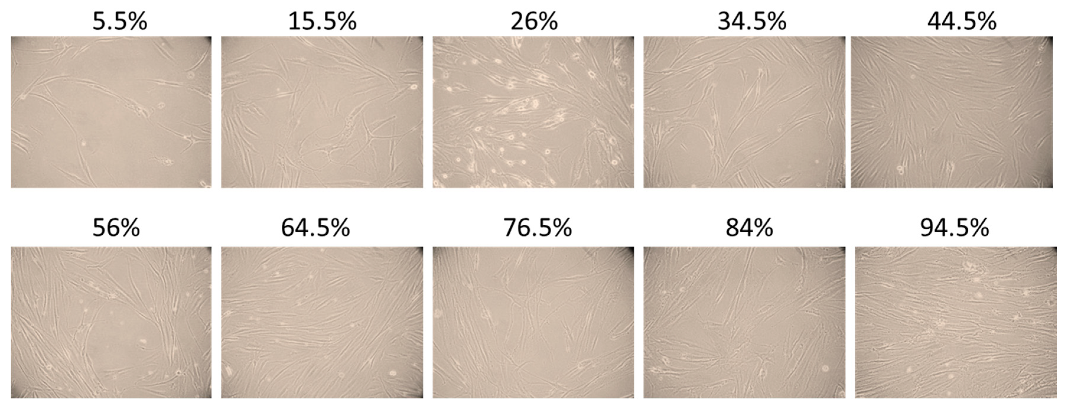
Abstract
:1. Introduction
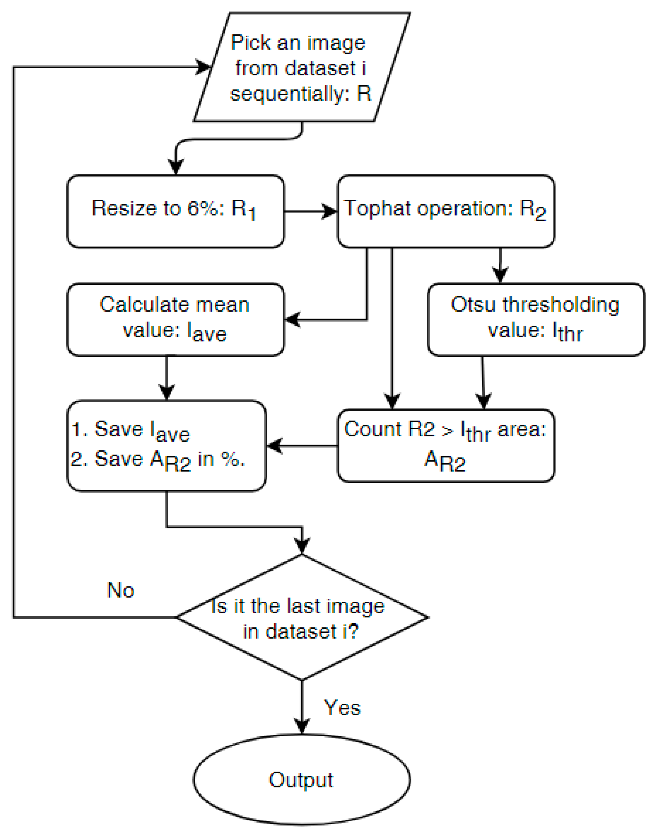
2. Materials and Methods
- (1)
- The illumination setting of the digital camera should be consistent;
- (2)
- The camera parameters such as the focal length and zoom factor should be fixed.
3. Results
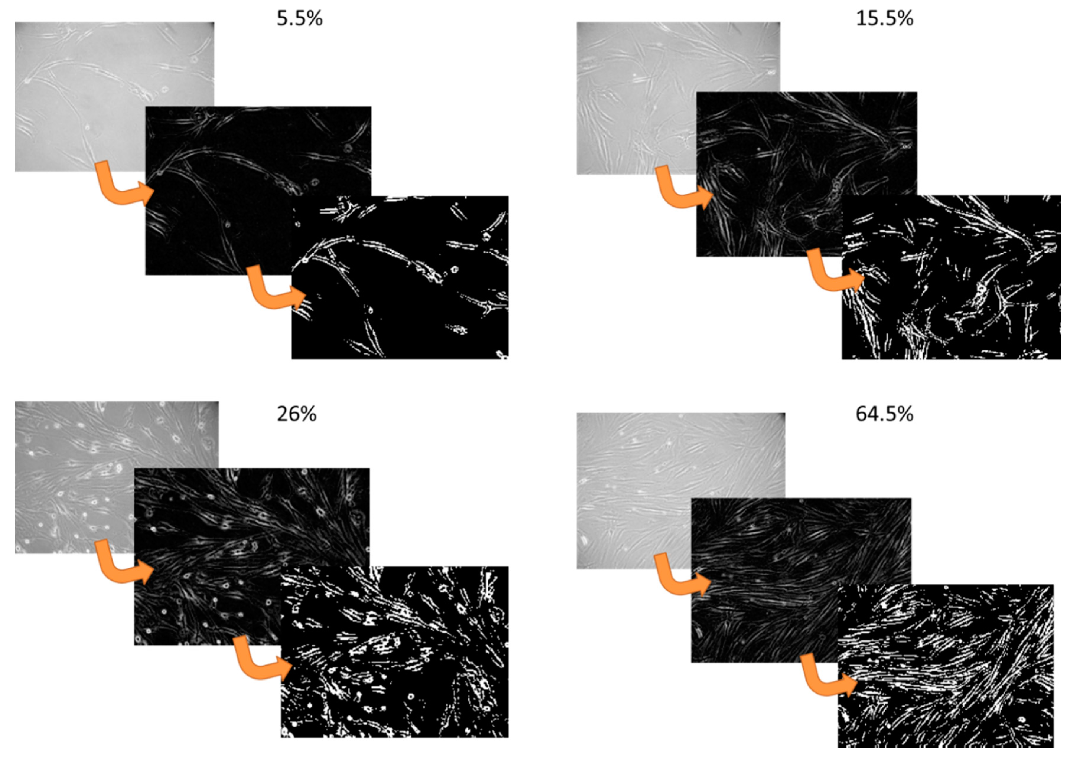
3.1. Acquisition and Processing of Cell Culture Images
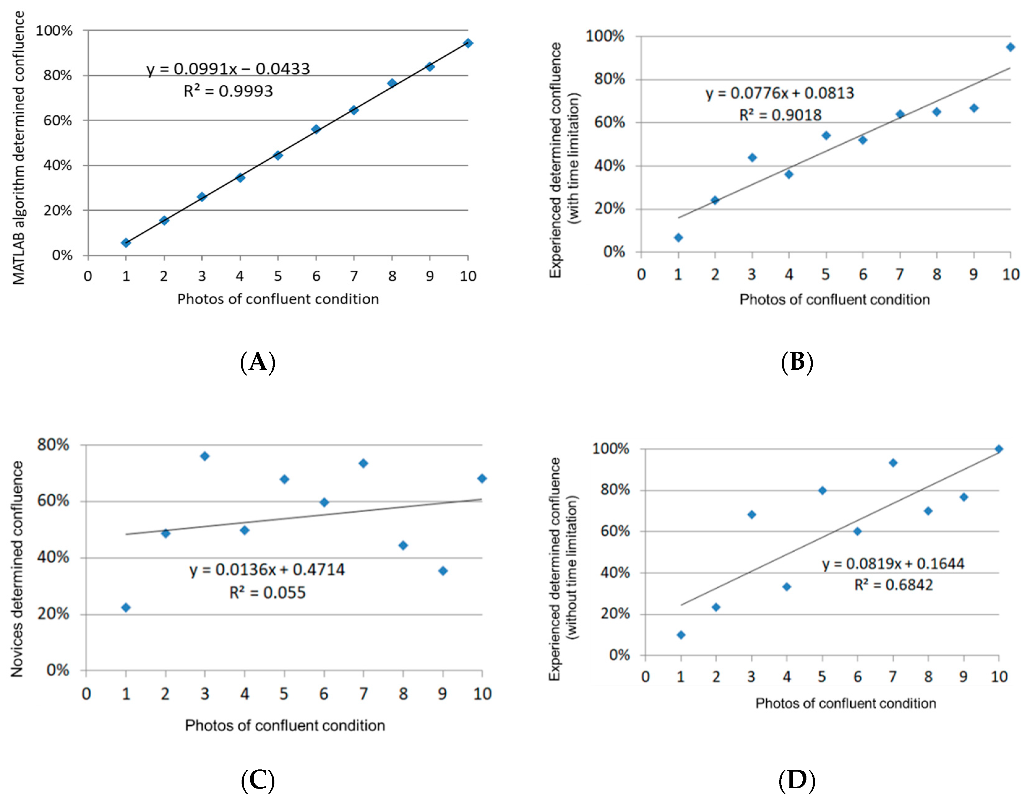
3.2. Determination of Cell Confluence
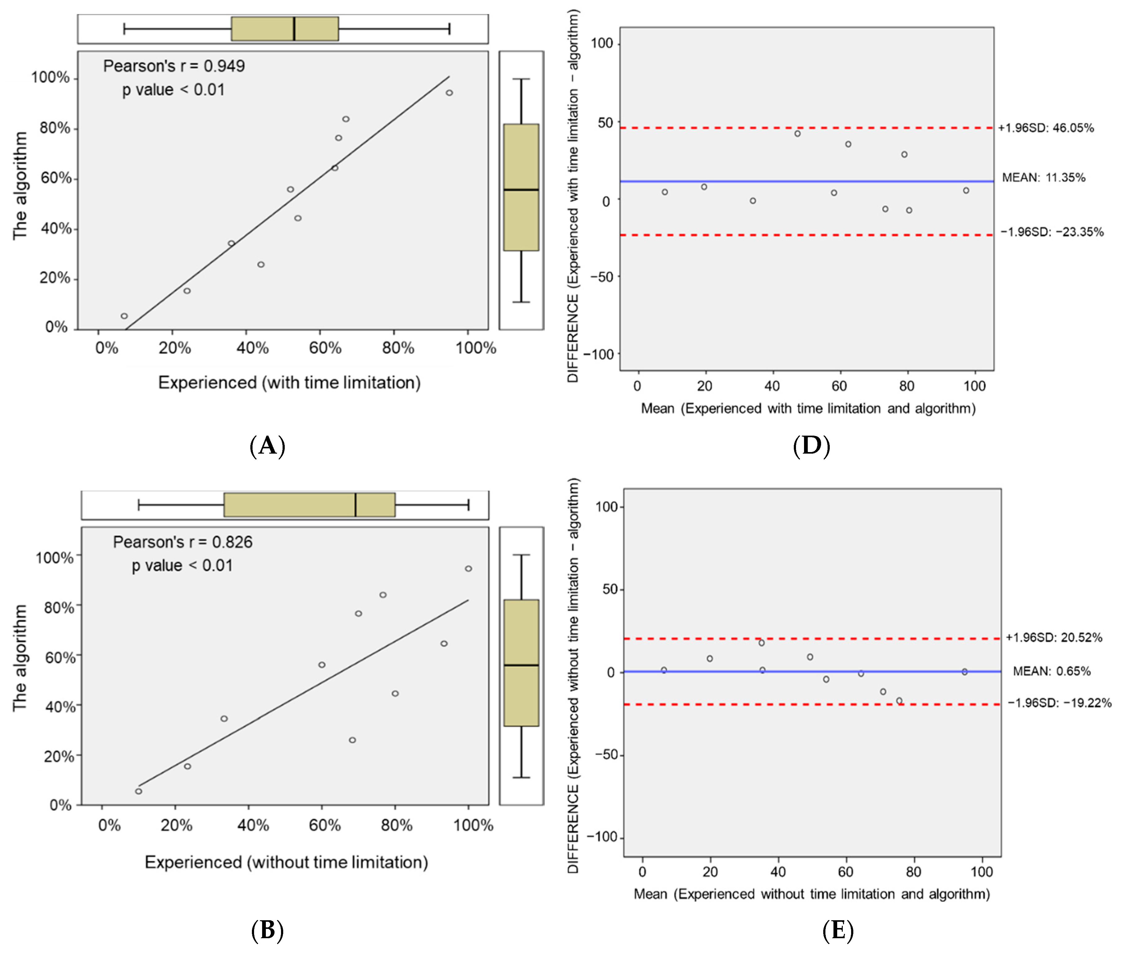
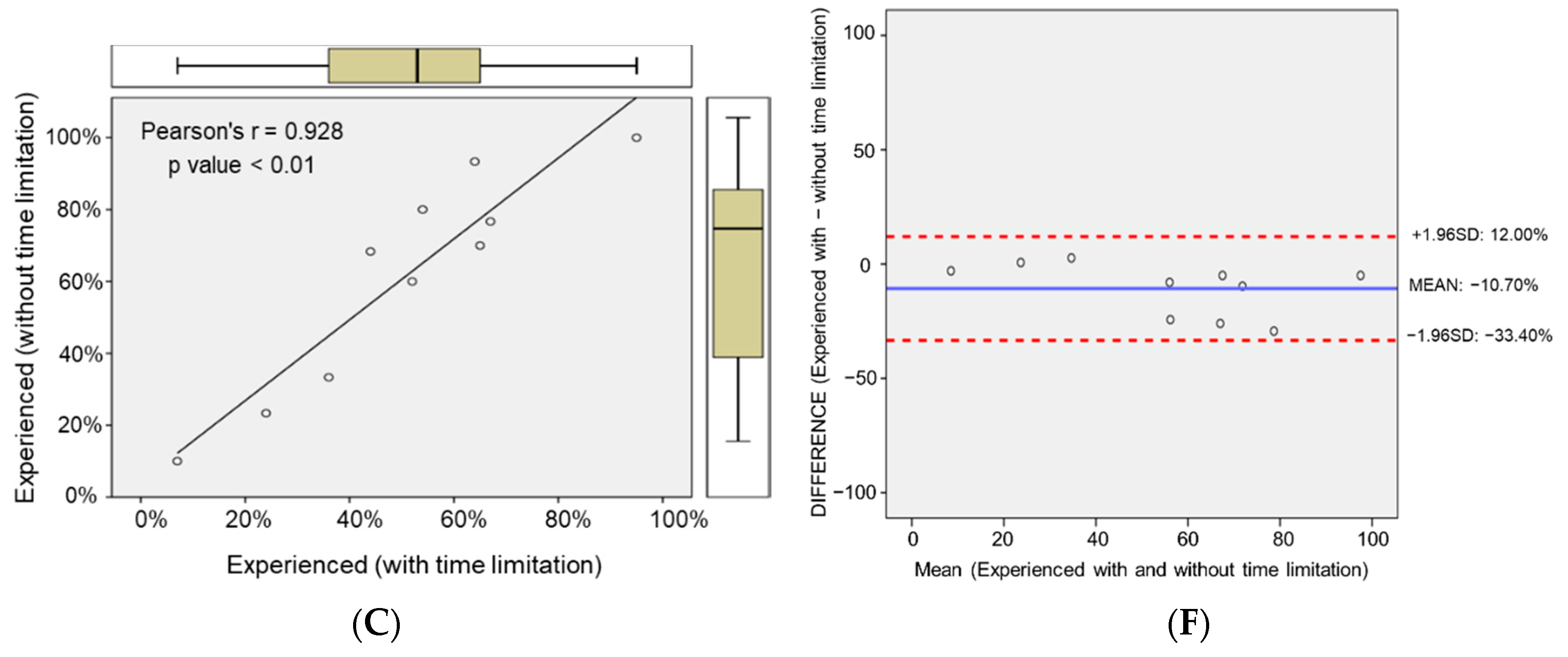
3.3. The Correlation of Cell Confluence Predicted by Novice Students and Experienced Researchers
3.4. The Correlation of Cell Confluence Predicted by Experienced Researchers and the Algorithm
4. Discussion
5. Conclusions
Author Contributions
Funding
Acknowledgments
Conflicts of Interest
References
- Iloki Assanga, S.B.; Gil-Salido, A.A.; Lewis Luján, L.M.; Rosas-Durazo, A.; Acosta-Silva, A.L.; Rivera-Castañeda, E.G.; Rubio-Pino, J.L. Cell growth curves for different cell lines and their relationship with biological activities. Int. J. Biotechnol. Mol. Biol. Res. 2013, 4, 10. [Google Scholar] [CrossRef]
- Savage, N. Computer logic meets cell biology: How cell science is getting an upgrade. Nature 2018, 564, S1–S3. [Google Scholar] [CrossRef] [PubMed]
- Jones, D.T. Setting the standards for machine learning in biology. Nat. Rev. Mol. Cell Biol. 2019, 20, 659–660. [Google Scholar] [CrossRef] [PubMed]
- Browning, L.; Colling, R.; Rakha, E.; Rajpoot, N.; Rittscher, J.; James, J.A.; Salto-Tellez, M.; Snead, D.R.J.; Verrill, C. Digital pathology and artificial intelligence will be key to supporting clinical and academic cellular pathology through COVID-19 and future crises: The PathLAKE consortium perspective. J. Clin. Pathol. 2020. [Google Scholar] [CrossRef]
- Ibrahim, A.; Gamble, P.; Jaroensri, R.; Abdelsamea, M.M.; Mermel, C.H.; Chen, P.C.; Rakha, E.A. Artificial intelligence in digital breast pathology: Techniques and applications. Breast 2020, 49, 267–273. [Google Scholar] [CrossRef] [Green Version]
- Bera, K.; Schalper, K.A.; Rimm, D.L.; Velcheti, V.; Madabhushi, A. Artificial intelligence in digital pathology—New tools for diagnosis and precision oncology. Nat. Rev. Clin. Oncol. 2019, 16, 703–715. [Google Scholar] [CrossRef]
- Niazi, M.K.K.; Parwani, A.V.; Gurcan, M.N. Digital pathology and artificial intelligence. Lancet Oncol. 2019, 20, e253–e261. [Google Scholar] [CrossRef]
- Chan, S.; Bailey, J.; Ros, P.R. Artificial Intelligence in Radiology: Summary of the AUR Academic Radiology and Industry Leaders Roundtable. Acad. Radiol. 2020, 27, 117–120. [Google Scholar] [CrossRef] [Green Version]
- Jha, S.; Cook, T. Artificial Intelligence in Radiology—The State of the Future. Acad. Radiol. 2020, 27, 1–2. [Google Scholar] [CrossRef] [Green Version]
- Weisberg, E.M.; Chu, L.C.; Park, S.; Yuille, A.L.; Kinzler, K.W.; Vogelstein, B.; Fishman, E.K. Deep lessons learned: Radiology, oncology, pathology, and computer science experts unite around artificial intelligence to strive for earlier pancreatic cancer diagnosis. Diagn. Interv. Imaging 2020, 101, 111–115. [Google Scholar] [CrossRef]
- Weikert, T.; Cyriac, J.; Yang, S.; Nesic, I.; Parmar, V.; Stieltjes, B. A Practical Guide to Artificial Intelligence-Based Image Analysis in Radiology. Investig. Radiol. 2020, 55, 1–7. [Google Scholar] [CrossRef] [PubMed]
- Colling, R.; Pitman, H.; Oien, K.; Rajpoot, N.; Macklin, P.; CM-Path AI in Histopathology Working Group; Snead, D.; Sackville, T.; Verrill, C. Artificial intelligence in digital pathology: A roadmap to routine use in clinical practice. J. Pathol. 2019, 249, 143–150. [Google Scholar] [CrossRef] [PubMed]
- Bray, M.A.; Carpenter, A.E. Quality Control for High-Throughput Imaging Experiments Using Machine Learning in Cellprofiler. Methods Mol. Biol. 2018, 1683, 89–112. [Google Scholar] [CrossRef] [PubMed]
- Cheng, D.C.; Wu, J.F.; Kao, Y.H.; Su, C.H.; Liu, S.H. Accurate Measurement of Cross-Sectional Area of Femoral Artery on MRI Sequences of Transcontinental Ultramarathon Runners Using Optimal Parameters Selection. J. Med. Syst. 2016, 40, 260. [Google Scholar] [CrossRef]
- Cheng, D.C.; Wu, J.F.; Kao, Y.H.; Su, C.H.; Liu, S.H. Elliptic Shape Prior Dynamic Programming for Accurate Vessel Segmentation in MRI Sequences with Automated Optimal Parameter Selection. J. Med. Biol. Eng. 2016, 2, 1–9. [Google Scholar] [CrossRef]
- Cheng, D.C.; Chen, L.W.; Shen, Y.W.; Fuh, L.J. Computer-assisted system on mandibular canal detection. Biomed. Tech. 2017, 62, 575–580. [Google Scholar] [CrossRef]
- Tsai, Y.H.; Chen, H.C.; Tung, H.; Wu, Y.Y.; Chen, H.M.; Pan, K.J.; Cheng, D.C.; Chen, J.H.; Chen, C.C.; Chai, J.W.; et al. Noninvasive assessment of intracranial elastance and pressure in spontaneous intracranial hypotension by MRI. J. Magn. Reson. Imaging 2018, 48, 1255–1263. [Google Scholar] [CrossRef]
- Cheng, D.C.; Chi, J.H.; Yang, S.N.; Liu, S.H. Organ Contouring for Lung Cancer Patients with a Seed Generation Scheme and Random Walks. Sensors 2020, 20, 4823. [Google Scholar] [CrossRef]
- Cadena-Herrera, D.; Esparza-De Lara, J.E.; Ramirez-Ibanez, N.D.; Lopez-Morales, C.A.; Perez, N.O.; Flores-Ortiz, L.F.; Medina-Rivero, E. Validation of three viable-cell counting methods: Manual, semi-automated, and automated. Biotechnol. Rep. 2015, 7, 9–16. [Google Scholar] [CrossRef] [Green Version]
- Vembadi, A.; Menachery, A.; Qasaimeh, M.A. Cell Cytometry: Review and Perspective on Biotechnological Advances. Front. Bioeng. Biotechnol. 2019, 7, 147. [Google Scholar] [CrossRef]
- Meijering, E. Cell Segmentation: 50 Years Down the Road. IEEE Signal Process. Mag. 2012, 29, 140–145. [Google Scholar] [CrossRef]
- Vicar, T.; Balvan, J.; Jaros, J.; Jug, F.; Kolar, R.; Masarik, M.; Gumulec, J. Cell segmentation methods for label-free contrast microscopy: Review and comprehensive comparison. BMC Bioinform. 2019, 20, 360. [Google Scholar] [CrossRef] [PubMed]
- Hilsenbeck, O.; Schwarzfischer, M.; Skylaki, S.; Schauberger, B.; Hoppe, P.S.; Loeffler, D.; Kokkaliaris, K.D.; Hastreiter, S.; Skylaki, E.; Filipczyk, A.; et al. Software tools for single-cell tracking and quantification of cellular and molecular properties. Nat. Biotechnol. 2016, 34, 703–706. [Google Scholar] [CrossRef]
- Available online: https://paperswithcode.com/task/cell-segmentation/codeless (accessed on 20 October 2020).
- Available online: https://www.mathworks.com/matlabcentral/fileexchange/82370-confluence-viewer (accessed on 20 October 2020).
- Available online: https://au.mathworks.com/matlabcentral/fileexchange/82375-confluence-viewer-cell-images-for-constructing-a-model (accessed on 20 October 2020).
- Wright Muelas, M.; Ortega, F.; Breitling, R.; Bendtsen, C.; Westerhoff, H.V. Rational cell culture optimization enhances experimental reproducibility in cancer cells. Sci. Rep. 2018, 8, 3029. [Google Scholar] [CrossRef] [PubMed] [Green Version]
- Busschots, S.; O’Toole, S.; O’Leary, J.J.; Stordal, B. Non-invasive and non-destructive measurements of confluence in cultured adherent cell lines. MethodsX 2015, 2, 8–13. [Google Scholar] [CrossRef] [PubMed]


Publisher’s Note: MDPI stays neutral with regard to jurisdictional claims in published maps and institutional affiliations. |
© 2020 by the authors. Licensee MDPI, Basel, Switzerland. This article is an open access article distributed under the terms and conditions of the Creative Commons Attribution (CC BY) license (http://creativecommons.org/licenses/by/4.0/).
Share and Cite
Chiu, C.-H.; Leu, J.-D.; Lin, T.-T.; Su, P.-H.; Li, W.-C.; Lee, Y.-J.; Cheng, D.-C. Systematic Quantification of Cell Confluence in Human Normal Oral Fibroblasts. Appl. Sci. 2020, 10, 9146. https://doi.org/10.3390/app10249146
Chiu C-H, Leu J-D, Lin T-T, Su P-H, Li W-C, Lee Y-J, Cheng D-C. Systematic Quantification of Cell Confluence in Human Normal Oral Fibroblasts. Applied Sciences. 2020; 10(24):9146. https://doi.org/10.3390/app10249146
Chicago/Turabian StyleChiu, Ching-Hsiang, Jyh-Der Leu, Tzu-Ting Lin, Pin-Hua Su, Wan-Chun Li, Yi-Jang Lee, and Da-Chuan Cheng. 2020. "Systematic Quantification of Cell Confluence in Human Normal Oral Fibroblasts" Applied Sciences 10, no. 24: 9146. https://doi.org/10.3390/app10249146