Evolutionary Design Optimization of an Alkaline Water Electrolysis Cell for Hydrogen Production

 ,
,  , ,
, ,  , ,
, ,  , and
, and
Abstract
:Featured Application
Abstract
1. Introduction
2. Physics and Economy of the Alkaline Water Electrolysis Cell
2.1. Theory
2.2. Physics of the Void Fraction
2.2.1. Mathematical and Numerical Tools
- Finite Volume Model (CFD)
- The flow is Newtonian, viscous and incompressible;
- the flow is considered isothermal;
- ions distributions are neglected;
- the flow is considered laminar;
- bubble diameter is constant for a given operating condition; and
- The current density is taken as constant.
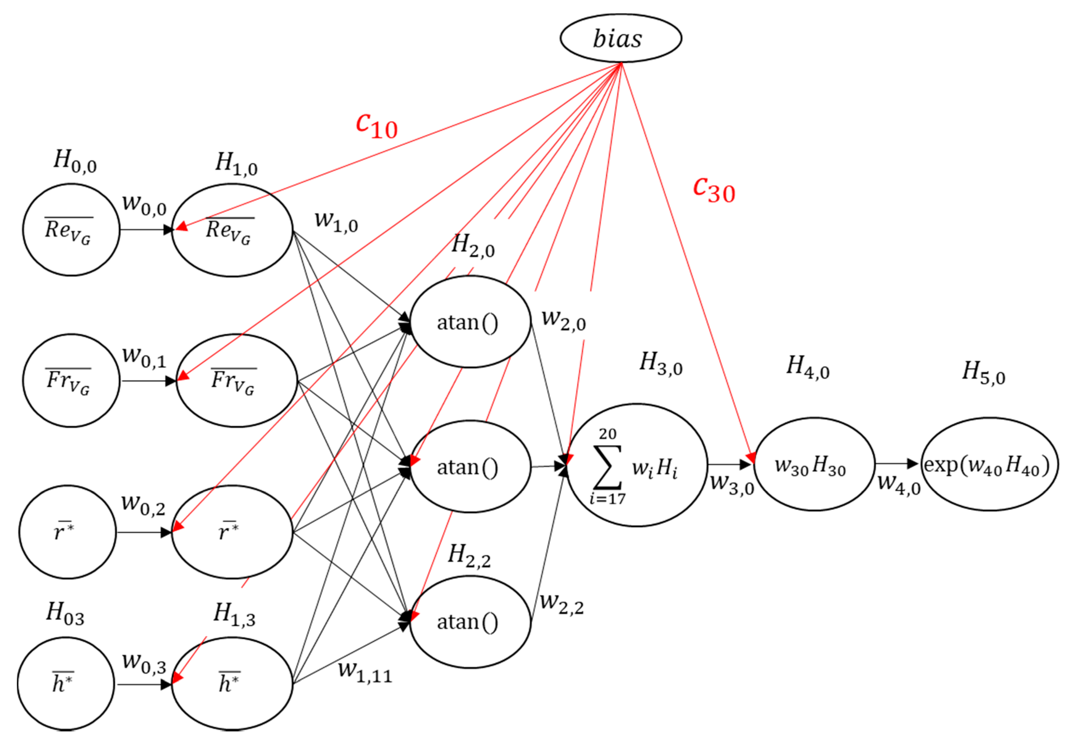
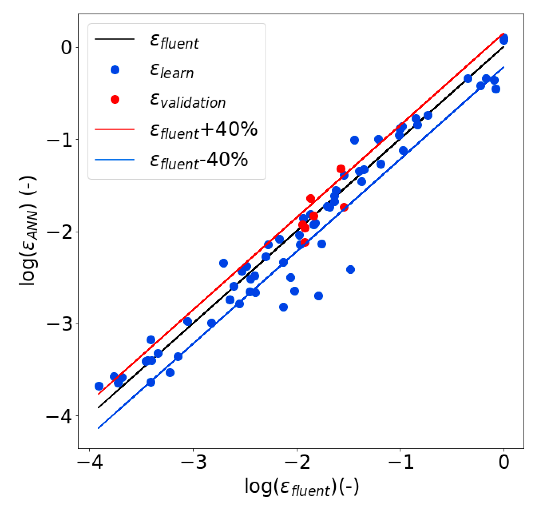
- Artificial Neural Network (ANN)
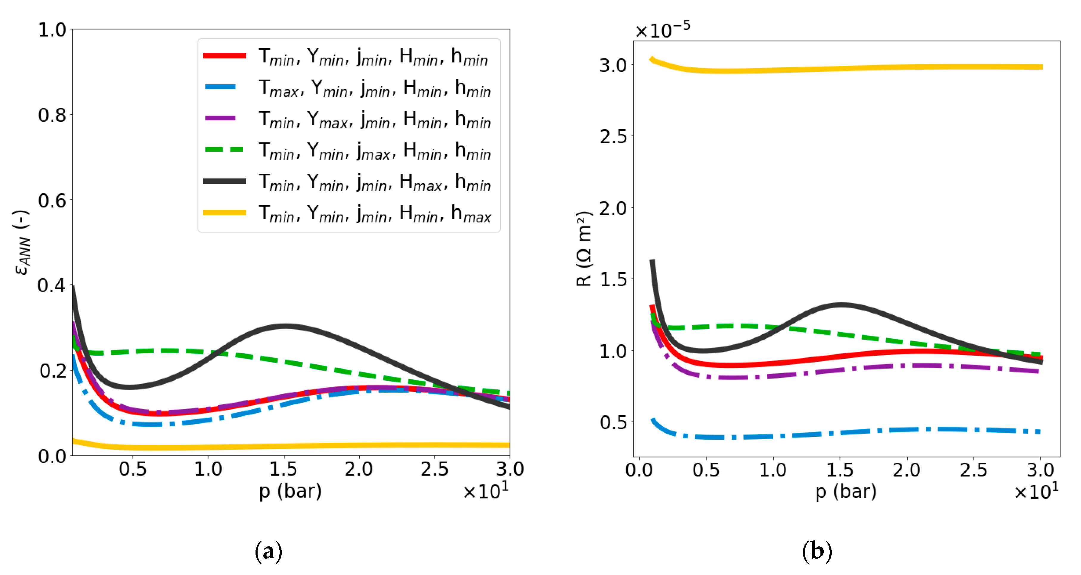
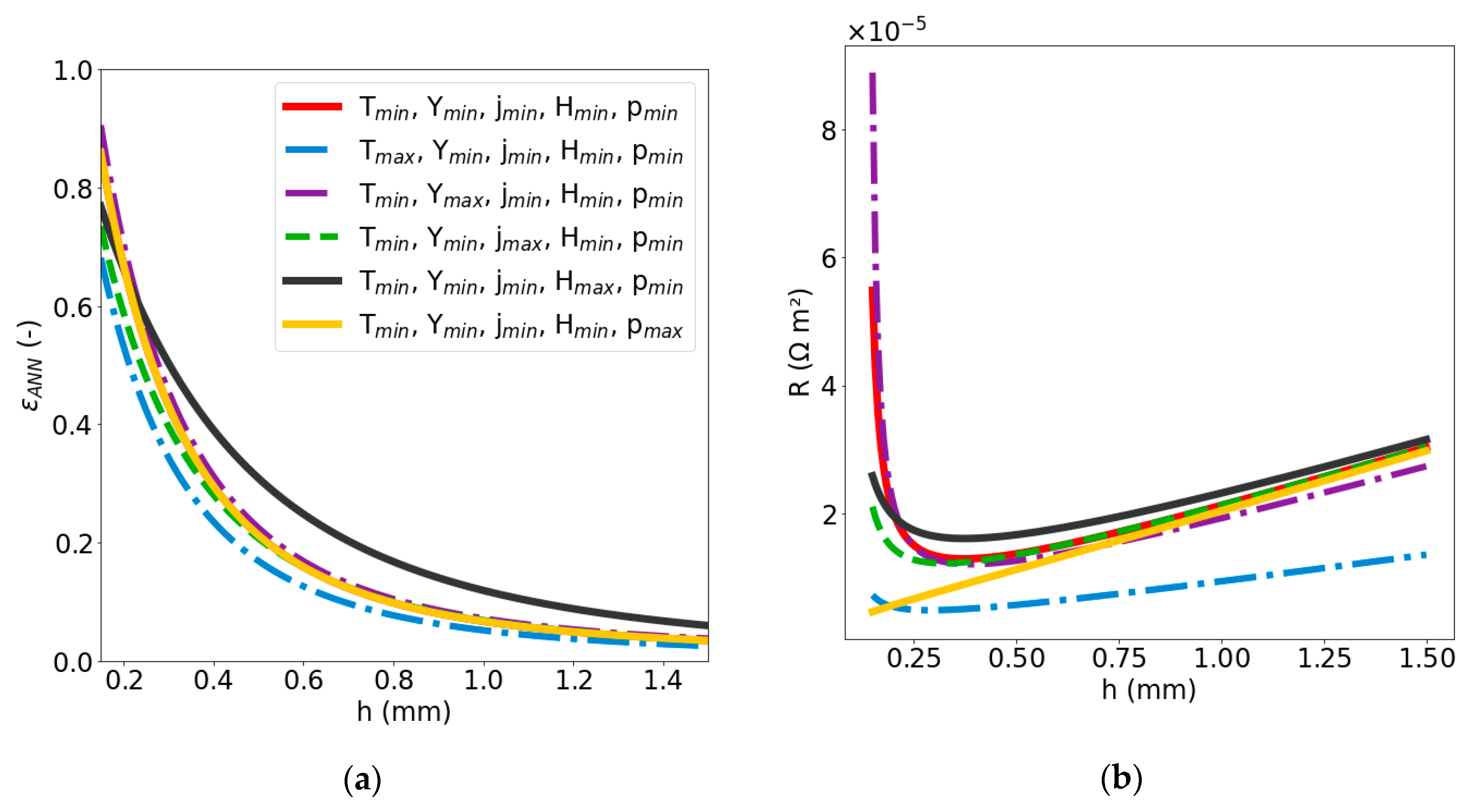
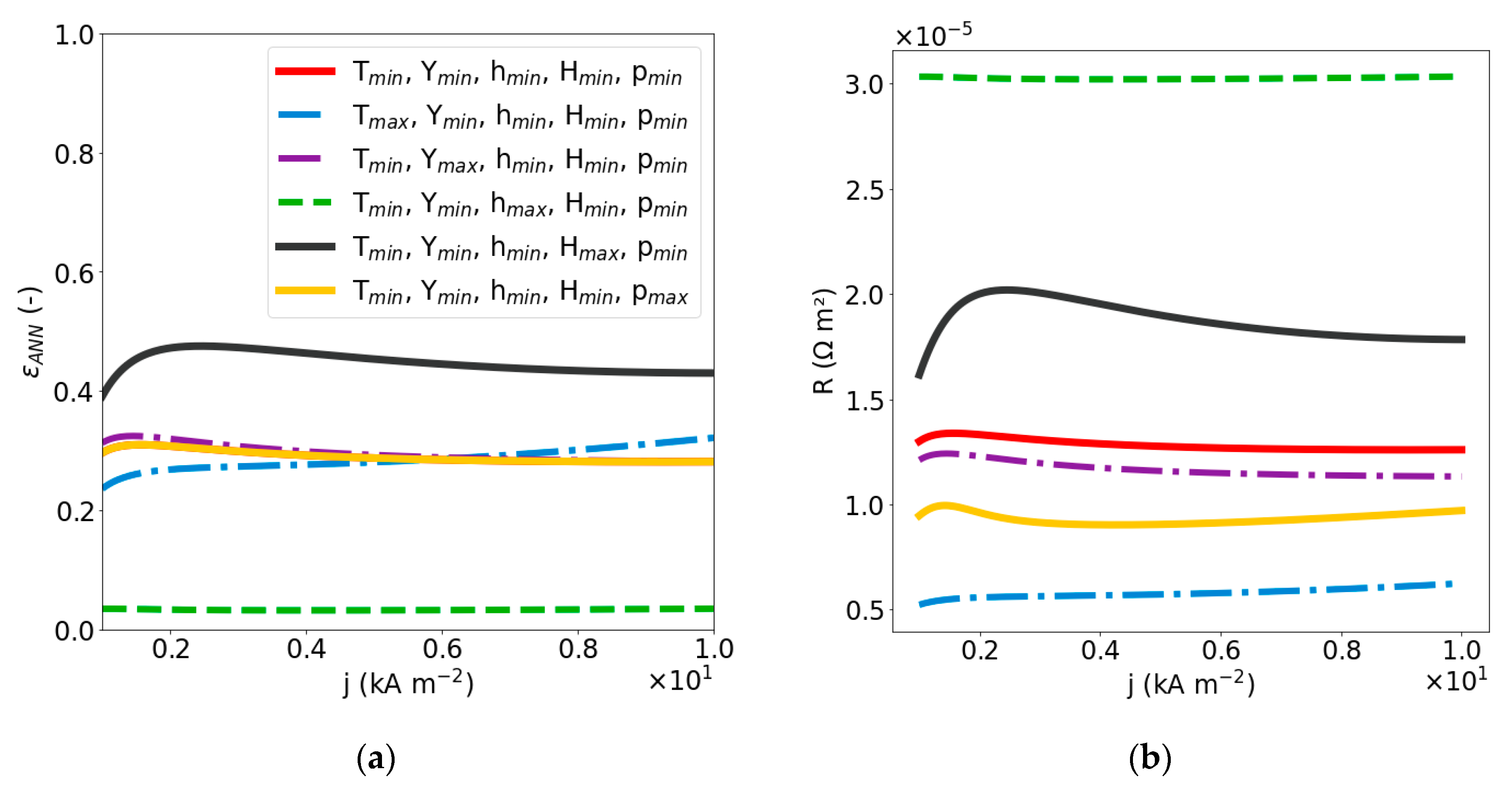
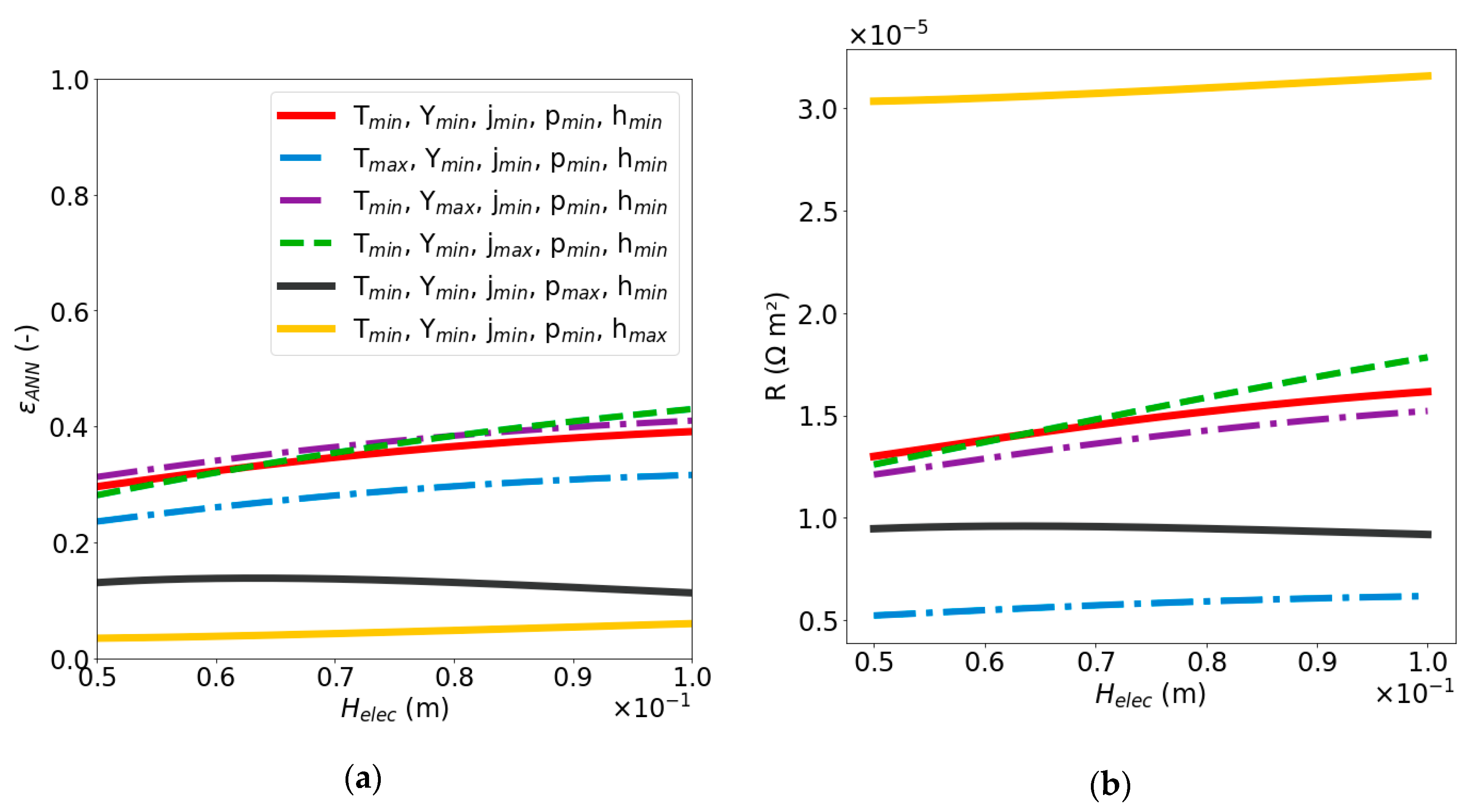
2.2.2. Sensitivity Analysis of Void Fraction and Ohmic Resistance
2.3. Economy
3. Set up of the Genetic Algorithm
3.1. Optimization Problem
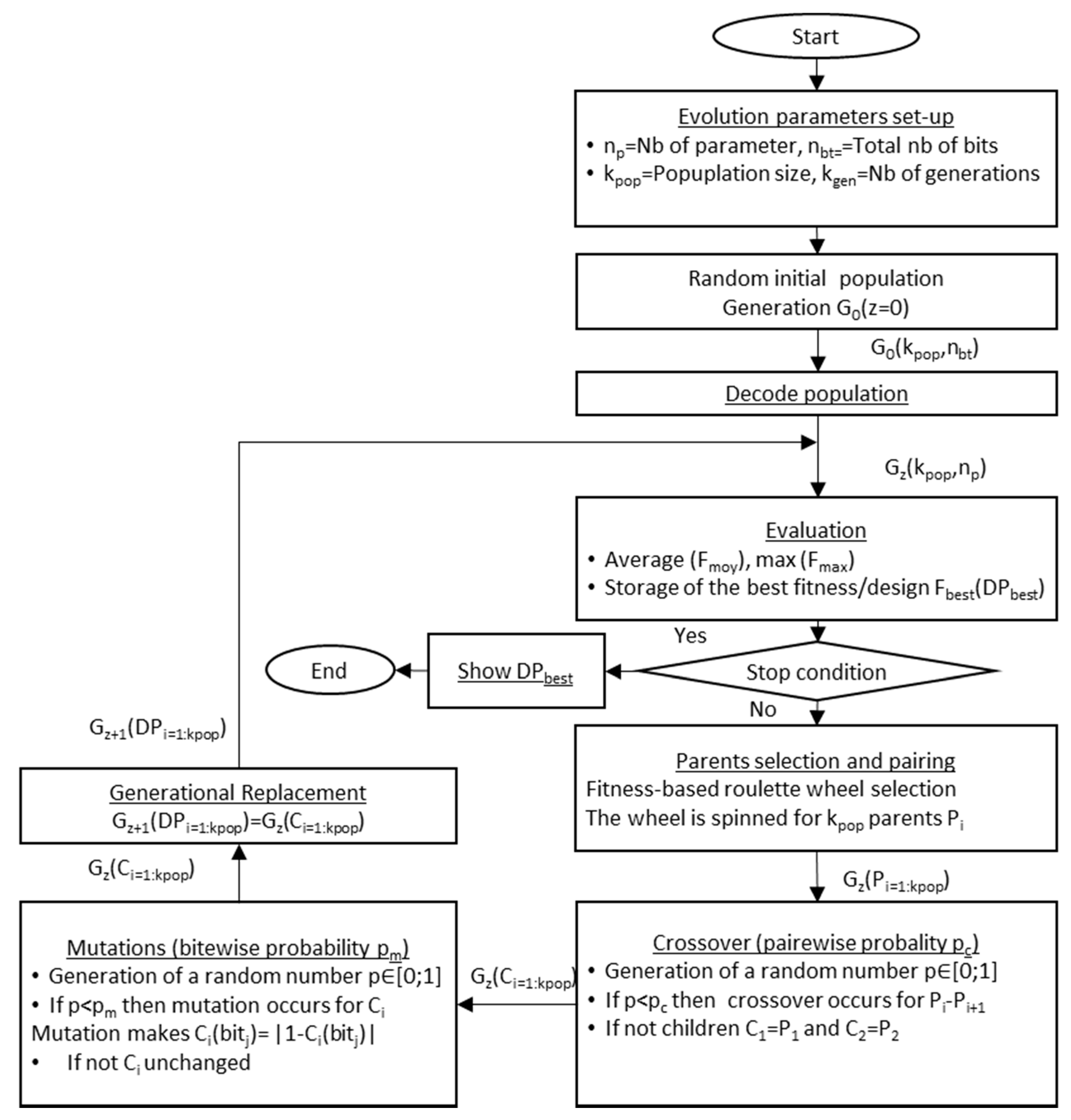
3.2. Genetic Optimization Algorithm (GA)
3.3. Coding
3.4. Evaluation
3.5. Operators
3.5.1. Initial Random Population
3.5.2. Roulette Wheel Selection
3.5.3. Single Point Crossing-Over
3.5.4. Bitwise Mutation
3.5.5. Replacement Generator (Generational)
3.5.6. Presentation of the Evolution Parameter
- the number of generations
- the number of populations per generation
- probability of mutation
- probability of crossing-over is definitively set to 50%
3.6. Validation of the Algorithm
- = 800 € m−2
- = 17c€ kWh−1
- = = 0.15 V dec−1
- = 3.23 × 10⁻⁵ Ohm m2 [27]
- The simplified model does not take into account the two-phase phenomena, which can greatly influence the hydrogen costs ().
- The evolution parameters used in this first try are not well adapted to the problem (missing convergence phase to achieve evolution).
4. Sensitivity Study of the Results to the Evolution Parameters
- = 800 € m−2
- = 17 c€ kWh−1
- = = 0.15 V dec−1
- = 3.23 × 10⁻⁵ Ohm m2
- = 25 × 10−6 m
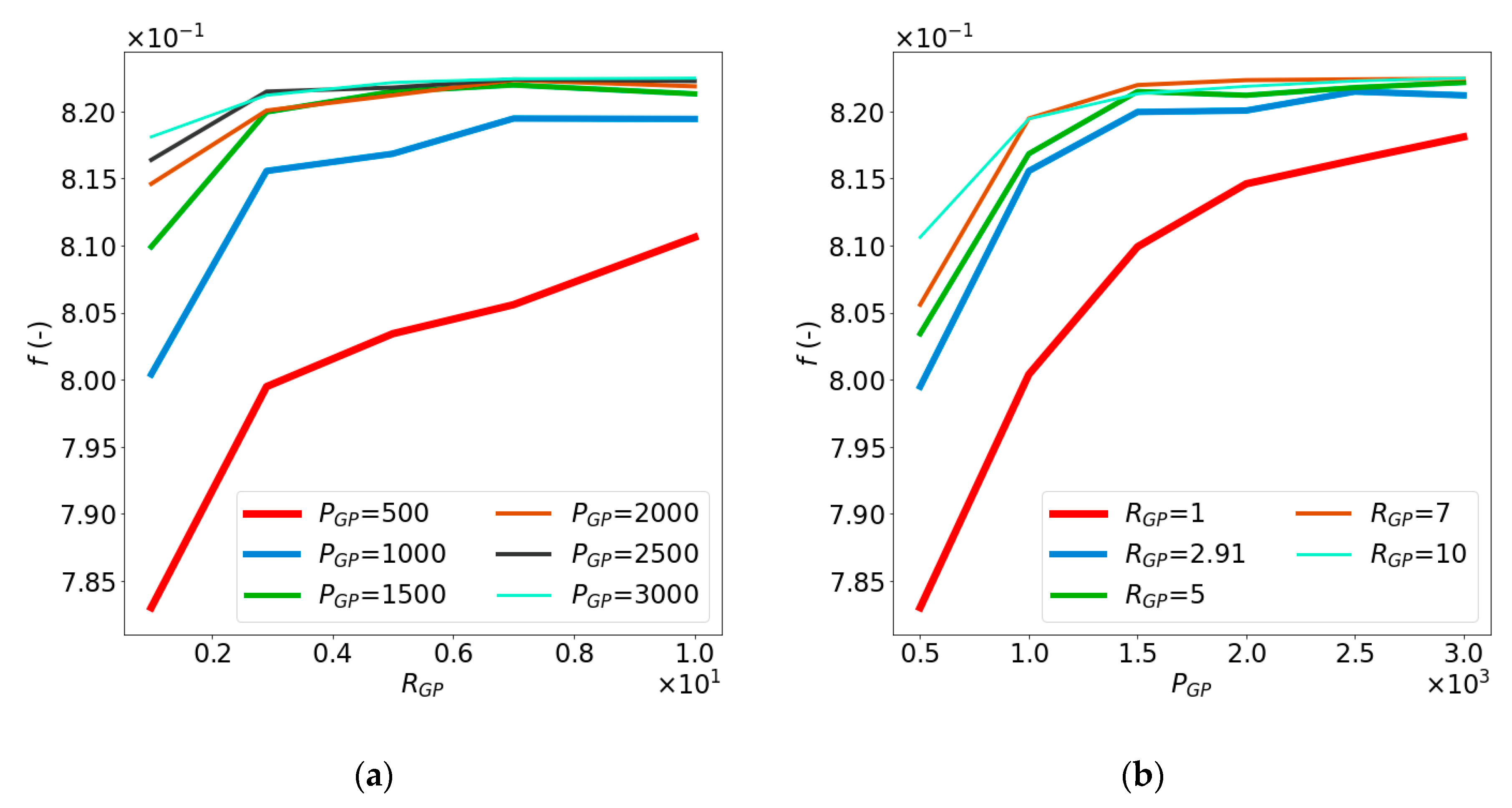
4.1. Impact of and
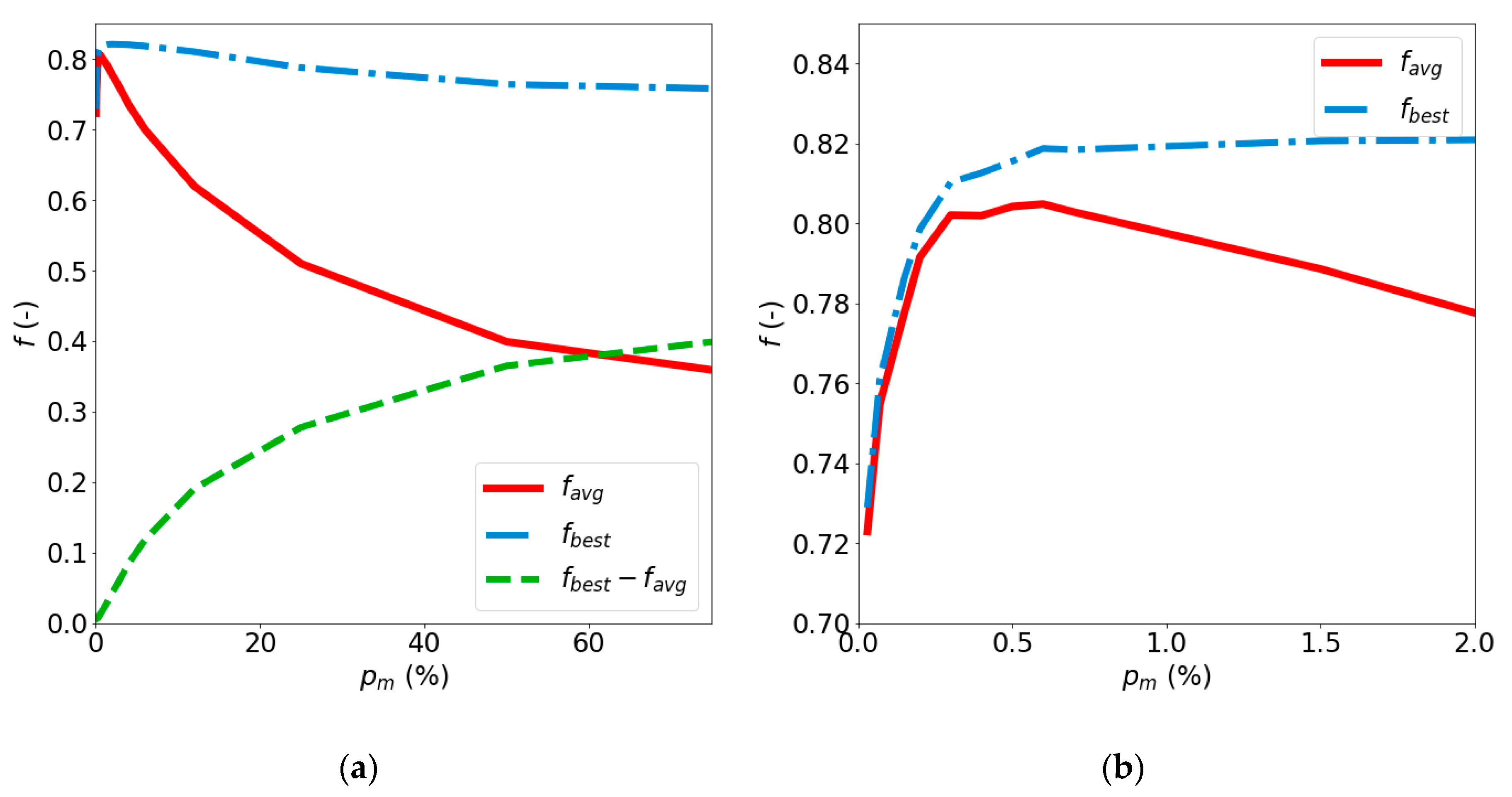
4.2. Impact of pm
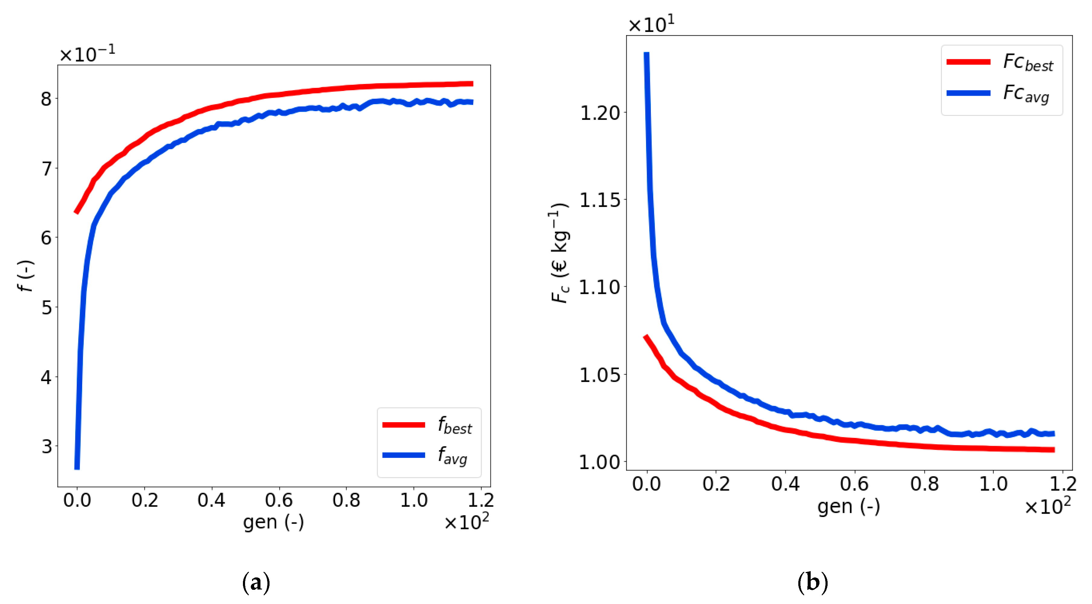
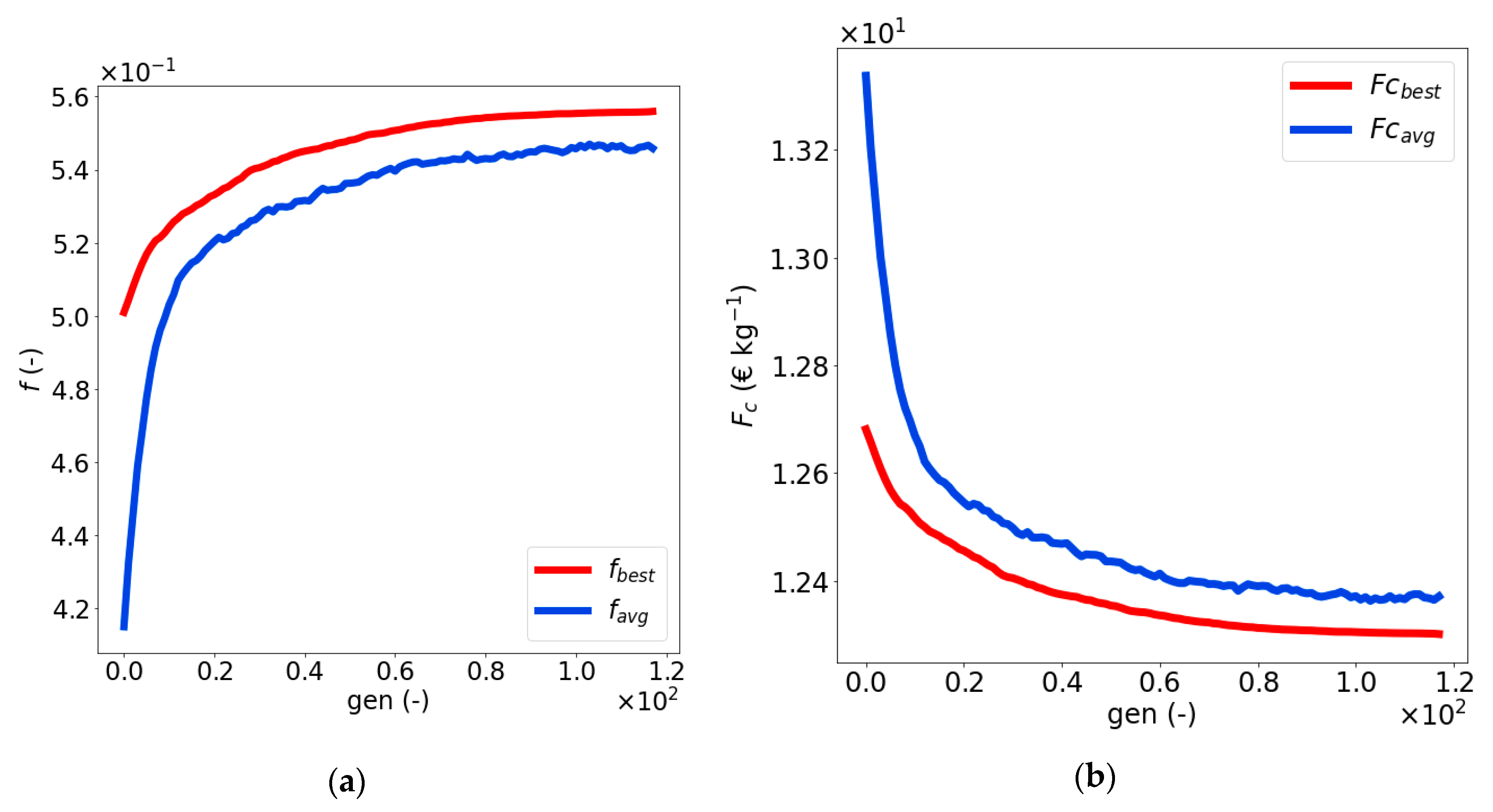
4.3. Optimization of the Naïve Solution
5. Conclusions
Author Contributions
Funding
Acknowledgments
Conflicts of Interest
Appendix A
Appendix B

| N° | |||||
|---|---|---|---|---|---|
| 1 | −0.375 | 1 | 0.625 | −0.25 | 2.07 × 10⁻⁴ |
| 2 | −0.875 | −0.5 | 0.75 | 0.125 | 3.52 × 10⁻⁴ |
| 3 | −0.75 | −0.125 | −0.875 | −0.5 | 1.95 × 10⁻³ |
| 4 | −0.625 | 0.25 | −0.375 | 1 | 3.868 × 10⁻⁴ |
| 5 | 0.5 | 0.875 | −0.125 | −0.75 | 3.972 × 10⁻⁴ |
| 6 | 1 | −0.375 | −0.25 | 0.625 | 4.543 × 10⁻⁴ |
| 7 | 0.25 | −0.625 | 1 | −0.375 | 3.884 × 10⁻⁴ |
| 8 | 0.125 | 0.75 | 0.5 | 0.875 | 1.737 × 10⁻⁴ |
| 9 | 0 | 0 | 0 | 0 | 3.624 × 10⁻⁴ |
| 10 | 0.375 | −1 | −0.625 | 0.25 | 1.477 × 10⁻¹ |
| 11 | 0.875 | 0.5 | −0.75 | −0.125 | 8.782 × 10⁻⁴ |
| 12 | 0.75 | 0.125 | 0.875 | 0.5 | 1.897 × 10⁻⁴ |
| 13 | 0.625 | −0.25 | 0.375 | −1 | 5.931 × 10⁻⁴ |
| 14 | −0.5 | −0.875 | 0.125 | 0.75 | 7.161 × 10⁻⁴ |
| 15 | −1 | 0.375 | 0.25 | −0.625 | 5.067 × 10⁻³ |
| 16 | −0.25 | 0.625 | −1 | 0.375 | 3.289 × 10⁻³ |
| 17 | −0.125 | −0.75 | −0.5 | −0.875 | 1.515 × 10⁻³ |
| 18 | 1 | −1 | −1 | 1 | 1 |
| 19 | 1 | 1 | 1 | 1 | 1.219 × 10⁻⁴ |
| 20 | −1 | −1 | 1 | 1 | 1.856 × 10⁻¹ |
| 21 | 1 | −1 | 1 | −1 | 2.096 × 10⁻² |
| 22 | −1 | 1 | −1 | 1 | 1.063 × 10⁻¹ |
| 23 | −1 | 1 | 1 | −1 | 2.935 × 10⁻³ |
| 24 | 1 | 1 | −1 | −1 | 3.986 × 10⁻³ |
| 25 | −1 | −1 | −1 | −1 | 1 |
| 26 | −0.9325 | −0.98 | −0.95 | −1 | 4.058 × 10⁻² |
| 27 | −0.9325 | −1 | −0.875 | 1 | 6.778 × 10⁻¹ |
| 28 | −0.99 | −0.99 | −0.95 | 1 | 9.828 × 10⁻² |
| 29 | −0.875 | −0.99 | −0.875 | −1 | 2.301 × 10⁻² |
| 30 | −0.99 | −0.98 | −0.875 | 0 | 4.274 × 10⁻² |
| 31 | −0.875 | −1 | −0.95 | 0 | 8.424 × 10⁻¹ |
| 32 | −0.946 | −0.990 | −0.728 | −0.427 | 1.460 × 10⁻² |
| 33 | −0.983 | −0.997 | −0.704 | −0.200 | 4.440 × 10⁻² |
| 34 | −0.973 | −0.996 | −1.023 | −0.578 | 4.539 × 10⁻¹ |
| 35 | −0.964 | −0.994 | −0.925 | 0.328 | 6.174 × 10⁻² |
| 36 | −0.881 | −0.991 | −0.876 | −0.729 | 2.390 × 10⁻² |
| 37 | −0.844 | −0.997 | −0.900 | 0.101 | 3.623 × 10⁻² |
| 38 | −0.900 | −0.998 | −0.655 | −0.503 | 1.993 × 10⁻² |
| 39 | −0.909 | −0.992 | −0.753 | 0.252 | 1.350 × 10⁻² |
| 40 | −0.918 | −0.995 | −0.851 | −0.276 | 2.892 × 10⁻² |
| 41 | −0.890 | −0.999 | −0.974 | −0.125 | 8.122 × 10⁻¹ |
| 42 | −0.853 | −0.993 | −0.999 | −0.352 | 1.044 × 10⁻¹ |
| 43 | −0.863 | −0.994 | −0.679 | 0.026 | 1.155 × 10⁻² |
| 44 | −0.872 | −0.996 | −0.778 | −0.881 | 2.310 × 10⁻² |
| 45 | −0.955 | −0.999 | −0.827 | 0.177 | 9.900 × 10⁻² |
| 46 | −0.992 | −0.993 | −0.802 | −0.654 | 6.528 × 10⁻² |
| 47 | −0.937 | −0.992 | −1.048 | −0.050 | 6.000 × 10⁻¹ |
| 48 | −0.927 | −0.998 | −0.95 | −0.805 | 1.431 × 10⁻¹ |
| 49 | −0.8 | −0.87 | −0.85 | −0.875 | 5.296 × 10⁻³ |
| 50 | −0.8 | −0.97 | −0.55 | −0.125 | 3.516 × 10⁻³ |
| 51 | −0.9 | −0.92 | −0.85 | −0.125 | 6.844 × 10⁻³ |
| 52 | −0.7 | −0.92 | −0.55 | −0.875 | 2.807 × 10⁻³ |
| 53 | −0.9 | −0.97 | −0.7 | −0.875 | 7.510 × 10⁻³ |
| 54 | −0.7 | −0.87 | −0.7 | −0.125 | 2.482 × 10⁻³ |
| 55 | −0.9 | −0.87 | −0.55 | −0.5 | 2.279 × 10⁻³ |
| 56 | −0.7 | −0.97 | −0.85 | −0.5 | 1.068 × 10⁻² |
| 57 | −0.8 | −0.92 | −0.7 | −0.5 | 3.584 × 10⁻³ |
| 58 | −0.8 | −0.87 | −0.85 | −1 | 1.740 × 10⁻² |
| 59 | −0.8 | −0.97 | −0.55 | −0.9 | 9.525 × 10⁻³ |
| 60 | −0.7 | −0.92 | −0.85 | −0.9 | 1.082 × 10⁻² |
| 61 | −0.9 | −0.92 | −0.55 | −1 | 1.636 × 10⁻² |
| 62 | −0.7 | −0.97 | −0.7 | −1 | 3296 × 10−2 |
| 63 | −0.9 | −0.87 | −0.7 | −0.9 | 3899 × 10−3 |
| 64 | −0.7 | −0.87 | −0.55 | −0.95 | 7417 × 10−3 |
| 65 | −0.9 | −0.97 | −0.85 | −0.95 | 1508 × 10−2 |
References
- Le Bideau, D.; Mandin, P.; Benbouzid, M.; Kim, M.; Sellier, M.; Ganci, F.; Inguanta, R. Eulerian Two-Fluid Model of Alkaline Water Electrolysis for Hydrogen Production. Energies 2020, 13, 3394. [Google Scholar] [CrossRef]
- Schillings, J.; Doche, O.; Deseure, J. Modeling of electrochemically generated bubbly flow under buoyancy-driven and forced convection. Int. J. Heat Mass Transf. 2015, 85, 292–299. [Google Scholar] [CrossRef]
- Mat, M. A two-phase flow model for hydrogen evolution in an electrochemical cell. Int. J. Hydrog. Energy 2004, 29, 1015–1023. [Google Scholar] [CrossRef]
- Dahlkild, A. Modelling the two-phase flow and current distribution along a vertical gas-evolving electrode. J. Fluid Mech. 2001, 428, 249–272. [Google Scholar] [CrossRef]
- Wedin, R.; Dahlkild, A. On the Transport of Small Bubbles under Developing Channel Flow in a Buoyant Gas-Evolving Electrochemical Cell. Ind. Eng. Chem. Res. 2001, 40, 5228–5233. [Google Scholar] [CrossRef]
- Ulleberg, O. Modeling of advanced alkaline electrolyzers: A system simulation approach. Int. J. Hydrog. Energy 2003, 28, 21–33. [Google Scholar] [CrossRef]
- Villagra, A.; Millet, P. An analysis of PEM water electrolysis cells operating at elevated current densities. Int. J. Hydrog. Energy 2019, 44, 9708–9717. [Google Scholar] [CrossRef]
- Bensmann, B.; Hanke-Rauschenbach, R.; Müller-Syring, G.; Henel, M.; Sundmacher, K. Optimal configuration and pressure levels of electrolyzer plants in context of power-to-gas applications. Appl. Energy 2016, 167, 107–124. [Google Scholar] [CrossRef]
- Chocron, O. Evolutionary design of modular robotic arms. Robotica 2008, 26, 323–330. [Google Scholar] [CrossRef]
- Hammoudi, M.; Henao, C.; Agbossou, K.; Dubé, Y.; Doumbia, M. New multi-physics approach for modelling and design of alkaline electrolyzers. Int. J. Hydrog. Energy 2012, 37, 13895–13913. [Google Scholar] [CrossRef]
- Mandin, P.; Derhoumi, Z.; Roustan, H.; Rolf, W. Bubble Over-Potential during Two-Phase Alkaline Water Electrolysis. Electrochim. Acta 2014, 128, 248–258. [Google Scholar] [CrossRef]
- Hine, F.; Murakami, K. Bubble Effects on the Solution IR Drop in a Vertical Electrolyzer under Free and Forced Convection. J. Electrochem. Soc. 1980, 127, 292–297. [Google Scholar] [CrossRef]
- Vogt, H. The Quantities Affecting the Bubble Coverage of Gas-Evolving Electrodes. Electrochim. Acta 2017, 235, 495–499. [Google Scholar] [CrossRef]
- Jannsen, L.J.J.; Sillen, C.W.M.P.; Van Stralen, S.J.D. Bubble behaviour during oxygen and hydrogen evolution at transparent electrodes in KOH solution. Electrochim. Acta 1984, 29, 633–642. [Google Scholar] [CrossRef] [Green Version]
- Gilliam, R.; Graydon, J.; Kirk, D.; Thorpe, S. A review of specific conductivities of potassium hydroxide solutions for various concentrations and temperatures. Int. J. Hydrog. Energy 2007, 32, 359–364. [Google Scholar] [CrossRef]
- See, D.M.; White, R.E. Temperature and Concentration Dependence of the Specific Conductivity of Concentrated Solutions of Potassium Hydroxide. J. Chem. Eng. Data 1997, 42, 1266–1268. [Google Scholar] [CrossRef]
- Le Bideau, D.; Mandin, P.; Benbouzid, M.; Kim, M.; Sellier, M. Review of necessary thermophysical properties and their sensivities with temperature and electrolyte mass fractions for alkaline water electrolysis multiphysics modelling. Int. J. Hydrog. Energy 2019, 44, 4553–4569. [Google Scholar] [CrossRef]
- Grigoriev, S.; Fateev, V.; Bessarabov, D.; Millet, P. Current status, research trends, and challenges in water electrolysis science and technology. Int. J. Hydrog. Energy 2020, 45, 26036–26058. [Google Scholar] [CrossRef]
- Nagai, N. Existence of optimum space between electrodes on hydrogen production by water electrolysis. Int. J. Hydrog. Energy 2003, 28, 35–41. [Google Scholar] [CrossRef] [Green Version]
- Nagai, N.; Ito, T.; Nishijiri, N. Visualization and Numerical Simulation of Two-Phase Flow between Electrodes on Alkaline Water Electrolysis. J. Flow Vis. Image Process. 2010, 17, 99–112. [Google Scholar] [CrossRef]
- Nagai, N.; Takeuchi, M.; Furuta, T. Effects of Bubbles Between Electrodes on Alkaline Water Electrolysis Efficiency Under Forced Convection of Electrolyte. In Proceedings of the 16th World Hydrogen Energy Conference, Lyon, France, 13–16 June 2006. [Google Scholar]
- Vogt, H.; Balzer, R. The bubble coverage of gas-evolving electrodes in stagnant electrolytes. Electrochim. Acta 2005, 50, 2073–2079. [Google Scholar] [CrossRef]
- Boissonneau, P.; Byrne, P. An experimental investigation of bubble-induced free convection in a small electrochemical cell. J. Appl. Electrochem. 2000, 30, 767–775. [Google Scholar] [CrossRef]
- Yu, H.; Wilamowski, B.M. Levenberg–Marquardt Training. In The Industrial Electronics Handbook; CRC Press: Boca Raton, FL, USA, 2011. [Google Scholar]
- Goldberg, D.E. Genetic Algorithms in Search, Optimization and MachineLearning; Addison-Wesley Professional: Boston, MA, USA, 1989. [Google Scholar]
- Chocron, O. Conception Evolutionnaire de Systèmes Robotiques. Ph.D. Thesis, Université Paris, Paris, France, 2000. [Google Scholar]
- Seetharaman, S.; Davidson, D.J.; Vasudeva, S.; Sozhan, G. Polyvinyl Alcohol Based Membrane as Separator for Alkaline Water Electrolyzer. Separ. Sci. Tech. 2011, 46, 1563–1570. [Google Scholar] [CrossRef]


| Dimensionless Parameter | ||||
|---|---|---|---|---|
| 1 × 10⁻² | 300 | 150.005 | 149.995 | |
| 5.85 × 10⁴ | 5.30 × 10¹⁰ | 2.65 × 10¹⁰ | 2.65 × 10¹⁰ | |
| 1.14 × 10⁻⁵ | 1.50 × 10⁻³ | 7.75 × 10⁻² | 7.25 × 10⁻² | |
| 5 × 10⁻³ | 1.50 × 10⁻¹ | 7.557 × 10⁻⁴ | 7.442 × 10⁻⁴ |
| i = 0 | i = 1 | i = 2 | i = 3 | ||
|---|---|---|---|---|---|
| 1.3965 | 1.3532 | 1.4242 | 1.4926 | ||
| 0.61711 | 0.6445 | 0.5920 | 0.1461 | ||
| 41.63 | −0.848 | −0.444 | – | ||
| −2.6544 | −0.837 | 114 | – | ||
| −1.5778 | −9.13 | −0.015 | – | ||
| 0.2068 | −0.154 | −0.347 | – | ||
| 29.78 | −13.57 | 81.04 | – | ||
| −0.4 | – | – | – | ||
| −0.959 | – | – | – | ||
| 12.54 | – | – | – | ||
| 19.84 | – | – | – | ||
| 0.99 | – | – | – | ||
| −2.03 | – | – | – | ||
| 2.30 | – | – | – |
| Variables | Min | Max |
|---|---|---|
| (K) | 293 | 363 |
| (–) | 0.2 | 0.3 |
| (m) | 4 × 10⁻⁴ | 10−3 |
| (m) | 5 × 10⁻² | 10−1 |
| (A m−2) | 103 | 104 |
| (bar) | 1 | 30 |
| Design Parameter | |||
|---|---|---|---|
| (m) | 1.5 × 10⁻⁴ | 1.5 × 10⁻³ | 1 × 10⁻⁴ |
| (m) | 1.5 × 10⁻⁴ | 1.5 × 10⁻³ | 1 × 10⁻⁴ |
| (bar) | 1 | 30 | 1 |
| (m) | 5 × 10⁻² | 10−1 | 5 × 10⁻³ |
| (K) | 298 | 358 | 10 |
| (A m−2) | 103 | 104 | 102 |
| (-) | 0.2 | 0.4 | 2.5 × 10⁻² |
| Design Parameter | Example | Coded Example | Decoded Example | |||
|---|---|---|---|---|---|---|
| (m) | 10−4 | 4 | 9 × 10⁻⁵ | 3 × 10⁻⁴ | [0 0 0 1 1] | 2.765 × 10⁻⁴ |
| (m) | 10−4 | 4 | 9 × 10⁻⁵ | 3 × 10⁻⁴ | [0 0 0 1 1] | 2.765 × 10⁻⁴ |
| (bar) | 1 | 7 | 7. 79 × 10−1 | 3 | [0 0 0 0 0 1 0] | 2.54 |
| (m) | 5 × 10⁻³ | 4 | 3.33 × 10⁻³ | 6 × 10⁻² | [0 0 1 1] | 5.94 × 10⁻² |
| (K) | 10 | 3 | 7.85 | 3.08 × 10² | [0 0 1] | 3.04 × 10² |
| (A m−2) | 102 | 7 | 7.08 × 101 | 2 × 10³ | [0 0 0 1 1 1 0] | 1.98 × 10³ |
| (-) | 2.5 × 10⁻² | 4 | 1.33 × 10⁻² | 0.3 | [0 1 1 1] | 2.87 × 10⁻¹ |
| 0.17 | 0.3 | ||||||
|---|---|---|---|---|---|---|---|
| 9.48 | 13.46 | 16.74 | 23.76 | ||||
| (€ m−2) | 800 | 0.02 | = 1 = 1 | = 0.70 = 0.04 | = 1 = 1 | = 0.70 = 0.02 | |
| 0.24 | = 0.98 = 0.92 | = 0.69 = 0 | = 0.99 = 0.96 | = 0.69 = 0 | |||
| 3000 | 0.09 | = 1 = 1 | = 0.71 = 0.12 | = 1 = 1 | = 0.71 = 0.07 | ||
| 0.89 | = 0.92 = 0.77 | = 0.67 = 0 | = 0.95 = 0.86 | = 0.68 = 0 | |||
| 6000 | 0.17 | = 1 = 1 | = 0.71 = 0.20 | = 1 = 1 | = 0.71 = 0.13 | ||
| 1.78 | = 0.85 = 0.61 | = 0.63 = 0 | = 0.91 = 0.74 | = 0.66 = 0 | |||
| 9000 | 0.27 | = 1 = 1 | = 0.71 = 0.27 | = 1 = 1 | = 0.71 = 0.18 | ||
| 2.68 | = 0.80 = 0.50 | = 0.60 = 0 | = 0.88 = 0.65 | = 0.64 = 0 | |||
| 14,000 | 0.42 | = 1 = 1 | = 0.71 = 0.35 | = 1 = 1 | = 0.71 = 0.25 | ||
| 4.17 | = 0.72 = 0.37 | = 0.56 = 0 | = 0.82 = 0.53 | = 0.61 = 0 | |||
| 500 | 1000 | 1500 | 2000 | 2500 | 3000 | |||
|---|---|---|---|---|---|---|---|---|
| 1 | 22 | 32 | 38 | 44 | 50 | 54 | ||
| 23 | 31 | 40 | 45 | 50 | 56 | |||
| 3 | 13 | 19 | 23 | 26 | 29 | 32 | ||
| 38 | 53 | 66 | 76 | 85 | 93 | |||
| 5 | 10 | 14 | 17 | 20 | 22 | 24 | ||
| 50 | 70 | 87 | 100 | 112 | 122 | |||
| 7 | 8 | 12 | 15 | 17 | 19 | 21 | ||
| 59 | 84 | 102 | 118 | 132 | 145 | |||
| 10 | 7 | 10 | 12 | 14 | 16 | 17 | ||
| 71 | 100 | 123 | 141 | 158 | 173 | |||
| Value | |
|---|---|
| 17 | |
| 118 | |
| 50% | |
| 0.5% | |
| 7 | |
| 200 |
| Value | |
|---|---|
| (m) | 3 × 10⁻⁴ |
| (m) | 2 × 10⁻⁴ |
| (m) | 5 × 10⁻² |
| (A m−2) | 1000 |
| (-) | 0.2 |
| (K) | 350 |
| (bar) | 1 |
| (€ kg −1) | 0.22 |
| (€ kg −1) | 9.85 |
| (€ kg −1) | 10.07 |
| Naïve | GA1 | GA2 | |
|---|---|---|---|
| (€ m−2) | 1.4 × 10⁴ | 1.4 × 10⁴ | 8 × 10² |
| (m) | 1.5 × 10⁻³ | 4 × 10⁻⁴ | 3 × 10⁻⁴ |
| (m) | 1.5 × 10⁻³ | 4 × 10⁻⁴ | 2 × 10⁻⁴ |
| (m) | 10−1 | 5 × 10⁻² | 5 × 10⁻² |
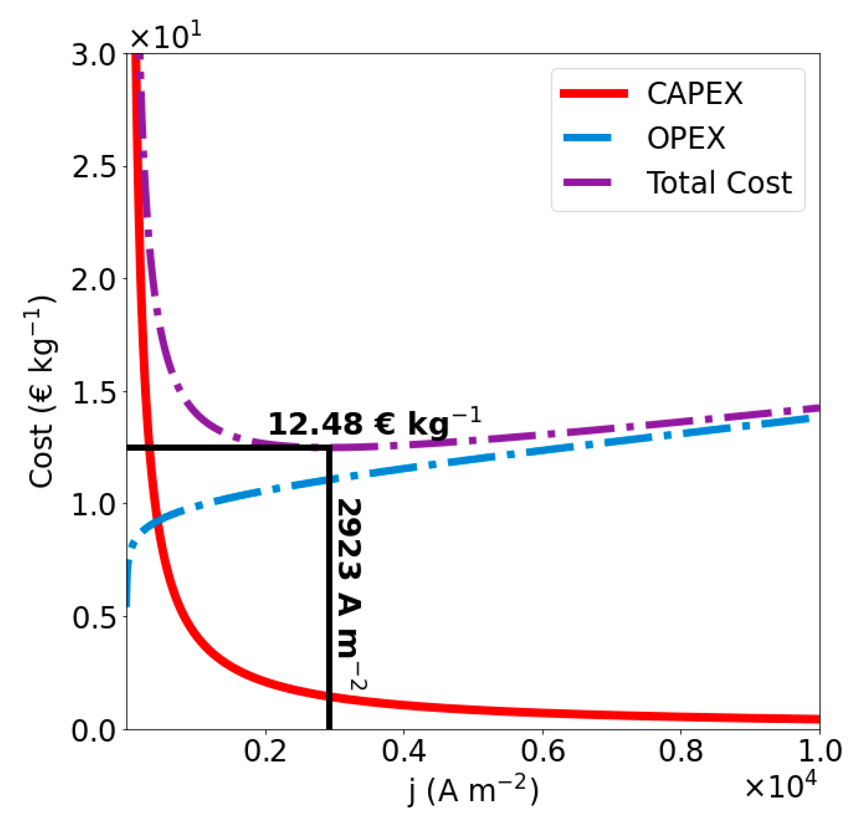
| (A m−2) | 2923 | 3214 | 1000 |
| (–) | 0.3 | 0.23 | 0.2 |
| (K) | 350 | 350 | 350 |
| (bar) | 1 | 1 | 1 |
| (€ kg−1) | 1.42 | 1.30 | 0.22 |
| (€ kg−1) | 11.06 | 11 | 9.85 |
| (€ kg−1) | 12.48 | 12.30 | 10.07 |
Publisher’s Note: MDPI stays neutral with regard to jurisdictional claims in published maps and institutional affiliations. |
© 2020 by the authors. Licensee MDPI, Basel, Switzerland. This article is an open access article distributed under the terms and conditions of the Creative Commons Attribution (CC BY) license (http://creativecommons.org/licenses/by/4.0/).
Share and Cite
Le Bideau, D.; Chocron, O.; Mandin, P.; Kiener, P.; Benbouzid, M.; Sellier, M.; Kim, M.; Ganci, F.; Inguanta, R. Evolutionary Design Optimization of an Alkaline Water Electrolysis Cell for Hydrogen Production. Appl. Sci. 2020, 10, 8425. https://doi.org/10.3390/app10238425
Le Bideau D, Chocron O, Mandin P, Kiener P, Benbouzid M, Sellier M, Kim M, Ganci F, Inguanta R. Evolutionary Design Optimization of an Alkaline Water Electrolysis Cell for Hydrogen Production. Applied Sciences. 2020; 10(23):8425. https://doi.org/10.3390/app10238425
Chicago/Turabian StyleLe Bideau, Damien, Olivier Chocron, Philippe Mandin, Patrice Kiener, Mohamed Benbouzid, Mathieu Sellier, Myeongsub Kim, Fabrizio Ganci, and Rosalinda Inguanta. 2020. "Evolutionary Design Optimization of an Alkaline Water Electrolysis Cell for Hydrogen Production" Applied Sciences 10, no. 23: 8425. https://doi.org/10.3390/app10238425