1. Introduction
Epidemiology—from the Greek epi (about), demos (people), and logos (study)—tries to study the distribution and determinant factors of diseases and applies this study to their control and prevention. It integrates procedures and techniques from disciplines such as the biomedical sciences and the social sciences [
1,
2,
3,
4]. One of the first works on the subject was proposed by Kermack and McKendrick in [
2] where an SIR (susceptible-infectious-recovered) epidemic model with the host population being split into three categories depending on the status of the individuals with respect to the disease was proposed. Multiple studies and investigations have been carried out, thus developing new variants of this model, such as SEIR (susceptible-exposed-infectious-recovered) or SIS (susceptible-infectious-susceptible) [
3,
4]. The use of mathematical models, epidemiological models, constitutes an essential part of epidemiology, as it is an excellent tool for the analysis and prediction of the spread of diseases. They also make it possible to simulate the practical consequences of different intervention and control measures—such as vaccination or partial or total quarantine interventions—and, thus, to determine the most appropriate strategy to be invoked depending on the epidemiological situation. From the mathematical point of view, the simplest epidemiological models are of deterministic nature and they are formulated using systems of either ordinary differential or in difference equations, where the independent variable is time. The epidemic mathematical models have been applied to study real infectious disease and they can be adequate, both in their structure and in their parameterization, to the particular disease under study. Particular examples of such a model adequacy are, for instance, Bombay’s epidemic pest of 1906 [
5], the current COVID-19 pandemic [
6,
7,
8], or measles and poliomyelitis [
9,
10]. In these two last cases, a periodic vaccination was proposed for a proportion of the susceptible based on an SIR epidemic model. Moreover, the strategy has been extended to impulsive periodic vaccination on more complex models, like for instance, SEIR models for cholera disease [
11], each with their corresponding disease-related parameterizations [
12].
The subpopulations under consideration usually change according to the model, but they always consist of groups or compartments into which the total population to be analyzed is divided. This work is only concerned with this type of model. However, there are different ways of formulating them, for example, considering the discrete time variable [
13] instead of continuous; involving systems of equations in differences; or introducing random elements, so that the model has stochastic dynamics [
14], which is a more realistic approach, but also more complicated to deal with. With regard to diseases, epidemiology deals with the modeling of infectious diseases—such as seasonal flu, chickenpox or the very recent COVID-19—even though epidemiological models are not limited only to this type of disease. However, it is in this case where development has been greatest in the last decades [
1] since the disease spread is a crucial factor in them, and epidemiological models offer a very good tool to deal with it.
In [
15,
16,
17,
18,
19], different types of vaccination strategies with eventual different application calendars and their achievable expected immunity are discussed. The fast and efficient tracking aspects of eventual infectious/susceptible infective contacts are examined in [
20,
21,
22,
23,
24,
25] in order to be able to achieve a prompt detection of new infective cases so as to try to avoid hospital collapse and a number of disease-related deaths. This concern has taken special relevance with the evolution of the current COVID-19 pandemic. The well-posedness of an epidemic model requires its fulfillment of basic properties like, for instance, the positivity of the solution under any non-negative initial conditions for any of the integrated subpopulations [
26] as expected, since one deals with a biological problem and its boundedness and stability for all time [
27,
28,
29,
30,
31], since the whole population in the habitat under study is bounded by nature. More recent studies on epidemic models have been developed in [
32] where fractional calculus is used to amend more basic epidemic models. Some recent SEIR models being parameterized and adapted for the description of the evolution of the COVID-19 pandemic have been considered in [
33,
34,
35,
36] and some references therein. In [
37,
38], Shannon’s information entropy is considered to study the transients in epidemic models focused on keeping the hospital availability of beds and hospital staff duties and other technical means below a certain admissible tolerance. See also some references therein. In [
39], a very general true-mass SEIR epidemic model is studied and tested under mixed regular and impulsive vaccination controls while keeping the needed properties of positivity and stability. In [
40,
41] and some references therein, stochastic epidemic models are described and analyzed subject to eventual altering noise on the nominal deterministic equilibrium steady-states. On the other hand, an SEIR epidemic normalized model under periodic impulsive vaccination is proposed and analyzed in [
42]. The initial simpler version of the model in the paper is assumed to be subject to a recruitment parameter, which is coincident with the natural mortality rate and the disease is assumed to be mortality-free. The dynamics of the recovered subpopulation are not considered in the analysis by taking advantage of the fact that the total population remains constant over time due to the absence of disease mortality. Afterwards, the model is generalized by incorporating a disease mortality rate. Furthermore, Floquet´s theory on stability of periodic solutions is involved in the proposed analysis without an explicit calculation of the Floquet´s eigenvalues which conform some of the given conditions for the stability of the periodic oscillations. It is also proven mathematically in the paper that, in some cases, the local asymptotic stability ensures the global one, and that the periodic impulsive vaccination is slightly more efficient than the continuous traditional strategy.
In this paper, the application of both the newborns and impulsive vaccination strategies in the SEIR model are studied. We reconsider the problem of an SEIR model under an additional specific disease mortality rate under vaccination of newborns, which can be interpreted as an ad hoc modification of the recruitment in the susceptible subpopulation. Such a vaccination effort can be optionally accommodated to the current amounts of susceptible subpopulation. The basic objective is to study the stability of the equilibrium solutions of the system—both in the case of newborn vaccination and in the case of impulsive vaccination—for the proposed model, which helps to understand their long-term behavior. Concerning the newborn vaccination, it is demonstrated, both analytically and numerically, that the proposed vaccination strategy can lead to the eradication of an endemic disease. The disease-free and the endemic equilibrium points are both characterized explicitly, their local asymptotic stability properties are formally discussed based on the calculation of the next generation matrix and its eigenvalues, and the reproduction number is explicitly linked to the vaccination effort. Furthermore, the instability (respectively, the stability) of the disease-free equilibrium point is seen to coincide with the attainability and stability (respectively, the non-attainability) of the endemic one. The local asymptotic stability is seen to also be global by combining properties of non-negativity of the solution with the values of Poincaré index for individual or groups of singular related to the discussion on the existence of limit cycles. Concretely, the local asymptotic stability is proven to also be global on the basis of the fact that the stable attainable attractor is the unique disease-free equilibrium point if reproduction number is less than unity (in which case the endemic equilibrium point is not attainable). Contrarily, if the disease-free equilibrium point is unstable, in the case of a reproduction number exceeding unity, then it is shown that it cannot be surrounded by a limit cycle in any of the phase planes; the only stable and attainable attractor being then the endemic equilibrium point. Another alternative vaccination strategy, which is also discussed in the paper under the same basic model, consists of a periodic impulsive vaccination. Again, the vaccination effort can be accommodated to the current stocks of susceptible subpopulation. The stability properties of the periodic steady-state are performed via Floquet´s theory, with an explicit calculation of the eigenvalues of the monodromy matrix which are the Floquet multipliers. This method allows us to establish that, under a sufficiently small transmission rate, the local asymptotic stability is guaranteed according to a formula which makes explicit a trade-off between the vaccination interval between consecutive vaccination pulses and the susceptible population fraction to be vaccinated by a defining a reproduction-like number. To perform the above summarized study, this work is split into five sections which are organized as follows.
Section 2 aims at establishing and discussing the SEIR model under eventual vaccination of newborns. The general formulation of the proposed SEIR model is given. Later on, the mathematical analysis of the model properties is discussed in detail in terms of local and global asymptotic stability concerns of both the disease-free and endemic equilibrium points, which are explicitly calculated as dependent of the vaccination of newborns levels. It is proven that the endemic equilibrium point is not reachable when the disease-free one is locally asymptotically stable, which happens as the basic reproduction number is less than unity. It is also proven that when the basic reproduction number exceeds unity then the endemic equilibrium point is reachable and locally asymptotically stable while the disease-free one is unstable. The reproduction number is improved with the levels of vaccination, which means that the reproduction number is kept below unity for wider ranges of potential values of the transmission rate as the vaccination effort increases. It is also proven that the local asymptotic stability of the equilibrium points also imply both respective global asymptotic stability properties. In the formulation of
Section 2, the absence of vaccination of newborns might be understood as a particular case of the corresponding vaccination effort. On the other hand, in
Section 3, an impulsive periodic vaccination strategy is proposed and studied, and the resulting model properties are formulated for the delay-free case. In this case, it is necessary to work with a resulting dynamic system of periodic coefficients, and, for this purpose, the Floquet theory is used to formulate the stability properties. Some numerical results are displayed and discussed in
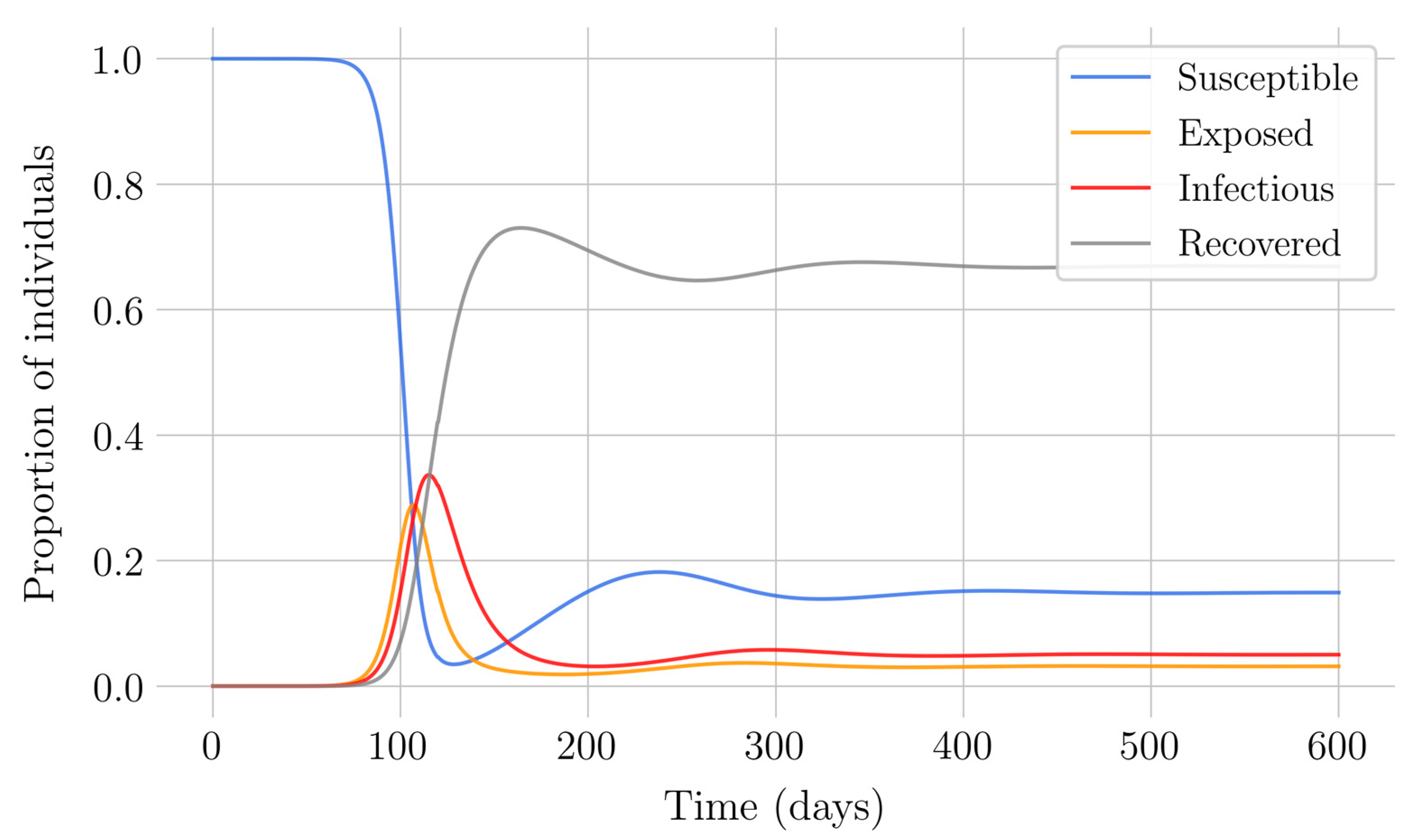
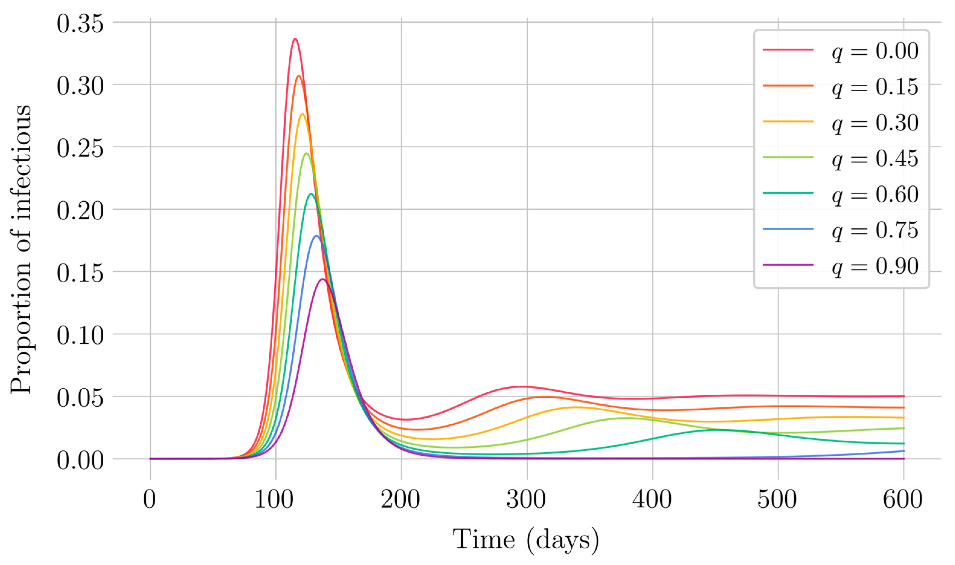
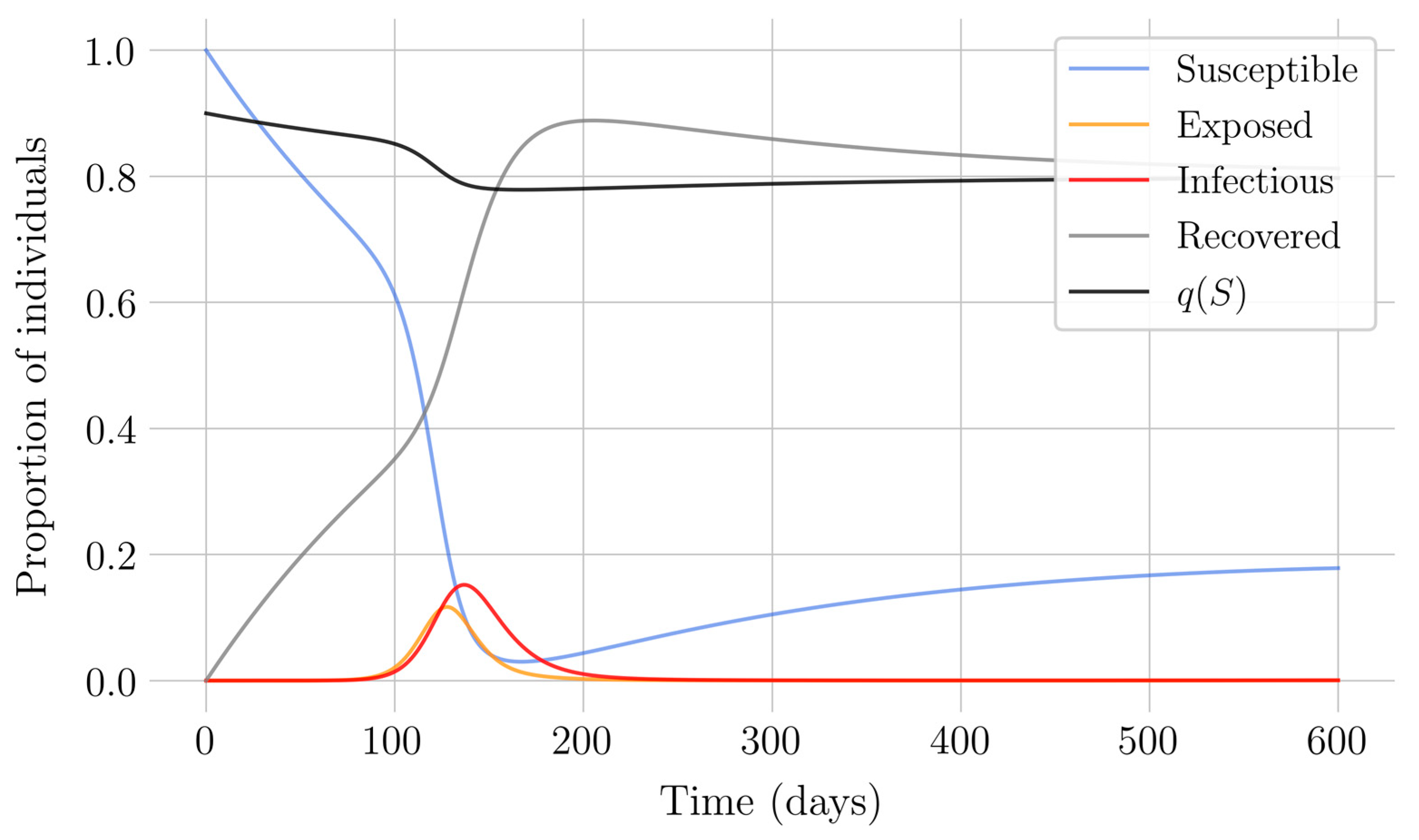
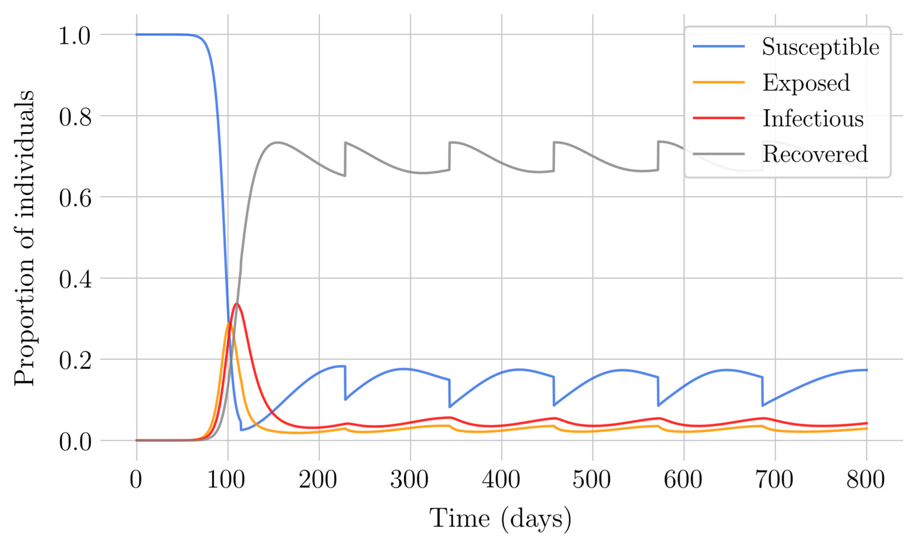
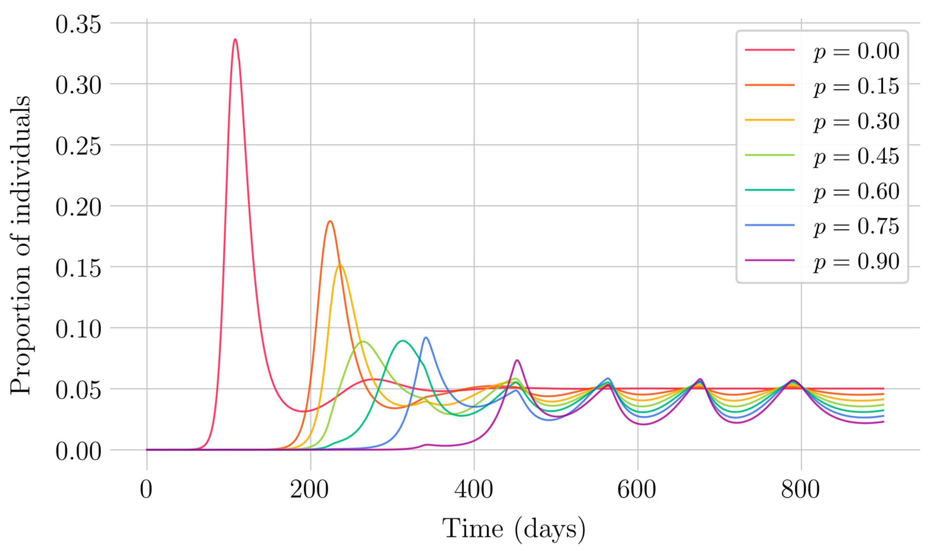
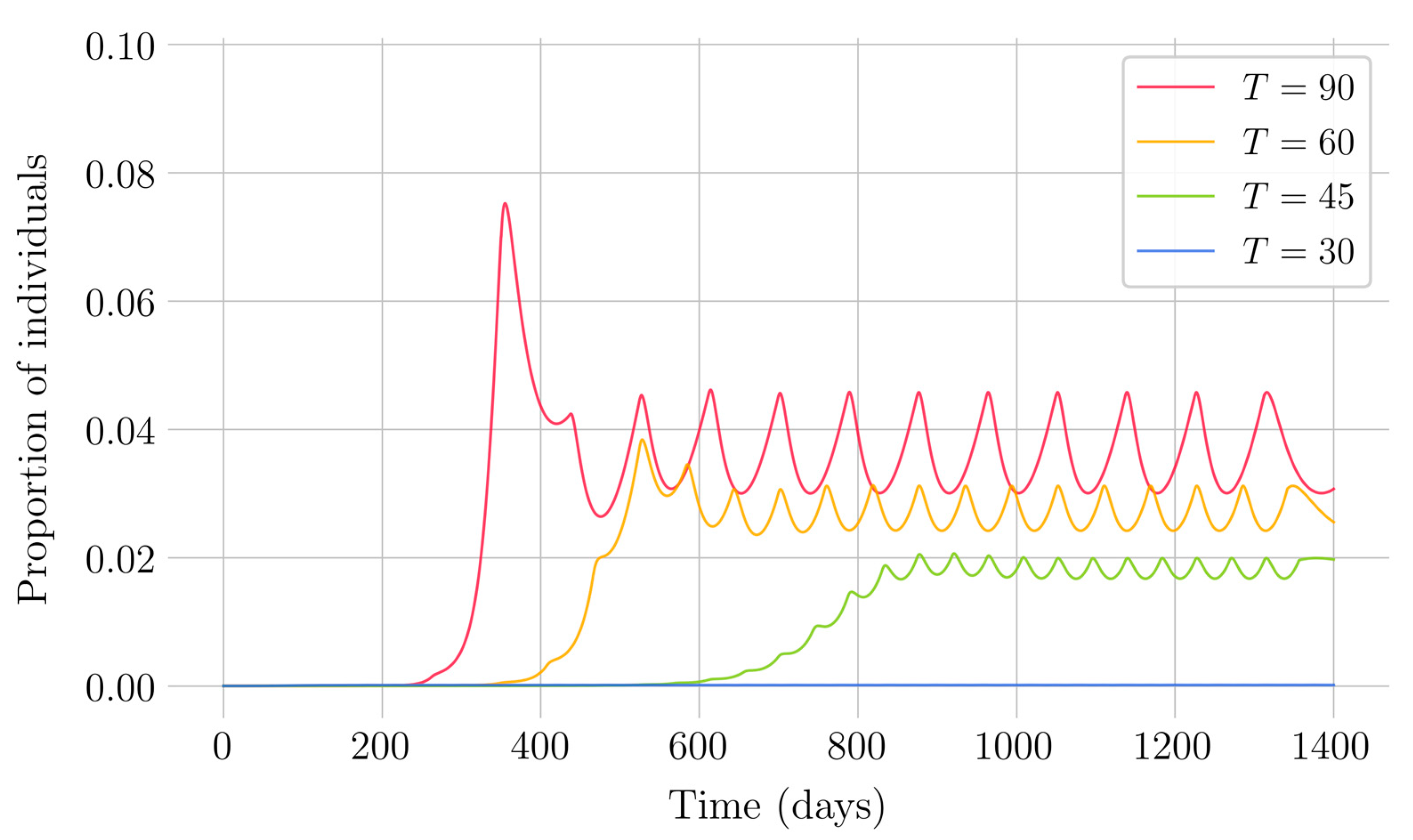
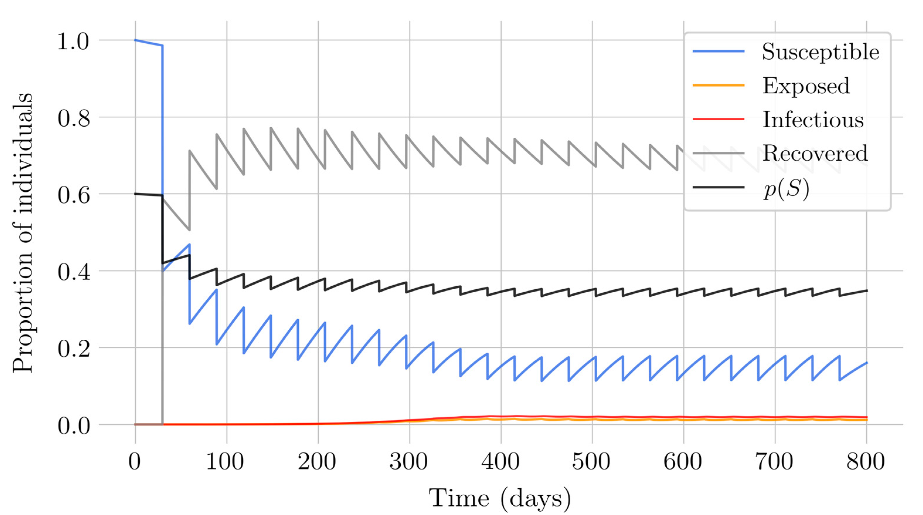
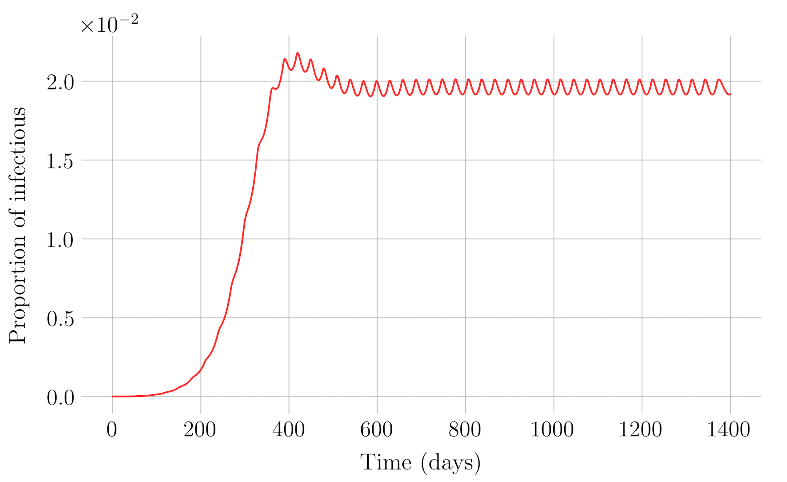
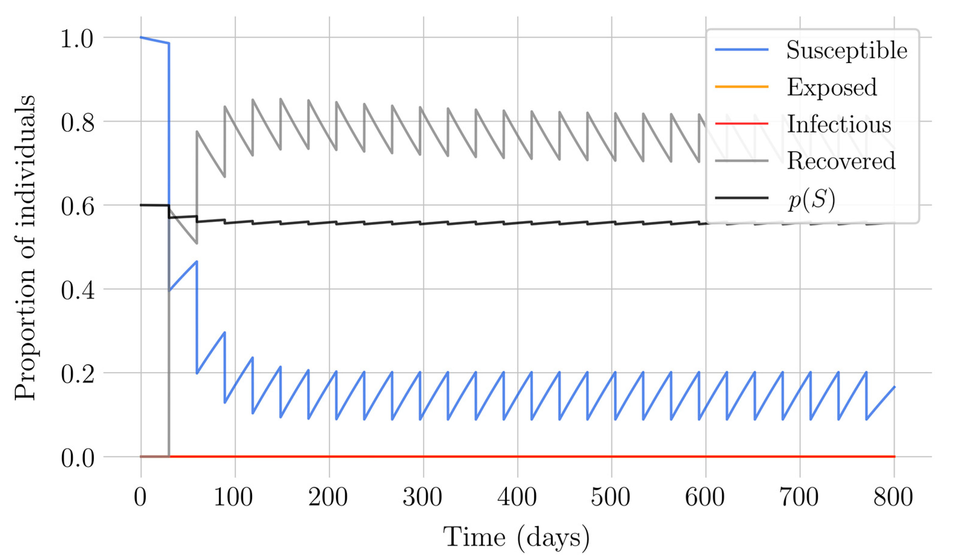
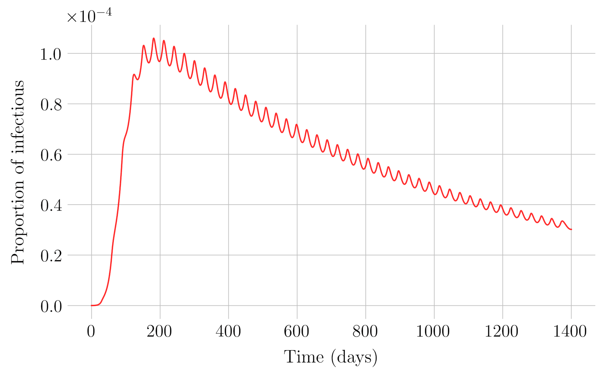
Section 4 for the COVID-19 pandemic, which are then performed to visualize the solutions for the two studied vaccination strategies. First, an endemic disease is simulated using the SEIR model, and then the mentioned vaccination strategies which are applied with the aim of eradicating the disease or, at least, softening its impact. To complete the section, two new control methods are designed by modifying the strategies presented by adapting them to the recruitment or susceptible levels in the sense that the control efforts are reinforced through time as such levels become larger. In this way, an attempt is made to propose new strategies that achieve eradication of the disease with less vaccination coverage, which is usually interesting in the context of the logistics of vaccination campaigns. The code for the programs developed for the simulations in this chapter has not been included in this report but can be found in the malenetxeberria/TFG-IngElec repository on GitHub. Finally, conclusions end the paper.
Compared to some related previous work, note that, in [
10], the pulse vaccination strategy is programmed on an SIR epidemic model while in the current paper, the impulsive periodic vaccination is proposed for an SEIR epidemic model. There are recent studies for COVID-19 concerns, see, for instance [
20,
21,
22,
23,
24,
25,
36]. However, those studies do not consider the potential application of vaccination which really does not yet exist in good condition for its mass application. Furthermore, most of the studies refer to short-term evaluations and prediction of the disease behavior. In the current work, two vaccination strategies are proposed for parameterizations associated to the COVID-19 pandemic. In particular, the second proposed strategy of periodic impulsive vaccination may be appropriate to deal with successive waves of serious incidence and later decrease of the infection. Furthermore, the vaccine administration strategies can be adapted to the levels of susceptible individuals which can facilitate the administration calendar.
2. SEIR Epidemic Model with Eventual Vaccination of Newborns
2.1. The Epidemic Model
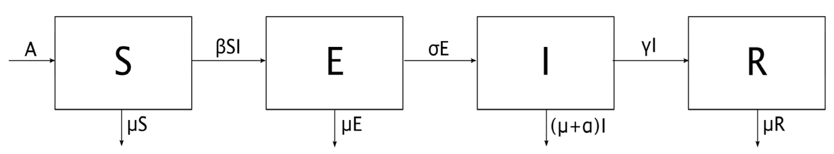
An SEIR epidemic model is proposed where the host population is split into four categories, namely:
- -
Susceptible: individuals who have not contracted the disease but are at risk for it, since they do not have the necessary antibodies to cope with it.
- -
Exposed: this is the group of individuals who are already infected, but who are not yet infectious, so they cannot transmit the infection. This state lasts for a limited period of time that varies according to the disease, and is known as the latent period [
1] (Chap. Two).
- -
Infectious: those individuals that are infected and can transmit the disease.
- -
Recovered: individuals who have managed to defeat the disease. The body generates immunity as an adaptive response to the infectious agent [
15], so that a recovered individual is no longer susceptible.
It is considered that the population is homogeneously mixed, that its spatial distribution is uniform, and that all susceptible individuals have the same probability of being infected, which simplifies the problem considerably. The mathematical representation of the SEIR model considered in this case [
3] is given by the system of differential equations:
subject to an initial condition given by:
S(0) ≥ 0,
E(0) ≥ 0,
I(0) ≥ 0 and
R(0) ≥ 0. The variables
S(
t),
E(
t),
I(
t), and
R(
t) indicate the proportion of susceptible, exposed, infectious, and recovered individuals of the subpopulations, with respect to the total population, found in each compartment at a specific time. The sum of the four subpopulations at the initial time instant is assumed to be unity, in general, so that the subpopulations of the model are fractions of the total initial population. However, this is not a real constraint since the initial conditions can be also fixed to the real values of the various subpopulations. The parameters are constant with positive values related to either demographic characteristics or to the infection type.
The symbols used for each variable or parameter are as follows:
S: Proportion of susceptible individuals
E: Proportion of exposed individuals
I: Proportion of infectious individuals
R: Proportion of recovered individuals
A: Proportion of new individuals per unit of time
β: Transmission rate
μ: Natural mortality rate
σ: Inverse of the latent period
γ: Recovery rate
α: Mortality rate caused by infection
q: Fraction of vaccinated newborns
Note the following facts on the above model:
New individuals enter the susceptible compartment per unit of time, either by birth or by immigration. βSI indicates the proportion of infections [
4], that is, the proportion of individuals who are no longer susceptible and who become exposed; and finally, μS is the proportion of individuals who die from causes not related to the infection, also per unit of time.
The infected susceptible βSI pass into the exposed compartment and are removed from it once the latent period has passed, that is, σE individuals are removed per unit of time. Naturally, the fraction μE of those exposed individuals who die from causes unrelated to infection must also be considered.
At the end of the latent period, the exposed σE become infectious. Moreover, γI is the proportion of individuals who overcome the disease and who, therefore, pass to the recovered compartment; instead, αI represents the individuals who die from the infection, and who are removed from the population.
γI individuals enter the recovered compartment per unit of time, and μR are withdrawn due to mortality from causes not related to the infection.
The fraction of vaccinated newborns is directly added to the recovered compartment and withdrawn from the susceptible one.
In this way, the scheme of the SEIR model is represented in
Figure 1.
2.2. Non-Negativity of the Solution
The solutions of Equation (1) are non-negative for all time for any given non-negative initial condition. This is easily proven by calculating, in a closed analytic form, the unique solution of Equation (1) for any set of non-negative initial conditions. This property is needed for well-posedness of the epidemic model Equation (1). In parallel, the fact that the total population is proven to be bounded for all time guarantees also the boundedness for all time of all the subpopulations under any given arbitrary finite non-negative initial conditions.
Theorem 1. The following properties hold for any:
- (i)
The solution trajectory of the epidemic model (1) is non-negative for all time for any given non-negative initial conditions.
- (ii)
The solution trajectory of Equation (1) is bounded for all time for any given finite non-negative initial conditions and. As a result, the epidemic model is globally stable for any given arbitrary finite non-negative initial conditions.
Proof. It is obvious that
for all time if
from the above first equation. Then,
for all time from the second equality of the above second equation if
,
, and
since
for all time. Subsequently,
for all time from the above third equation if
, since
for all time. Finally,
for all time from the above fourth equation if
, since
for all time. Property (i) has been proved. By summing-up the four subpopulations in Equation (1), one gets that the total population
satisfies the differential Equation (3)
whose solution is
so that the total population is bounded for all time. From Property (i), since all the subpopulations are non-negative for all time, it follows that they are also bounded for all time and that
for all time. In addition,
from the above equation. Furthermore
(otherwise, if
then
, a contradiction). Therefore,
. □
2.3. Equilibrium Points
There are two equilibrium points, that is, the disease-free one, which is obtained from (1) by equalizing to zero all the time-derivatives of Equation (1) and equalizing the infectious to zero. This leads to
On the other hand, the endemic equilibrium point is obtained from Equation (1) by equalizing again to zero all the time-derivatives while keeping a non-zero infectious subpopulation which yields:
where:
Recombining the above equations yields:
From Equation (5) into Equation (3) equalized to zero yields the total endemic equilibrium population:
Note that all the subpopulations of Equation (5), see also Equation (6), have to be non-negative for the endemic equilibrium point to exist in the first orthant of the state-space so that it be reachable. Otherwise, Theorem 1 would be violated. Thus, we have the subsequent result:
Proposition 1. The endemic equilibrium point is reachable if and only if the transmission rate is large enough to be non less than a critical value according to:for any.
If the transmission rate equalizes its critical value, then the endemic equilibrium point is coincident with the disease-free one. 2.4. Basic Reproduction Number and Stability of the Equilibrium Points
One of the most important parameters in epidemiology is the basic reproduction number
, which is defined as the average number of secondary cases caused by the entry of an infectious individual into a totally susceptible population [
1] (Chap. 2). There are several techniques for calculating the basic reproduction number, and in this work, the next generation method will be shown [
16], where
is the spectral radius of the next generation matrix. So, to build this matrix, first, one defines the transmission and transition function matrices
F and
–V defined from the second and third equations of (1) by:
which are evaluated at the disease-free equilibrium point to yield the matrix of dynamics of the linearized system around the disease-free equilibrium point, that is, the Jacobian matrix of the infective subsystem
at such a point,
Ref. [
38], where
is the identity matrix of second order. Since
is a stability matrix since the linearized system around the disease-free equilibrium point is globally asymptotically stable in the absence of disease, that is, if the transmission rate is zero, one follows from Equation (9) that
is a stability matrix if and only if the spectral radius of
is less than one or, equivalently, that of
that is
referred to as the basic reproduction number, is less than one, that is, if and only if
and this Jacobian matrix is critically stable for
and unstable for
. Comparing this result with Proposition 1, and since the eigenvalues of the Jacobian matrix Equation (9) of the infective pair (
E,
I) are continuous functions of the transmission rate, yields the result that the disease-free equilibrium point is asymptotically stable if and only if the endemic one is unreachable, which happens for a sufficiently small transmission rate as follows:
Theorem 2. The disease-free equilibrium point is the only reachable equilibrium point and it is globally asymptotically stable if and only if the transmission rate is small enough to satisfy. It is coincident with the endemic equilibrium point and critically stable ifand unstable if.
Proof. One has from the above discussion that for sufficiently close to the disease-free equilibrium point,
and
as
if
. On the other hand, note from Proposition 1 that, if
, then the exposed subpopulation is negative which contradicts Theorem 1(i). Therefore, the endemic equilibrium is not attainable if the reproduction number is less than one so that the only global stable attractor is the disease-free equilibrium point. On the other hand, all the subpopulations are bounded for all time and any
from Theorem 1. So that: (a) either
,
as
and the result is already proven; (b) at least one of
and
is unbounded as time increases, which is impossible since this unboundedness would contradict Theorem 1; (c) at least one of
and
exhibits asymptotic oscillations. However, then from the solutions in the proof of Theorem 1 and since
for all and
as :
therefore,
and
cannot oscillate asymptotically so that they converge to finite non-negative limits. Since the disease-free equilibrium point is unique, then
and
as
, and then the disease-free equilibrium point is (not only locally but also globally) asymptotically stable if and only if
. If
, then the spectral radius of the subsystem of the infective variables (
E,
I) exceeds unity so that the corresponding sub-matrix of the Jacobian matrix is unstable and then the whole Jacobian matrix at the disease-free equilibrium point is unstable. If
, then some eigenvalue of the Jacobian matrix of the disease-free equilibrium point is at the stability boundary and the linearized system is critically stable. □
Alternative proof. Consider the whole Jacobian matrix at the disease-free equilibrium point:
where
,
, and
. The eigenvalues of Equation (12) are
Note that
and
are real eigenvalues of the above Jacobian matrix. Then, the Jacobian matrix at the disease-free equilibrium point is a stability matrix if and only if
, that is, if and only if
which holds if and only if the transmission rate is small enough to satisfy
or, equivalently, if the basic reproduction number Equation (11) is less than one, equivalently
. If the inequality Equation (14), equivalently
, becomes an equality, still equivalent to
in (11), then
, that is, one eigenvalue of Equation (12) is critically stable and the disease-free equilibrium point is then critically stable. If the inequality in Equation (14) is reversed
then the disease-free equilibrium point is unstable.
Finally, note that the local asymptotic stability of the disease-free equilibrium point for is also global since:
- (a)
it is the unique attainable equilibrium point since the endemic one is not reachable from Proposition 1.
- (b)
the first right-hand-side term of Equation (2) tends asymptotically to zero as time tends to infinity so that, irrespective of the initial conditions, either the following limit exists:
which implies that the susceptible subpopulation tends to a finite and non-negative limit (from Theorem 1) as time tends to infinity, which is the disease-free equilibrium susceptible subpopulation. In this case, the (non-negative) integrand of the second term of the above limit tends asymptotically to zero; or
- (c)
it converges to a periodic solution of some period , that is, for some continuous as ; . □
If the image of is a real constant, then the convergence is to a point for all which is the susceptible component of the disease-free equilibrium point which is already discussed. If is not constant, then the susceptible subpopulation converges to a periodic solution. However, note that the second right-hand-side term of the first equation of (2) has a non-negative integrand so that either it converges to zero in order for S(t) to be bounded for all time or is asymptotically unbounded which violates Theorem 1. As a result, cannot exhibit an asymptotic oscillation while it converges to the disease-free susceptible equilibrium point as time tends to infinity.
Now, consider the two-dimensional phase plane at the disease-free susceptible equilibrium point . Since the reproduction number is less than one, the equilibrium point cannot be a saddle point, then its Poincaré index is +1 and no stable limit cycle can surround it. Thus, the disease-free equilibrium point, which is a local asymptotic attractor and the unique stable global attractor, is also the unique global asymptotic attractor if the reproduction number is less than one.
Remark 1. Note that, for any, the basic reproduction number in the case of vaccination of newborns becomes reduced tocompared to the case of absence of vaccination (whose corresponding reproduction number is), and then the disease-free equilibrium point is globally asymptotically stable if and only if. This implies that, under a vaccination of newborns effort, the global asymptotic stability of the disease-free equilibrium point together with the non-reachability of the endemic one are achieved if and only if Remark 2. An equivalent interpretation is that the stability of the disease-free equilibrium point and the parallel property of non-reachability of the endemic one are achievable for a larger range of transmission rate related to the absence of vaccination of newborns since the critical transmission rate satisfiesif(Proposition 1).
Remark 3. As a result of the above considerations, one can argue that vaccination of newborns effort is useful in achieving the asymptotic eradication of the disease since the range of transmission rate values being compatible with the stability of the disease-free equilibrium increases related to its parallel range of values in the absence of vaccination.
The subsequent result, whose proofs follow by direct calculation, relies on alternative equivalent expressions to Equation (6) on the components of the endemic equilibrium point depending on the reproduction number.
Proposition 2. The components of the endemic equilibrium point may be rewritten, equivalently to (6), as follows: It is reachable if and only ifand it is coincident with the disease-free equilibrium point if and only if.
Theorem 3. The endemic equilibrium point is globally asymptotically stable for anyif and only if the transmission rate satisfies, equivalently, if and only if the basic reproduction number exceeds unity.
Proof. The Jacobian matrix at the endemic equilibrium point is:
One of the eigenvalues of (16) is
. Instead of calculating the other three eigenvalues of Equation (16), which is a difficult task, the Routh–Hurwitz stability criterion
is applied to the characteristic equation of the third order remaining submatrix [
31], where
The Routh–Hurwitz criterion is applied by first calculating the following determinants:
The number of characteristic roots of
with positive real part is the number of sign changes in the set
. Since
and
, then there is no characteristic root with positive real part if and only if
[
28]. Note that
if and only if
, and
if and only if
which always holds. Then, (16) is a stability matrix if and only if
. Thus, the endemic equilibrium point is locally asymptotically stable if and only if
. It is now proven that such a stability property is global by using contradiction arguments. Assume that the solution is oscillatory periodic with some arbitrary oscillation period
. The period is supposed arbitrary since it is being rebutted by contradiction arguments in the following that some such oscillation period exits so that no limit oscillation exists as a result. Define
and
for the four subpopulations
. Note that all such claimed maximum values are positive real numbers. From Equation (2) in the proof of Theorem 1, one gets for
,
, and
that the limits below exist for any such a
:
after using the mean value theorem for integrals since all the involved integrals in Equation (2) are continuous functions of time. Note that
will define the periodic limit oscillation of the subpopulation
in the event that such an oscillation exists. By recombining the three first above equations, one gets for any given
, any
, and any supposed arbitrary oscillation period
that, since
for some
and any
:
which is violated if
Hence, a contradiction follows such that the exposed subpopulation does not have a limit oscillation of any potential oscillation period, since a chaotic behavior cannot exist either since the model has no small time-varying parameter. Similarly, one gets a similar conclusion on no existence of limit oscillations of any period of the infectious subpopulation since the oscillation condition is violated for a range of sufficiently small inter-period time instants for any arbitrary claimed oscillation period according to:
and similar conclusions can be deduced for the susceptible and the recovered individuals. Therefore, no limit cyclic exists surrounding the reachable endemic equilibrium point when the disease-free equilibrium point is unstable, that is, if the basic reproduction number exceeds unity. Furthermore, all solutions are bounded from Theorem 1. As a result, the endemic equilibrium point is globally asymptotically stable if the basic reproduction number exceeds unity, equivalently, if and only if
. □
Remark 4. It can be of interest to give some considerations which are based on known general results of the qualitative theory of differential equations which indicate that there is a unique global asymptotically stable attractor which is always one of the equilibrium points [43,44,45]. The global attractor is the disease-free equilibrium if the reproduction number is less than or equal to one and the endemic equilibrium point if such a parameter exceeds unity. In this way, there are no stable oscillations surrounding neither one of the equilibrium points nor jointly both of them. If the reproduction number is unity, then the asymptotic behavior is similar to that arising if it is less than unity so that the disease-free equilibrium point is a global asymptotically stable attractor. Thus, the constraints implying local asymptotic stability of any of the equilibrium points lead to their global asymptotic stability. Those considerations are deduced from the subsequent linked arguments: - (a)
If, then the disease-free equilibrium point is locally asymptotically stable and the endemic one is not reachable. A limit cycle surrounding it in any phase plane of two subpopulations, if any, would be unstable from the combined topology of equilibrium points and limit cycles. Therefore, it would be irrelevant for stability considerations. As a result, the disease-free equilibrium point is globally asymptotically stable (Theorem 2).
- (b)
If, then the endemic equilibrium point is locally asymptotically stable and the disease-free equilibrium point is unstable. A limit cycle surrounding it leaving away the disease-free one, if any, would be unstable for stability considerations. No limit cycles can exist surrounding both equilibrium points since the combined Poincaré index of both of them would be 0 (if the disease-free equilibrium point were a saddle point) or +2 (if the disease-free equilibrium point were not a saddle point). So, in any case, such a combined Poincaré index is not +1 compatible with the existence of some limit cycle surrounding both equilibrium points. As a result, the endemic equilibrium point is globally asymptotically stable if(Theorem 3).
- (c)
If, then the disease-free and the endemic equilibrium points are coincident. From the non-negativity property of the solution for any given non-negative initial conditions (Theorem 1 (i)), it follows that a limit cycle surrounding the equilibrium point cannot exist in the phase plane (E, I). Also, by inspection of (1), it follows thatandcan only have periodic asymptotic solutions ifandhave asymptotic periodic solutions. As a result, the stability is also asymptotic and global in this case.
5. Conclusions
In this work, the implementation of newborns and impulsive vaccination in the epidemiological model SEIR was studied. For this purpose, it was necessary to begin with an extensive theoretical framework in which the generalities of the model and the two vaccination strategies were explained, delving into some important concepts such as the existence and location of the equilibrium points or the state-steady periodic solutions and their stability properties, as well as their links to the ranges of values of the basic reproductive number. Although the central topic of the work is to study the influence of vaccination, it was considered important to devote a part of the paper body to these topics since feedback vaccination influences the allocation of the equilibrium states and the rates of convergence related to the absence of vaccination. In order to further study the vaccination model and control strategies, a part of the article has been devoted to stability analysis. In the case of newborn vaccination, the disease-free and endemic equilibrium points were found and Lyapunov’s first method was applied to verify their local stability properties. It was proven that the endemic equilibrium point is not reachable as the disease-free one is locally asymptotically stable while the endemic one is reachable as the disease-free one is unstable. Those facts also lead to the conclusion that the respective local stability properties are also global since any solution is bounded for finite non-negative initial conditions.
In the case of impulsive vaccination, the calculations were more involved due to the impulsive nature of the system. It can be argued that the impulsive vaccination strategy may be of particular relevant interest in endemic situations when the disease exhibits successive decreasing and increasing levels of infection through time. Instead of equilibrium points, periodic solutions are found and characterized and, due to the complexity of the problem, only the disease-free periodic solution was obtained. To demonstrate the local stability of the calculated solution, Floquet’s theory was applied, and in this way a stability condition containing an integral was obtained. Through some performed numerical simulations, it was possible to conclude, firstly, that both newborn and impulsive vaccination are effective strategies to eradicate the disease under sufficiently large levels of vaccination efforts. The required proportion of vaccination effort was seen to be relevant in both cases if the proportion of vaccines administered is proportional to the proportion of susceptible individuals. Secondly, it has been observed that the total coverage necessary to eradicate the disease was lower in the case of impulsive vaccination than in newborn vaccination, as mentioned in the theoretical framework. Regarding the strategy of impulsive vaccination, the local stability of a disease-free periodic solution was also demonstrated. Numerical simulations were developed by using background provided data for the disease parameterization of the SARS-COVID-19 pandemic. Although at this time there are no fully tested vaccines available for such a disease, the numerical examples adjusted to the formal setting indicate that the vaccination strategy improves the basic reproduction number and the disease is controlled more efficiently. It was also proven and tested through examples that the global vaccination strategy is better administrated if the vaccination effort is proportional to the susceptible subpopulation through time.


