Polarization Radiometric Calibration in Laboratory for a Channeled Spectropolarimeter

Abstract

The process of radiometric calibration would be coupled with the polarization properties of an optical system for spectropolarimetry, which would have significant influences on reconstructed Stokes parameters. In this paper, we propose a novel polarization radiometric calibration model that decouples the radiometric calibration coefficient and polarization properties of an optical system. The alignment errors of the polarization module and the variation of the retardations at different fields of view are considered and calibrated independently. According to these calibration results, the input Stokes parameters at different fields of view can be reconstructed accurately through the proposed model. Simulations are performed for the presented calibration and reconstruction methods, which indicate that the measurement accuracy of polarization information is improved compared with the traditional undecoupled calibration method.

1. Introduction

Imaging spectrometer and imaging polarimeter are of particular importance in many fields, including atmospheric aerosol characterization [1,2], remote sensing [3,4,5,6], and material characterization [7,8]. These fields require an imaging spectropolarimeter to simultaneously measure the spatial, spectral, and polarization information of a scene. In 1999, Oka and Iannarilli first described the channeled spectropolarimetry technique, an attractive approach for polarimetry [9,10] by which we can eliminate the disadvantages of conventional modulation principles. With a simple optical system and no movable polarization components, the entire wavelength-dependent state of polarization (SOP) and spectral information of a scene can be acquired simultaneously.

In recent publications, researchers have investigated incorporating the channeled spectropolarimetry technique into different types of imaging spectrometers, such as the dispersive imaging spectrometer [3,4,11], Fourier transform imaging spectrometer [6,12], and computed tomography imaging spectrometer [13,14]. Among these incorporations, the channeled spectropolarimetry technique with the dispersive imaging spectrometer, which is called the channeled dispersive imaging spectropolarimeter (CDISP), has a simple structure and is easier to implement in terms of technology. Noteworthy is that the CDISP should go through a series of accurate calibration before quantitative applications. For imaging instruments, the actual spectral radiance of the detected object should be obtained through radiometric calibration. For the imaging polarimeter, the target light from the detected object will be affected by the polarization properties of an optical system when transmitted in the optical system. This will change the polarimetric state of target light and affect the measurement accuracy of polarization information. Therefore, in the process of radiometric calibration for the imaging spectropolarimeter, the polarization properties of an optical system should be considered.

However, to the best of our knowledge, radiometric calibration for the imaging spectropolarimeter have not be well solved with the previous literature. Chunmin Zhang et al. implemented radiometric calibration and polarimetric calibration for the channeled interference imaging spectropolarimeter [15], while the two types of calibration are carried out separately. The radiometric calibration is the same as that of traditional imaging spectrometer, without taking into account the influence of the polarization properties of optical system. Michael W. Kudenov et al. provided the polarimetric calibration of the channeled polarimeter with a pushbroom hyperspectral imaging sensor only [4], without considering the radiometric calibration of the instrument. Bin Yang et al. presented a method of polarimetric calibration and reconstruction for the fieldable CDISP [16]. This method took into account the polarization properties of the optical system, but only if it can accurately measure the spectral radiance of the detected object.

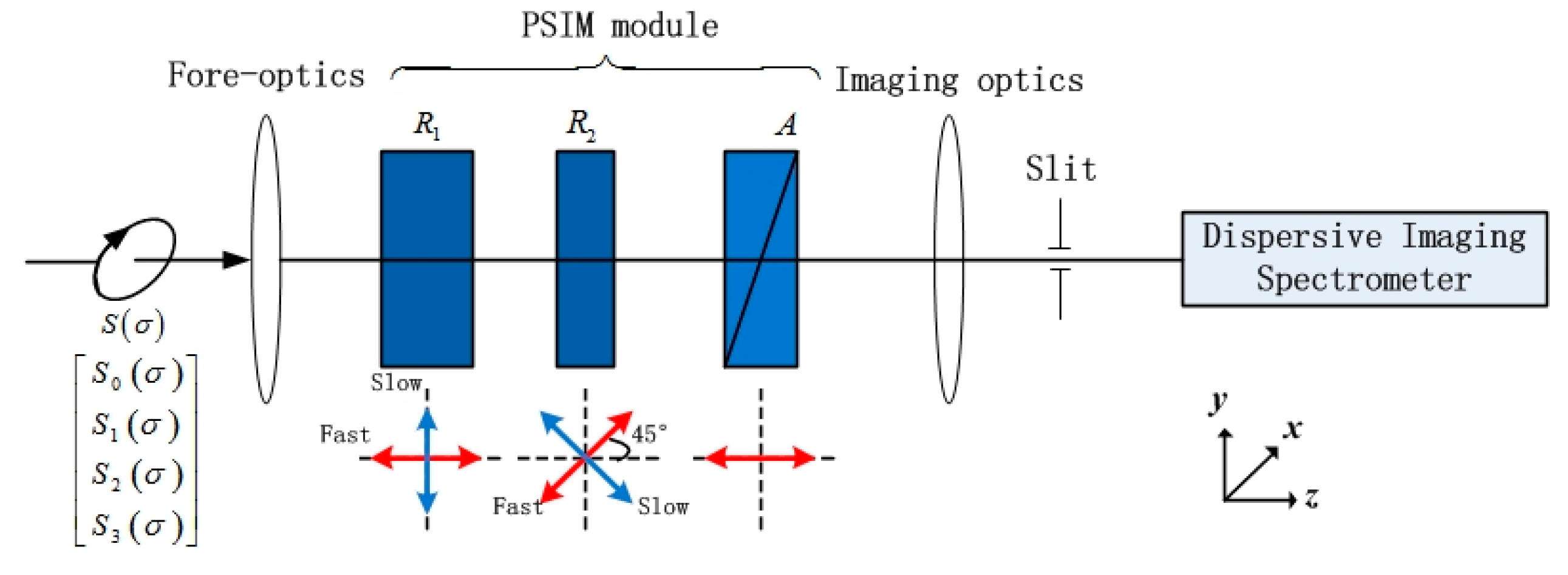
The interaction between the polarized beam and the optical system could be called polarization radiation transmission. Modeling and analyzing the polarization radiation transmission properties of optical system is the core to obtain the polarization properties of optical system and the theoretical basis for calibration of polarization detection system. In this paper, we use a fieldable CDISP designed for remote sensing as an example to analyze the influence of polarization properties of the optical system on radiometric calibration of the imaging spectropolarimeter. Considering simultaneously alignment errors of the polarimetric spectral intensity modulation (PSIM) module and variation of the retardations at different fields of view, we establish a polarization radiometric calibration model for the fieldable CDISP. Formerly, we proposed a model of self-correction with a 3:1 ratio of retarders to calibrate and compensate alignment errors and retardations simultaneously by measuring the SOP of target light in Ref. [17]. In order to maintain the advantages of this calibration method, the polarization radiometric calibration model proposed in this paper still adopts the scheme with a 3:1 ratio of retarders. Based on this model, we present a reconstruction method of Stokes parameters and a series of parameters calibration methods, classical radiometric calibration, self-correction technique, polarization radiometric decoupling calibration, and so on. By using the presented methods, the radiometric calibration coefficient and polarization parameters are determined accurately, and the reconstruction accuracy of the polarization information could be improved obviously, which is significant for the practical quantitative applications of the fieldable CDISP.

This paper is organized as follows. Section 2 provides the principle of fieldable channeled dispersive imaging spectropolarimetry, and then, derive a theoretical model for the polarization radiometric calibration and the reconstruction method of Stokes parameters. Section 3 proposes a series of calibration methods of parameters in the polarization radiometric calibration model. In Section 4, we analyze and summary our simulation experiment results. The conclusion is presented in Section 5.

2. Establishment of Polarization Radiometric Calibration Model of the Fieldable Channeled Dispersive Imaging Spectropolarimetry

In this section, we first introduce the principle of fieldable channeled dispersive imaging spectropolarimetry and its four sub-modules. Then, according to modularity theory and the principle of classical radiometric calibration, we derive a theoretical model for the polarization radiometric calibration.

2.1. Principle of the Fieldable Channeled Dispersive Imaging Spectropolarimetry

The optical schematic of the fieldable CDISP is depicted in Figure 1. In order to facilitate the establishment of polarization radiometric transmission model for optical system, we advanced a method modeling to divide into four sub-modules: fore-optics, PSIM module, imaging optics, and dispersive imaging spectrometer. Polarization information from a detected object is collected and collimated by the fore-optics, and then modulated by PSIM module. After passing though the imaging optics, the modulation spectrum is finally received by a dispersive imaging spectrometer. The fore-optics is used to meet the requirement that all incident angles on R₁ and R₂ are limited to less than about 5° in the PSIM module [3], and to reduce the size of polarization elements and the processing difficulty.

The PSIM module consists of two high-order retarders, R₁ and R₂, with thicknesses d₁ and d₂, respectively, and a linear analyzer, A. The fast axis of R₁ is aligned with the transmission axis of A, and R₂ is oriented with its fast axis at 45° to the transmission axis of A in an ideal condition. According to Mueller matrix theory and radiation transmission theory, if the incident Stokes vector is $S_{in}={\left[S_0,S_1,S_2,S_3\right]}^T$ (where T denotes the transpose operation), the Stokes vector of the target light passing through the PSIM module can be given by

$$S_{out}\left(\sigma \right)=M_{PSIM}\left(\sigma \right)\cdot S_{in}\left(\sigma \right)=M_A\left(0°\right)\cdot M_{R_2}\left[45°,{\phi }_2\left(\sigma \right)\right]\cdot M_{R_1}\left[0°,{\phi }_1\left(\sigma \right)\right]\cdot S_{in}\left(\sigma \right),$$

(1)

where $M_{R_2},$ and $M_{R_1}$ denote the Mueller matrices of A, R₂, and R₁, respectively [18], and ${\phi }_2\left(\sigma \right)$ and ${\phi }_1\left(\sigma \right)$ are the ideal phase retardations of R₂ and R₁, respectively. However, for a fieldable CDISP, ${\phi }_2\left(\sigma \right)$ and ${\phi }_1\left(\sigma \right)$ are related to the incident angle of the ray to the high-order retarders and will change with the increase of the field angle. In addition, alignment errors, ${\epsilon }_1$ and ${\epsilon }_2$ of R₁ and R₂, are inevitable for the manufacturing and alignment tolerances, which have significant influences on the reconstructed Stokes parameters. The Mueller matrix of the PSIM module becomes

$${M^{\prime }}_{PSIM}\left(\sigma ,\theta \right)={M^{\prime }}_P\left(0°,\sigma ,\theta \right)\cdot {M^{\prime }}_{R_2}\left[45°+{\epsilon }_2,{\phi }_2\left(\sigma ,\theta \right),\theta \right]\cdot {M^{\prime }}_{R_1}\left[{\epsilon }_1,{\phi }_1\left(\sigma ,\theta \right),\theta \right].$$

(2)

The polarization properties of optical system include diattenuation, retardance and depolarization. Thereinto, depolarization is intrinsically associated with scattering and a loss of coherence in the polarization state. A small amount of depolarization is associated with the scattered light from all optical components [18]. Therefore, only diattenuation and retardance were studied as the polarization properties of CDISP.

The fore-optics and imaging optics can be regarded as refractors. According to the Mueller matrix of each lens interface of optics and its series properties [18], the equivalent Mueller matrices of the fore-optics and imaging optics at the field of view θ can be expressed as

$$M_{fore}\left(\sigma ,\theta \right)=A_{fore}\left(\sigma ,\theta \right)\cdot \left[\begin{array}{cccc}1& D_{fore}\left(\sigma ,\theta \right)& 0& 0\\ D_{fore}\left(\sigma ,\theta \right)& 1& 0& 0\\ 0& 0& 1& {\delta }_{fore}\left(\sigma ,\theta \right)\\ 0& 0& -{\delta }_{fore}\left(\sigma ,\theta \right)& 1\end{array}\right],$$

(3)

$$M_{imag}\left(\sigma ,\theta \right)=A_{imag}\left(\sigma ,\theta \right)\cdot \left[\begin{array}{cccc}1& D_{imag}\left(\sigma ,\theta \right)& 0& 0\\ D_{imag}\left(\sigma ,\theta \right)& 1& 0& 0\\ 0& 0& 1& {\delta }_{imag}\left(\sigma ,\theta \right)\\ 0& 0& -{\delta }_{imag}\left(\sigma ,\theta \right)1\end{array}\right],$$

(4)

where $A_{fore}\left(\sigma ,\theta \right)$ and $A_{imag}\left(\sigma ,\theta \right)$ are the transmittance of the fore-optics and imaging optics, respectively. $D_{fore}\left(\sigma ,\theta \right)$ and $D_{imag}\left(\sigma ,\theta \right)$ are the diattenuation of the fore-optics and imaging optics, respectively. ${\delta }_{fore}\left(\sigma ,\theta \right)$ and ${\delta }_{imag}\left(\sigma ,\theta \right)$ are the retardance of the fore-optics and imaging optics, respectively.

Similarly, the dispersive imaging spectrometer can be regarded as a reflector, which is composed of many reflecting interfaces. The equivalent Mueller matrices at the field of view θ is given by

$$M_{spec}\left(\sigma ,\theta \right)=A_{spec}\left(\sigma ,\theta \right)\cdot \left[\begin{array}{cccc}1& D_{spec}\left(\sigma ,\theta \right)& 0& 0\\ D_{spec}\left(\sigma ,\theta \right)& 1& 0& 0\\ 0& 0& -1& -{\delta }_{spec}\left(\sigma ,\theta \right)\\ 0& 0& {\delta }_{spec}\left(\sigma ,\theta \right)& -1\end{array}\right],$$

(5)

where $A_{spec}\left(\sigma ,\theta \right)$, $D_{spec}\left(\sigma ,\theta \right)$ and ${\delta }_{spec}\left(\sigma ,\theta \right)$ are the transmittance, diattenuation and retardance of the dispersive imaging spectrometer, respectively. For the fieldable CDISP, these polarization properties increase with the increase of field angle, so they will affect the measurement results and can not be ignored. In this system, the slit is placed along the X-axis, and only the field of view in X-direction exists. The azimuth of incident plane of each viewing chief ray is a fixed value of 0°, not a variable. Therefore, the Mueller matrices of sub-module would not be affected by azimuth angle.

2.2. Establishment of Polarization Radiometric Calibration Model

According to the principle of classical radiometric calibration [19,20], the relationship between the digital number (DN) of CCD detector and the spectral radiance at entrance pupil in the actual operation of the instrument can be given by

$$\begin{array}{lll}DN\left(\sigma ,\theta \right)& =A\left(\sigma ,\theta \right)\cdot & M_{spec}\left(\sigma ,\theta \right)\cdot M_{imag}\left(\sigma ,\theta \right)\cdot {M^{\prime }}_{PSIM}\left(\sigma ,\theta \right)\cdot M_{fore}\left(\sigma ,\theta \right)\cdot S\left(\sigma \right)+C\left(\sigma ,\theta \right)\\ & =A^k\left(\sigma ,\theta \right)\cdot & B\left(\sigma ,\theta \right)+C\left(\sigma ,\theta \right)\\ & =A^k\left(\sigma ,\theta \right)\cdot & \{X_0\left(\sigma ,\theta \right)+b_1{c}_1{X}_{12}\left(\sigma ,\theta \right)\\ & & +\frac{1}{2}{b}_2{c}_2{X}_{12}\left(\sigma ,\theta \right)\left\{\exp \left[-i{\phi }_2\left(\sigma ,\theta \right)\right]+\exp \left[i{\phi }_2\left(\sigma ,\theta \right)\right]\right\}\\ & & -\frac{1}{4}{b}_2\left(1+c_1\right)X_{123}^{\ast }\left(\sigma ,\theta \right)\exp \left\{-i\left[{\phi }_1\left(\sigma ,\theta \right)-{\phi }_2\left(\sigma ,\theta \right)\right]\right\}\\ & & -\frac{1}{4}{b}_2\left(1+c_1\right)X_{123}\left(\sigma ,\theta \right)\exp \left\{i\left[{\phi }_1\left(\sigma ,\theta \right)-{\phi }_2\left(\sigma ,\theta \right)\right]\right\}\\ & & +\frac{1}{2}{b}_1{c}_2{X}_{123}^{\ast }\left(\sigma ,\theta \right)\exp \left[-i{\phi }_1\left(\sigma ,\theta \right)\right]\\ & & +\frac{1}{2}{b}_1{c}_2{X}_{123}\left(\sigma ,\theta \right)\exp \left[i{\phi }_1\left(\sigma ,\theta \right)\right]\\ & & +\frac{1}{4}{b}_2\left(1-c_1\right)X_{123}^{\ast }\left(\sigma ,\theta \right)exp\left\{-i\left[{\phi }_1\left(\sigma ,\theta \right)+{\phi }_2\left(\sigma ,\theta \right)\right]\right\}\\ & & +\frac{1}{4}{b}_2\left(1-c_1\right)X_{123}\left(\sigma ,\theta \right)exp\left\{i\left[{\phi }_1\left(\sigma ,\theta \right)+{\phi }_2\left(\sigma ,\theta \right)\right]\right\}\}+C\left(\sigma ,\theta \right),\end{array}$$

(6)

where $DN\left(\sigma ,\theta \right)$ is the original DN of the CCD detector, $A\left(\sigma ,\theta \right)$ represents the detector pixel response, and $C\left(\sigma ,\theta \right)$ is the DN of CCD dark current. For a dispersive spectropolarimeter, $\left(\sigma ,\theta \right)$ represents the positions of different pixels on the CCD detector. And

$$\begin{array}{l}{A}^k\left(\sigma ,\theta \right)=\frac{1}{2}{A}_{spec}\left(\sigma ,\theta \right)A_{imag}\left(\sigma ,\theta \right)A_{fore}\left(\sigma ,\theta \right)A\left(\sigma ,\theta \right)\\ \hspace{1em}\hspace{1em}\hspace{1em}\hspace{1em}\times \left[1+D_{spec}\left(\sigma ,\theta \right)+D_{imag}\left(\sigma ,\theta \right)+D_{spec}\left(\sigma ,\theta \right)D_{imag}\left(\sigma ,\theta \right)\right],\end{array}$$

(7)

is a function of the transmittance and diattenuation of sub-modules. Their values are different at different pixel positions of the CCD detector, that is, they change with the wavenumber and field of view. Therefore, we simply need to determine $A^k\left(\sigma ,\theta \right)$ with no need for determining the transmittance and diattenuation of sub-modules independently in the calibration. $A^k\left(\sigma ,\theta \right)$ is called radiometric calibration coefficient. Moreover $S\left(\sigma \right)={\left[S_0\left(\sigma \right),S_1\left(\sigma \right),S_2\left(\sigma \right),S_3\left(\sigma \right)\right]}^T$ is the spectral radiance at entrance pupil of the instrument. The spectral radiance at the entrance pupil, contains spectral, intensity and polarization information of the detected object, is modulated by the PSIM module into modulation spectrum. The modulation spectrum radiance could be obtained by radiometric calibration of the DN of CCD detector, which can be expressed as

$$\begin{array}{ll}B\left(\sigma ,\theta \right)=& X_0\left(\sigma ,\theta \right)+b_1{c}_1{X}_{12}\left(\sigma ,\theta \right)\\ & +\frac{1}{2}{b}_2{c}_2{X}_{12}\left(\sigma ,\theta \right)\left\{\exp \left[-i{\phi }_2\left(\sigma ,\theta \right)\right]+\exp \left[i{\phi }_2\left(\sigma ,\theta \right)\right]\right\}\\ & -\frac{1}{4}{b}_2\left(1+c_1\right)X_{123}^{\ast }\left(\sigma ,\theta \right)\exp \left\{-i\left[{\phi }_1\left(\sigma ,\theta \right)-{\phi }_2\left(\sigma ,\theta \right)\right]\right\}\\ & -\frac{1}{4}{b}_2\left(1+c_1\right)X_{123}\left(\sigma ,\theta \right)\exp \left\{i\left[{\phi }_1\left(\sigma ,\theta \right)-{\phi }_2\left(\sigma ,\theta \right)\right]\right\}\\ & +\frac{1}{2}{b}_1{c}_2{X}_{123}^{\ast }\left(\sigma ,\theta \right)\exp \left[-i{\phi }_1\left(\sigma ,\theta \right)\right]\\ & +\frac{1}{2}{b}_1{c}_2{X}_{123}\left(\sigma ,\theta \right)\exp \left[i{\phi }_1\left(\sigma ,\theta \right)\right]\\ & +\frac{1}{4}{b}_2\left(1-c_1\right)X_{123}^{\ast }\left(\sigma ,\theta \right)exp\left\{-i\left[{\phi }_1\left(\sigma ,\theta \right)+{\phi }_2\left(\sigma ,\theta \right)\right]\right\}\\ & +\frac{1}{4}{b}_2\left(1-c_1\right)X_{123}\left(\sigma ,\theta \right)exp\left\{i\left[{\phi }_1\left(\sigma ,\theta \right)+{\phi }_2\left(\sigma ,\theta \right)\right]\right\},\end{array}$$

(8)

where

$$\{\begin{array}{l}{a}_1=\sin 2{\epsilon }_1\\ a_2=\cos 2{\epsilon }_1\end{array},\{\begin{array}{l}{b}_1=\sin 2{\epsilon }_2\\ b_2=\cos 2{\epsilon }_2\end{array},\{\begin{array}{l}{c}_1=\sin 2\left({\epsilon }_2-{\epsilon }_1\right)\\ c_2=\cos 2\left({\epsilon }_2-{\epsilon }_1\right)\end{array},$$

(9)

$$\{\begin{array}{l}\hspace{1em}\hspace{1em}{X}_0\left(\sigma ,\theta \right)=S_0\left(\sigma \right)+D_{fore}\left(\sigma ,\theta \right)S_1\left(\sigma \right)\\ \hspace{1em}\hspace{1em}{X}_1\left(\sigma ,\theta \right)=D_{fore}\left(\sigma ,\theta \right)S_0\left(\sigma \right)+S_1\left(\sigma \right)\\ \hspace{1em}\hspace{1em}{X}_2\left(\sigma ,\theta \right)=S_2\left(\sigma \right)+{\delta }_{fore}\left(\sigma ,\theta \right)S_3\left(\sigma \right)\\ \hspace{1em}\hspace{1em}{X}_3\left(\sigma ,\theta \right)=S_3\left(\sigma \right)-{\delta }_{fore}\left(\sigma ,\theta \right)S_2\left(\sigma \right)\\ \hspace{1em}\hspace{1em}{X}_{12}\left(\sigma ,\theta \right)=a_2{X}_1\left(\sigma ,\theta \right)+a_1{X}_2\left(\sigma ,\theta \right)\\ X_{123}\left(\sigma ,\theta \right)=a_1{X}_1\left(\sigma ,\theta \right)-a_2{X}_2\left(\sigma ,\theta \right)+i{X}_3\left(\sigma ,\theta \right)\end{array},$$

(10)

and the superscript $\ast$ denotes the complex conjugate.

Based on Equation (8), the nine phase terms represent nine distinct channels in Fourier domain which contain the data related to the input Stokes parameters $S_0\left(\sigma \right),$ $S_1\left(\sigma \right),$ and $S_3\left(\sigma \right).$ Calculating the autocorrelation of $B\left(\sigma ,\theta \right)$ using the Fourier transformation, we can distribute the nine channels with nine phase terms

$$\begin{array}{ll}{C}^{\theta }\left(L\right)& =C_0^{\theta }\left(L\right)+C_1^{\theta }\left(L-L_2\right)+C_{-1}^{\theta }\left(-L-L_2\right)\\ & +C_2^{\theta }\left[L-\left(L_1-L_2\right)\right]+C_{-2}^{\theta }\left[-L-\left(L_1-L_2\right)\right]\\ & +C_3^{\theta }\left(L-L_1\right)+C_{-3}^{\theta }\left(-L-L_1\right)\\ & +C_4^{\theta }\left[L-\left(L_1+L_2\right)\right]+C_{-4}^{\theta }\left[-L-\left(L_1+L_2\right)\right],\end{array}$$

(11)

where L denotes the variable conjugate to wavenumber σ under the Fourier transform, and the superscript $\theta$ is the field angle. $L_j=\Delta n\left(\sigma \right)d_j,$ is the optical path difference (OPD) introduced by R_j, $\Delta n\left(\sigma \right)$ is the birefringence of the birefringent crystal. By filtering out nine channels and performing inverse Fourier transformations independently, the whole Stokes parameters of the target light can be described as

$$S_0\left(\sigma \right)=\frac{X_0\left(\sigma ,\theta \right)-D_{fore}\left(\sigma ,\theta \right)X_1\left(\sigma ,\theta \right)}{1-D_{fore}^2\left(\sigma ,\theta \right)},$$

(12)

$$S_1\left(\sigma \right)=\frac{X_1\left(\sigma ,\theta \right)-D_{fore}\left(\sigma ,\theta \right)X_0\left(\sigma ,\theta \right)}{1-D_{fore}^2\left(\sigma ,\theta \right)},$$

(13)

$$S_2\left(\sigma \right)=\frac{X_2\left(\sigma ,\theta \right)-{\delta }_{fore}\left(\sigma ,\theta \right)X_3\left(\sigma ,\theta \right)}{1+{\delta }_{fore}^2\left(\sigma ,\theta \right)},$$

(14)

$$S_3\left(\sigma \right)=\frac{X_3\left(\sigma ,\theta \right)+{\delta }_{fore}\left(\sigma ,\theta \right)X_2\left(\sigma ,\theta \right)}{1+{\delta }_{fore}^2\left(\sigma ,\theta \right)},$$

(15)

where $X_i\left(\sigma ,\theta \right)$ can be obtained by reference to the self-correction method. The interested reader can find more information in [17].

From Equation (6), we can find that the polarization properties of imaging optics and dispersive imaging spectrometer will not influence the measurement of the CDISP. The process of measuring polarization information is complicated due to diattenuation and retardance of the fore-optics, $D_{fore}\left(\sigma ,\theta \right)$ and ${\delta }_{fore}\left(\sigma ,\theta \right).$ In addition, this effect will be more serious with the increase of field angle. However, the fore-optics is indispensable because of its important role in the fieldable CDISP [16], so we need to calibrate the polarization properties of fore-optics accurately. Based on the derived theoretical model, the parameters, $A^k\left(\sigma ,\theta \right),$ $C\left(\sigma ,\theta \right),$ ${\epsilon }_1,$ ${\epsilon }_2,$ $\exp \left[i{\phi }_2\left(\sigma \right)\right],$ $\exp \left\{-i\left[{\phi }_1\left(\sigma ,\theta \right)+{\phi }_2\left(\sigma \right)\right]\right\},$ $D_{fore}\left(\sigma ,\theta \right)$, and ${\delta }_{fore}\left(\sigma ,\theta \right),$ are needed to be calibrated accurately to reconstruct the Stokes parameters accurately.

3. Method of Polarization Radiometric Calibration

In the presented methods, we proposed a series of calibration methods of parameters in the polarization radiometric calibration model. We first briefly expound the classical radiometric calibration method to obtain the dark current response $C\left(\sigma ,\theta \right)$ and modulated radiometric calibration coefficient $A^{k^{\prime }}\left(\sigma ,\theta \right).$ Then the polarization parameters independent of field of view are calibrated with self-correction technique. Different from the radiometric calibration of traditional imaging spectrometer, the radiometric calibration coefficient and polarization parameters would be coupled in the calibration process for the fieldable CDISP. Therefore, we come up with a polarization radiometric decoupling calibration method to achieve the accurate calibration of the radiometric calibration coefficient $A^k\left(\sigma ,\theta \right)$ and diattenuation of fore-optics $D_{fore}\left(\sigma ,\theta \right)$. Finally, $\exp \left\{-i\left[{\phi }_1\left(\sigma ,\theta \right)+{\phi }_2\left(\sigma \right)\right]\right\}$ and ${\delta }_{fore}\left(\sigma ,\theta \right)$ are acquired by using the 0° and 45° linearly polarized reference beam.

3.1. Classical Radiometric Calibration

According to the classical radiometric calibration method [19], the dark current response $C\left(\sigma ,\theta \right)$ and modulated radiometric calibration coefficient $A^{k^{\prime }}\left(\sigma ,\theta \right)$ can be calibrated by using the lights generated by integrating sphere. The integrating sphere provides unpolarized polychromatic lights that $S_0\left(\sigma \right)\ne 0,$$S_1\left(\sigma \right)=0,$$S_2\left(\sigma \right)=0,$ and $S_3\left(\sigma \right)=0$. Substituting these equations into Equation (6), we know that, due to the existence of polarization properties, the calibrated $A^{k^{\prime }}\left(\sigma ,\theta \right)$ is not $A^k\left(\sigma ,\theta \right)$ as we needed, but the result of its coupling with the polarization parameters. $A^{k^{\prime }}\left(\sigma ,\theta \right)$ is given by

$$\begin{array}{l}{A}^k{}^{\prime }\left(\sigma ,\theta \right)=A^k\left(\sigma ,\theta \right)\cdot \{1+a_2{b}_1{c}_1{D}_{fore}\left(\sigma ,\theta \right)\\ \hspace{1em}\hspace{1em}\hspace{1em}+\frac{1}{2}{a}_2{b}_2{c}_2{D}_{fore}\left(\sigma ,\theta \right)\left\{\exp \left[-i{\phi }_2\left(\sigma \right)\right]+\exp \left[i{\phi }_2\left(\sigma \right)\right]\right\}\\ \hspace{1em}\hspace{1em}\hspace{1em}-\frac{1}{4}{a}_1{b}_2\left(1+c_1\right)D_{fore}\left(\sigma ,\theta \right)\exp \left\{-i\left[{\phi }_1\left(\sigma ,\theta \right)-{\phi }_2\left(\sigma \right)\right]\right\}\\ \hspace{1em}\hspace{1em}\hspace{1em}-\frac{1}{4}{a}_1{b}_2\left(1+c_1\right)D_{fore}\left(\sigma ,\theta \right)\exp \left\{i\left[{\phi }_1\left(\sigma ,\theta \right)-{\phi }_2\left(\sigma \right)\right]\right\}\\ \hspace{1em}\hspace{1em}\hspace{1em}+\frac{1}{2}{a}_1{b}_1{c}_2{D}_{fore}\left(\sigma ,\theta \right)\left\{\exp \left[-i{\phi }_1\left(\sigma ,\theta \right)\right]+\exp \left[i{\phi }_1\left(\sigma ,\theta \right)\right]\right\}\\ \hspace{1em}\hspace{1em}\hspace{1em}+\frac{1}{4}{a}_1{b}_2\left(1-c_1\right)D_{fore}\left(\sigma ,\theta \right)\exp \left\{-i\left[{\phi }_1\left(\sigma ,\theta \right)+{\phi }_2\left(\sigma \right)\right]\right\}\\ \hspace{1em}\hspace{1em}\hspace{1em}+\frac{1}{4}{a}_1{b}_2\left(1-c_1\right)D_{fore}\left(\sigma ,\theta \right)\exp \left\{i\left[{\phi }_1\left(\sigma ,\theta \right)+{\phi }_2\left(\sigma \right)\right]\right\}\}\end{array}$$

(16)

Based on Equation (16), the radiometric calibration coefficient is coupled with the polarization properties in the process of radiometric calibration for fieldable CDISP. It is necessary to decouple them to achieve accurate polarization radiometric calibration. Before decoupling them, the basic polarization parameters need to be calibrated.

3.2. Self-Correction of Alignment Errors ${\epsilon }_1,$${\epsilon }_2$ and Retardation $\exp \left[i{\phi }_2\left(\sigma \right)\right]$

The alignment errors of two high-order retarders do not change with the field of view. In addition, the variation of the phase retardation of R₂ with the field of view is too small, so that it can be ignored [16], so we can use the value of ${\phi }_2\left(\sigma \right)$ at the central fields of view (FOV) as the values of the entire FOV. At central FOV, the beam light is incident vertically to the interface of each lens of fore-optics, so its polarization properties can be negligible, $D_{fore}^{}\left(\sigma ,0\right)\approx 0$ and ${\delta }_{fore}^{}\left(\sigma ,0\right)\approx 0$. Substituting these into the Equation (16), we obtain that $A^k\left(\sigma ,0\right)=A^{k^{\prime }}\left(\sigma ,0\right).$ Therefore, the modulated radiometric calibration coefficient of central FOV can be used to acquire the modulation spectrum radiance after passing the PSIM module. Based on the calibrated modulation spectrum radiance, the above polarization parameters, ${\epsilon }_1,$${\epsilon }_2,$ and $\exp \left[i{\phi }_2\left(\sigma \right)\right],$ can be obtained by using the self-correction method [17].

3.3. Decoupling of Radiation Calibration Coefficient $A^k\left(\sigma ,\theta \right)$ and Diattenuation of Fore-Optics $D_{fore}\left(\sigma ,\theta \right)$

In the process of radiometric calibration, calibration coefficient $A^k\left(\sigma ,\theta \right)$ and polarization property $D_{fore}\left(\sigma ,\theta \right)$ are modulated to different frequencies by two high-order retarders. The Fourier transformation of $A^{k^{\prime }}\left(\sigma ,\theta \right)$ gives the autocorrelation function, which can be expressed as

$$\begin{array}{ll}{G}^{\theta }\left(L\right)& =G_0^{\theta }\left(L\right)+G_1^{\theta }\left(L-L_2\right)+G_{-1}^{\theta }\left(-L-L_2\right)\\ & +G_2^{\theta }\left[L-\left(L_1-L_2\right)\right]+G_{-2}^{\theta }\left[-L-\left(L_1-L_2\right)\right]\\ & +G_3^{\theta }\left(L-L_1\right)+G_{-3}^{\theta }\left(-L-L_1\right)\\ & +G_4^{\theta }\left[L-\left(L_1+L_2\right)\right]+G_{-4}^{\theta }\left[-L-\left(L_1+L_2\right)\right].\end{array}$$

(17)

By filtering out the desired channels and performing inverse Fourier transformations independently, the radiometric calibration coefficient $A^k\left(\sigma ,\theta \right)$ and diattenuation of fore-optics $D_{fore}\left(\sigma ,\theta \right)$ can be described as

$$D_{fore}\left(\sigma ,\theta \right)=\frac{2{ℱ}^{-1}\left\{G_1{}^{\theta }\right\}}{a_2{b}_2{c}_2{ℱ}^{-1}\left\{G_0{}^{\theta }\right\}\exp \left[-i{\phi }_2\left(\sigma \right)\right]-2a_2{b}_1{c}_1{ℱ}^{-1}\left\{G_1{}^{\theta }\right\}},$$

(18)

$$A^k\left(\sigma ,\theta \right)=2{ℱ}^{-1}\left\{G_0{}^{\theta }\right\}-2\frac{b_1{c}_1}{b_2{c}_2}2{ℱ}^{-1}\left\{G_1{}^{\theta }\right\}\exp \left[i{\phi }_2\left(\sigma \right)\right],$$

(19)

where $a_i,$ $b_i,$ and $c_i$ can be computed through ${\epsilon }_1$ and ${\epsilon }_2$ calibrated in Section 3.2, and $\exp \left[i{\phi }_2\left(\sigma \right)\right]$ as computed in Section 3.2.

For the traditional imaging spectropolarimeter, the influence of polarization properties of optical system on radiometric calibration is not considered. $A^{k^{\prime }}\left(\sigma ,\theta \right)$ is directly taken as the radiometric calibration coefficient, so that there is a deviation between the spectral radiance obtained by calibration and the spectral radiance at the entrance pupil.

3.4. Calibration of Retardation $\exp \left\{-i\left[{\phi }_1\left(\sigma ,\theta \right)+{\phi }_2\left(\sigma \right)\right]\right\}$ and Retardance of Fore-Optics ${\delta }_{fore}\left(\sigma ,\theta \right)$

The variation of the phase retardation of R₁ with the field of view will significantly influence the measurement accuracy of the fieldable CDISP [16], so ${\phi }_1\left(\sigma ,\theta \right)$ cannot be regarded as a constant across the entire FOV. In addition, because the phase retardations of R₁ is always in the form of $\exp \left\{-i\left[{\phi }_1\left(\sigma ,\theta \right)+{\phi }_2\left(\sigma \right)\right]\right\}$ in the calibration and reconstruction of Stokes parameters, we just need to calibrate $\exp \left\{-i\left[{\phi }_1\left(\sigma ,\theta \right)+{\phi }_2\left(\sigma \right)\right]\right\}$.

To calibrate $\exp \left\{-i\left[{\phi }_1\left(\sigma ,\theta \right)+{\phi }_2\left(\sigma \right)\right]\right\}$ with the change of field angle, a 0° linearly polarized beam is entered into the system and filled the entire entrance pupil. For a 0° linearly polarized beam, $S_0\left(\sigma \right)=S_1\left(\sigma \right),$ $S_2\left(\sigma \right)=0,$ and $S_3\left(\sigma \right)=0$. 0 and the 4 channels in Equation (11) then become

$$C_{0,0°}^{\theta }=ℱ\left\{X_0\left(\sigma ,\theta \right)+a_2{b}_1{c}_1{X}_1\left(\sigma ,\theta \right)\right\},$$

(20)

$$C_{4,0°}^{\theta }=ℱ\{\frac{1}{4}{a}_1{b}_2(1-c_1)X_1\left(\sigma ,\theta \right)\exp \left\{-i\left[{\phi }_1\left(\sigma ,\theta \right)+{\phi }_2\left(\sigma \right)\right]\right\}\},$$

(21)

where $C_{0,0°}^{\theta }$ and $C_{4,0°}^{\theta }$ denote the channels obtained when the 0° linearly polarized beam is entered into entire entrance pupil of the instrument. By filtering out the desired channels and performing inverse Fourier transformations independently, $\exp \left\{-i\left[{\phi }_1\left(\sigma ,\theta \right)+{\phi }_2\left(\sigma \right)\right]\right\}$ can be described as

$$\exp \left\{-i\left[{\phi }_1\left(\sigma ,\theta \right)+{\phi }_2\left(\sigma \right)\right]\right\}=\frac{4\left(1+a_2{b}_1{c}_1\right)}{a_1{b}_2\left(1-c_1\right)}\cdot \frac{{ℱ}^{-1}\left\{C_{0,0°}^{\theta }\right\}}{{ℱ}^{-1}\left\{C_{4,0°}^{\theta }\right\}}.$$

(22)

For the fieldable CDISP, the polarization properties caused by the fore-optics is more serious with the increase of the field angle. The retardance of fore-optics, is different with the change of field angle. To calibrate ${\delta }_{fore}\left(\sigma ,\theta \right),$ a 45° linearly polarized beam is entered into the system and filled the entire entrance pupil. For a 45° linearly polarized beam, $S_0\left(\sigma \right)=S_2\left(\sigma \right),$ $S_1\left(\sigma \right)=0,$ and $S_3\left(\sigma \right)=0,$ Substituting these equations into Equation (11), we can obtain

$$C_{0,45°}^{\theta }=ℱ\left\{S_0\left(\sigma \right)+b_1{c}_1\left[a_2{D}_{fore}\left(\sigma ,\theta \right)S_0\left(\sigma \right)+a_1{S}_2\left(\sigma \right)\right]\right\},$$

(23)

$$\begin{gathered} C_{0,45°}^{\theta }=ℱ\{\frac{1}{4}{b}_2(1-c_1)[a_1{D}_{fore}\left(\sigma ,\theta \right)S_0\left(\sigma \right)-a_2{S}_2\left(\sigma \right)+i{\delta }_{fore}\left(\sigma ,\theta \right)S_2\left(\sigma \right)] \\ ·\exp \left\{-i\left[{\phi }_1\left(\sigma ,\theta \right)+{\phi }_2\left(\sigma \right)\right]\right\}\} \end{gathered}$$

(24)

The channels $C_{0,45°}^{\theta }$ and $C_{4,45°}^{\theta }$ are extracted by the frequency filtering technique and performed Fourier transformation independently. Then, the expression of ${\delta }_{fore}\left(\sigma ,\theta \right)$ can be obtained

$${\delta }_{fore}\left(\sigma ,\theta \right)=\frac{4\left\{1+b_1{c}_1\left[a_2{D}_{fore}\left(\sigma ,\theta \right)+a_1\right]\right\}}{b_2\left(1-c_1\right)}\cdot \mathrm{Im}\left\{\frac{C_{4,45°}^{\theta }}{C_{0,45°}^{\theta }\exp \left\{-i\left[{\phi }_1\left(\sigma ,\theta \right)+{\phi }_2\left(\sigma \right)\right]\right\}}\right\},$$

(25)

where Im means the operator to take the imaginary part, $D_{fore}\left(\sigma ,\theta \right)$ and $\exp \left\{-i\left[{\phi }_1\left(\sigma ,\theta \right)+{\phi }_2\left(\sigma \right)\right]\right\}$ was obtained in the previous calibration.

Because $A^k\left(\sigma ,\theta \right),$ $D_{fore}\left(\sigma ,\theta \right),$ $\exp \left\{-i\left[{\phi }_1\left(\sigma ,\theta \right)+{\phi }_2\left(\sigma \right)\right]\right\},$ and ${\delta }_{fore}\left(\sigma ,\theta \right)$ will change with field of view, we should calibrate them at different field of view independently. To improve the efficiency of the calibration, we can calibrate them at part of all field of view, and get the calibration results across the entire FOV through curve fitting method. At this point, the accurate calibration of the parameters in the polarization radiometric calibration model is completed.

4. Verification by Simulation Experiment

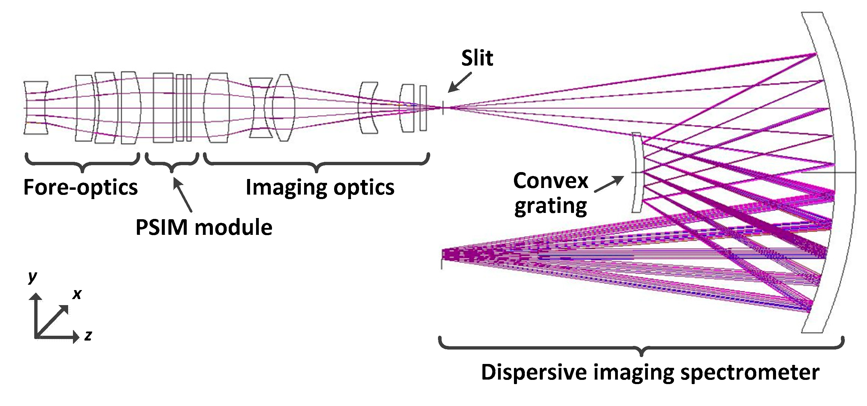
To verify the feasibility and advantages of the presented method, simulations experiment for the calibration of parameters in the polarization radiometric calibration model and reconstruction of Stokes parameters are performed. In the simulations, we use a fieldable CDISP designed for airborne remote sensing in advance, whose schematic layout is shown in Figure 2. It operates over 13,000–18,000 cm⁻¹, the FOV is 40° and the F-number is 4. R₁ and R₂ are made of quartz, whose birefringence in the selected wave band can be referred to Ref. [21], and their thicknesses are 6mm and 2 mm, respectively. We analyze the polarization properties of each sub-modules through polarization ray tracing [22,23] and calculate the phase retardations of R₂ and R₁ at different field of view. These results are used as the input values of the simulations. We compare the calibration results of parameters in the polarization radiometric calibration model and reconstructed Stokes parameters with two methods, i.e., the presented method in this paper, and the traditional calibration method of spectropolarimeter. Both methods take into account the alignment errors of polarization module and the variation of the retardations at different field of view in the process of radiometric calibration. The only difference is that in the radiometric calibration, the presented method considers the influence of polarization properties of optical system and decouples it, while the traditional calibration method does not consider its influence.

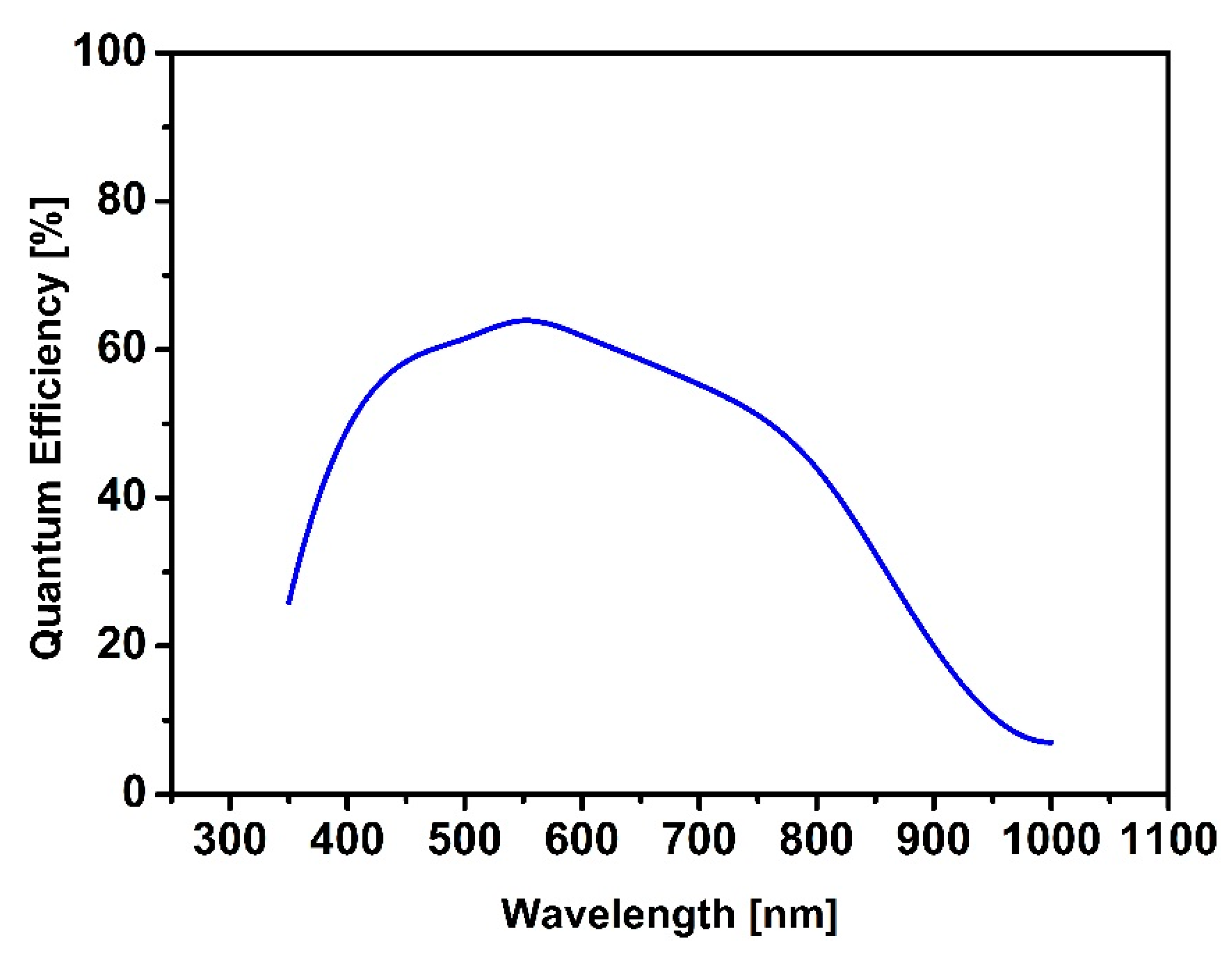
We first simulate the process of radiometric calibration of the fieldable CDISP. The detector uses SARNOFF’s CAM512 CCD as an example, whose area array is 512 × 512, the pixel size is $18\mu m\times 18\mu m,$ the frame frequency is 100 fps, and the quantum efficiency curve is shown in Figure 3. According to the imaging chain analysis of the radiance from optical system entrance pupil to detector, the DN recorded by detector can be obtained by simulation. Using the radiance of the optical system entrance pupil and the simulated DN of detector, the dark current response $C\left(\sigma ,\theta \right)$ and modulated radiometric calibration coefficient $A^{k^{\prime }}\left(\sigma ,\theta \right)$ can be obtained on the basis of the classical radiometric calibration principle.

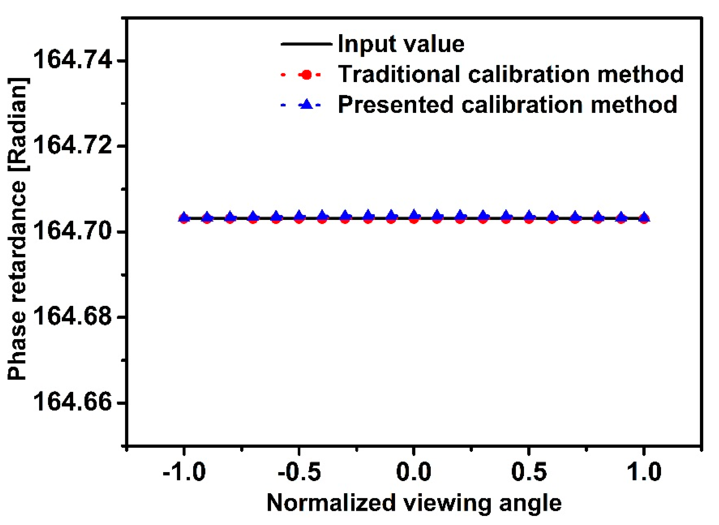
Next, we calibrate the alignment errors ${\epsilon }_1,$ ${\epsilon }_2$ and retardation ${\phi }_2\left(\sigma \right)$ of the PSIM module by using the self-correction method. The alignment errors of R₁ and R₂ are ${\epsilon }_1=-0.5°,$ ${\epsilon }_2=0.5°,$ respectively. Because the alignment errors are independent of wavenumber, we can use the averages of the calculated values in different wavenumbers as the final determination results, which are both −0.5029°and 0.5007° by the presented method and the traditional calibration method. The input values and calibration results of ${\phi }_2\left(\sigma \right)$ at different field of view is shown in Figure 4. The field of view is normalized and the wavenumber is 16,000 cm⁻¹. In order to facilitate quantitative analysis of the calibration results, we calculate ${\phi }_2\left(\sigma \right)$ from $\exp \left[i{\phi }_2\left(\sigma \right)\right]$ by using a phase unwrapping algorithm, though it is not needed in the calibration and reconstruction. The maximum residual error of ${\phi }_2\left(\sigma \right)$ is less than 1.0 × 10⁻³ rad. These calibration results indicate that the self-correction method is applicative for the fieldable CDISP. Since ${\epsilon }_1,$ ${\epsilon }_2$, and ${\phi }_2\left(\sigma \right)$ do not change with the field of view, it is feasible to calibrate them only by using the data at central FOV. The reference beam at central FOV is shined on the system along the optical axis at the center of the aperture, therefore, the effect of polarization properties on calibration results can be ignored. The validity of the self-correction method for alignment errors and retardation calibration has been demonstrated by experiment [17].

According to the calibration results of the alignment errors ${\epsilon }_1,$ ${\epsilon }_2$ and retardation ${\phi }_2\left(\sigma \right)$ of the PSIM module, we could decouple the radiometric calibration coefficient $A^k\left(\sigma ,\theta \right)$ and diattenuation of fore-optics $D_{fore}\left(\sigma ,\theta \right)$ from modulated radiometric calibration coefficient $A^{k^{\prime }}\left(\sigma ,\theta \right)$. 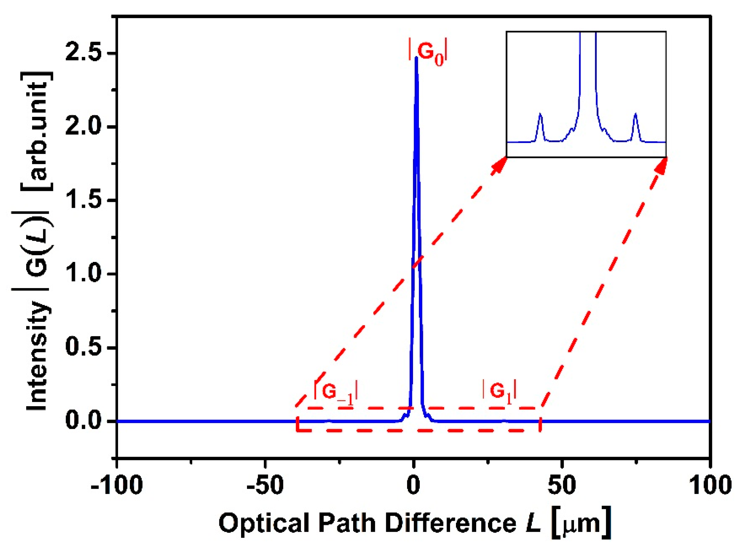Figure 5 gives the magnitude of the autocorrelation function of $A^{k^{\prime }}\left(\sigma ,\theta \right)$, which is at the edge FOV, the modulation channels of other FOV are consistent with this, only the amplitude is different. The figure only shows the values of channels 0 and 1, and the values of other channels are too small. Fortunately, only channels 0 and 1 are needed in the decoupling of $A^k\left(\sigma ,\theta \right)$ and $D_{fore}\left(\sigma ,\theta \right)$. 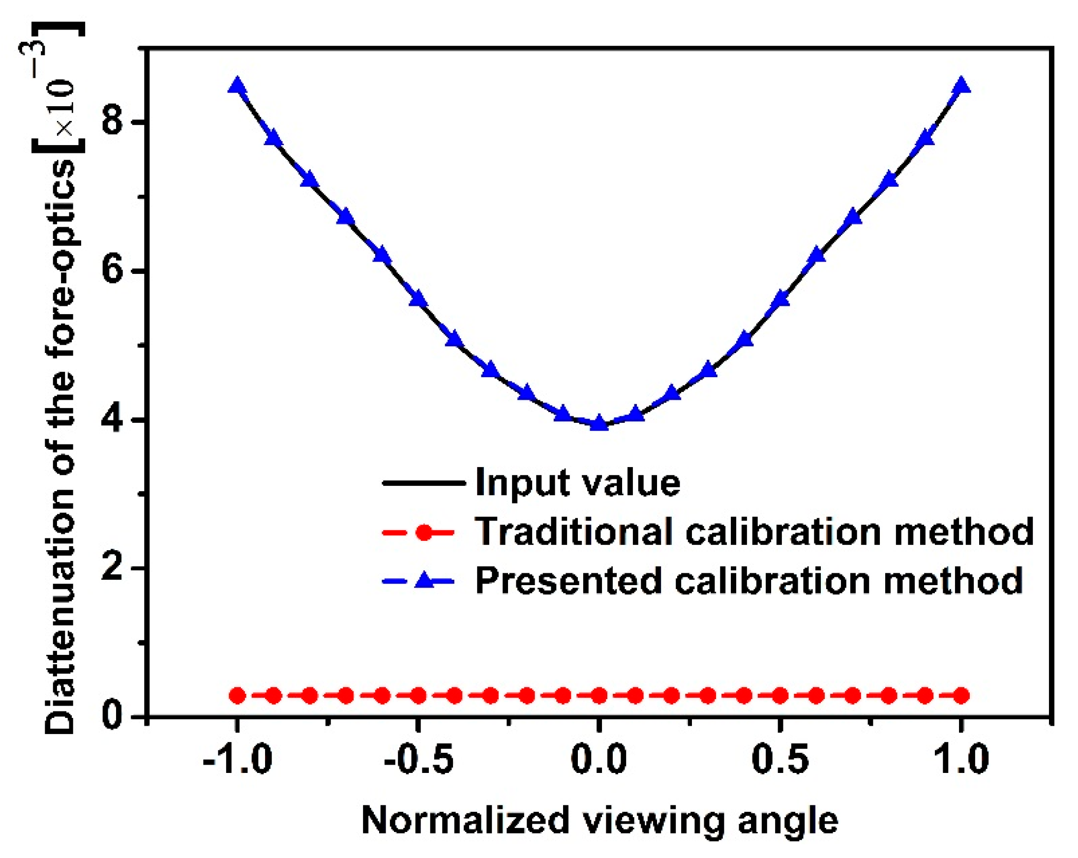The input values and calibration results of diattenuation of the fore-optics at different field of view are shown in Figure 6. And the maximum relative error of the calibration results of $D_{fore}\left(\sigma ,\theta \right)$ is less than 0.07% by using the presented method, while its maximum relative error is 63.57% by using the traditional calibration method. 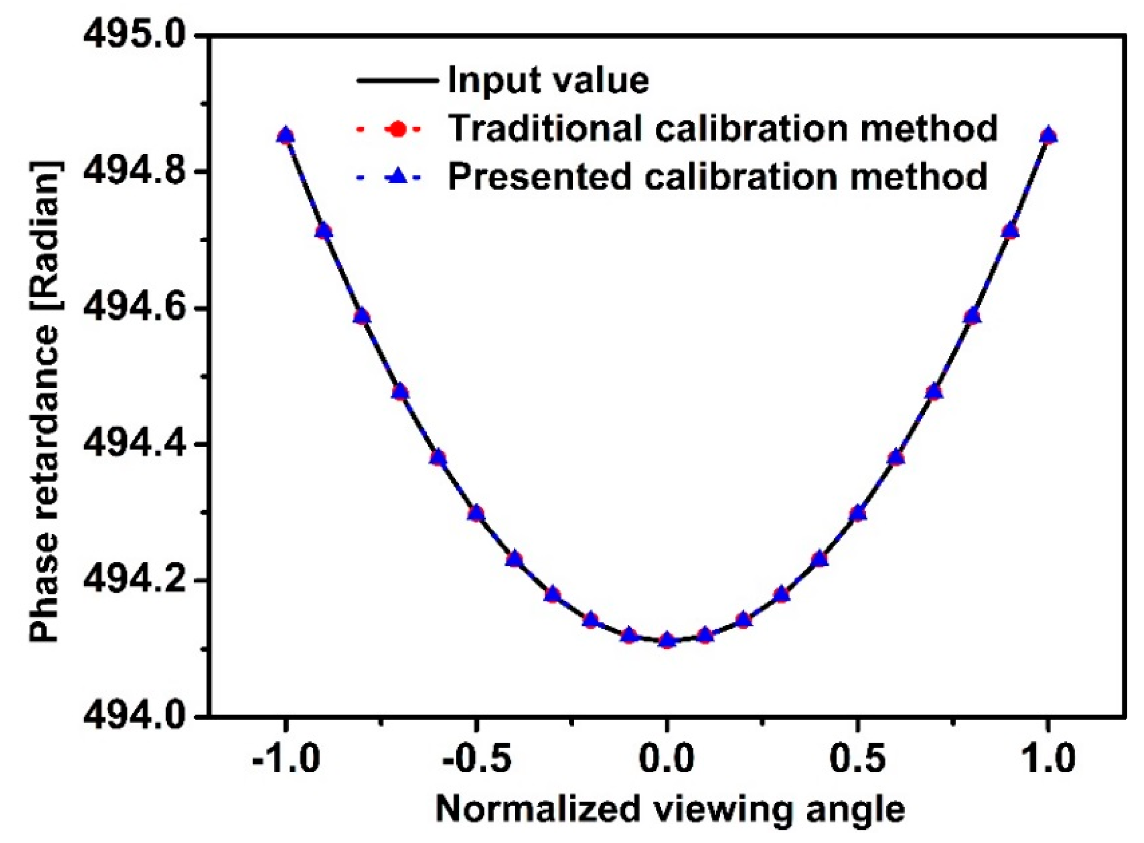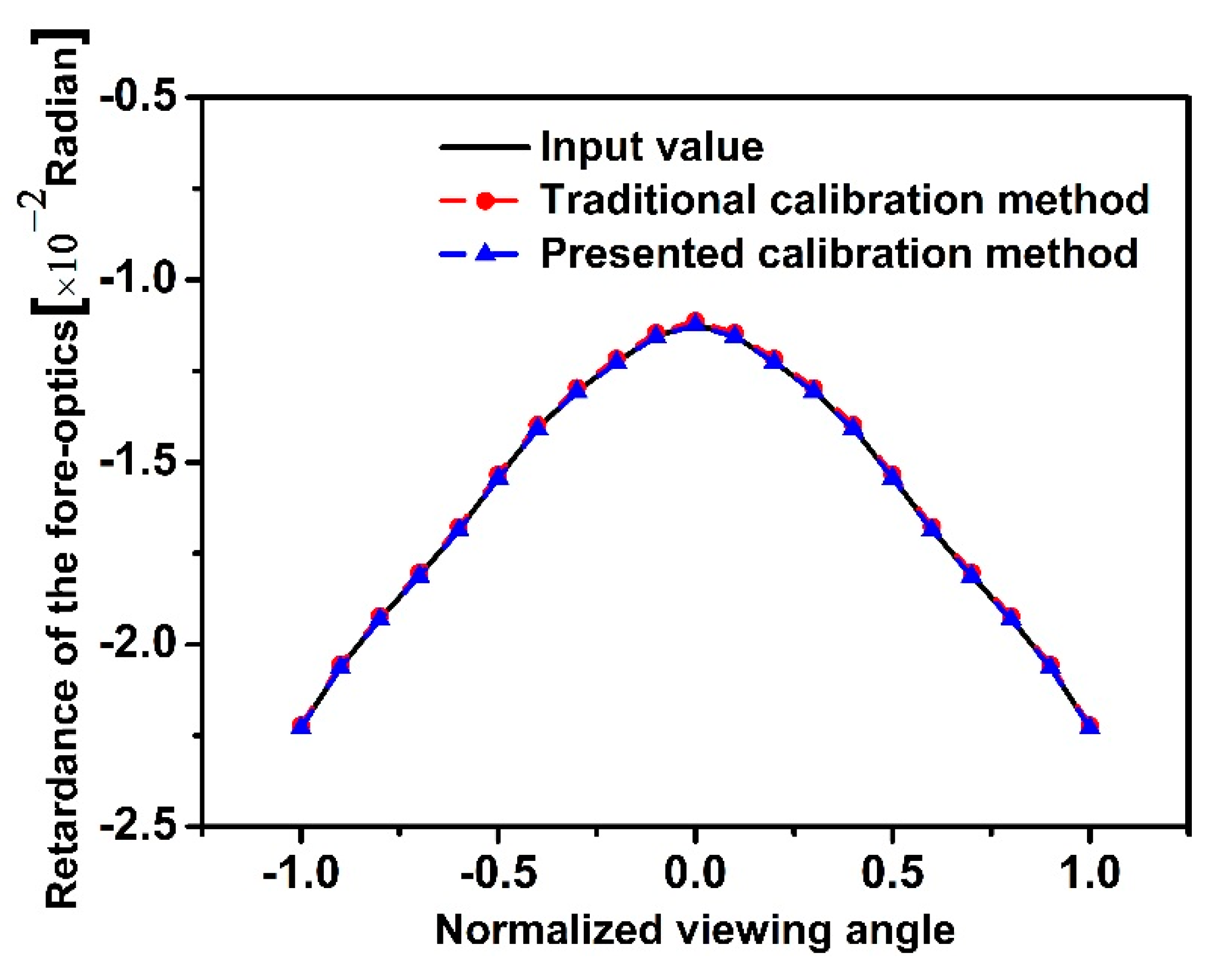Figure 7 and Figure 8 give the input values and calibration results of the retardation ${\phi }_1\left(\sigma ,\theta \right)$ and retardance of the fore-optics ${\delta }_{fore}\left(\sigma ,\theta \right)$ at different fields of view. In order to facilitate quantitative analysis of the calibration results, we calculate ${\phi }_1\left(\sigma ,\theta \right)$ from $\exp \left\{-i\left[{\phi }_1\left(\sigma ,\theta \right)+{\phi }_2\left(\sigma \right)\right]\right\}$ by using the calibration results ${\phi }_2\left(\sigma \right)$ and a phase unwrapping algorithm. The calibration results of ${\phi }_1\left(\sigma ,\theta \right)$ and ${\delta }_{fore}\left(\sigma ,\theta \right)$ of two methods are overlapped well with the input values, and the maximum residual errors are less than 1.0 × 10⁻⁴ rad. It can be seen that, compared with the traditional calibration method, the presented method can achieve more accurate calibration when calibrating diattenuation of the fore-optics. For the calibration of alignment errors, phase retardances in the PSIM module, and retardance of the fore-optics, the two methods can both get good calibration results.

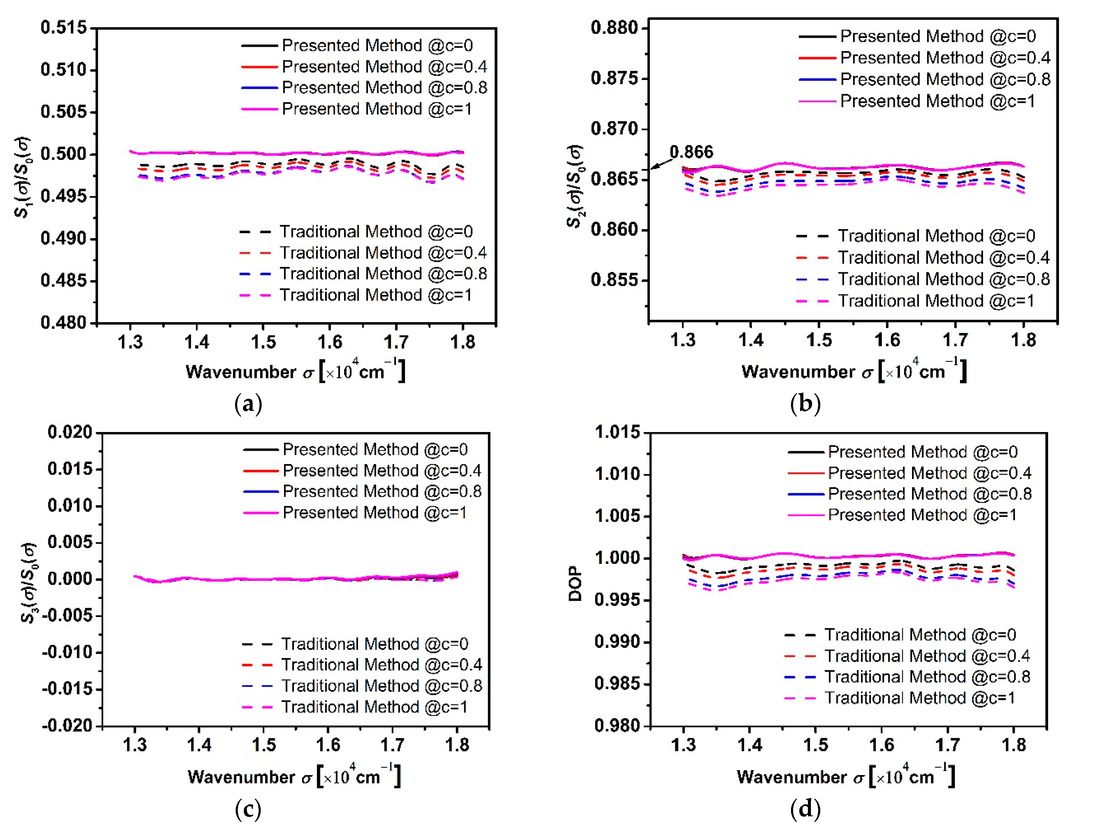
After calibrating the parameters in the polarization radiometric calibration model, we substitute these calibration results into Equations (12)–(15) to reconstruct the Stokes parameters of the target light. In the simulation, we employ a 30° linearly polarized beam as the target light, whose theoretical values of normalized Stokes vectors are S₁/S₀ = 0.5, S₂/S₀ = 0.866, and S₃/S₀ = 0, respectively. Figure 9a–c give the normalized Stokes vectors reconstructed by two methods, wherein the solid and broken line respectively represent the presented calibration method and the traditional calibration method, and the different colors represent reconstruction results at different field of view. Through contrastive analysis, the deviations of the Stokes parameters reconstruction results obtained by the traditional calibration method from the input values are large, and they are different with the change of field of view. While the reconstruction results obtained by the presented method are closer to the input values and overlapped well with different field of view. The reason is analyzed mainly because the radiometric calibration of the traditional calibration method does not take into account the influence of the polarization properties of optical system, and the spectral radiance obtained by the radiometric calibration deviates from that at the entrance pupil, which lead to the great inaccuracy of the reconstruction results of Stokes parameters. In order to further quantitatively analyze the measurement accuracy of the polarization information of the fieldable CDISP, we use the degree of polarization (DOP) [24], given by $DOP\left(\sigma \right)=\sqrt{S_1{}^2\left(\sigma \right)+S_2{}^2\left(\sigma \right)+S_3{}^2\left(\sigma \right)}/S_0\left(\sigma \right),$ to further analyze the reconstruction results, which are shown in Figure 9d.

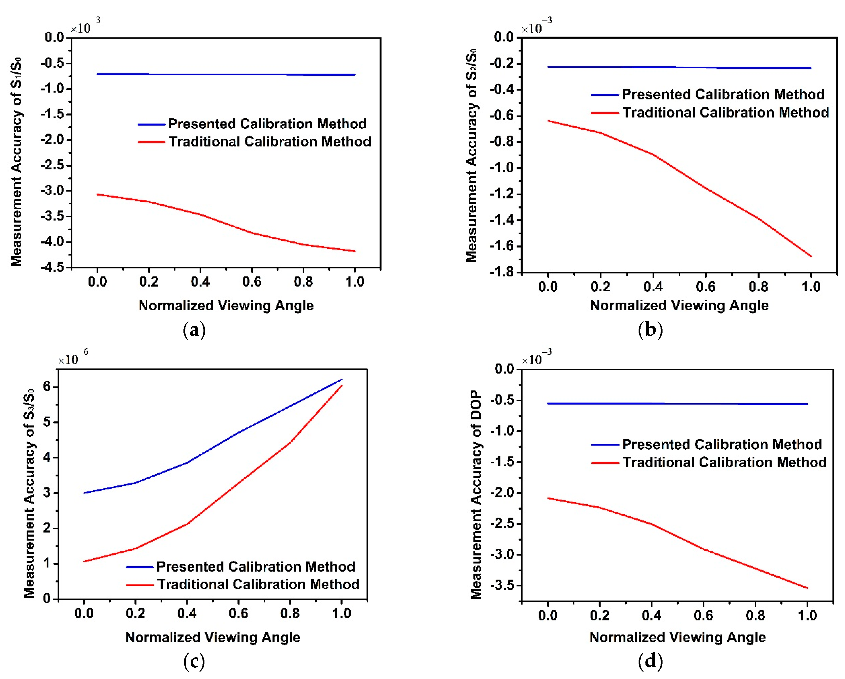
With these two calibration methods, the measurement accuracy of normalized Stokes vectors and DOP obtained from central to edge FOV are shown in Figure 10. It can be seen that the measurement accuracy of polarization information obtained by the traditional calibration method is decreased as the FOV increases. It is noteworthy that the measurement accuracy is about the same at different field of view by using the presented calibration method, and they are reduced by approximately an order of magnitude compared with the traditional calibration method. Though the measurement accuracy of S₃/S₀ by the presented method is less accurate than the traditional method, they are on an order of magnitude and are all very precise. The influence of the polarization properties of an optical system on the radiometric calibration of the fieldable CDISP is effectively compensated.

Since the CDISP studied in this paper is mainly used for airborne remote sensing, the circular polarization component of the target light is usually small enough to be ignored in practical applications, so we use the linearly polarized beam as the target light to verify the validity of the presented calibration method in simulation experiment.

5. Conclusions

The difficulty of the calibration for the fieldable CDISP lies in the decoupling of radiometric calibration coefficient and diattenuation of fore-optics. In this paper, we propose a polarization radiometric calibration model to decouple them. We first theoretically derive the calibration and compensation model considering the alignment errors of PSIM, the variation of retardations, and the polarization properties at different field of view of optical system. Before decoupling the radiometric calibration coefficient and the polarization properties, we perform classical radiometric calibration and self-correction calibration for the system. Finally, we use 0° and 45° linearly polarized beams to calibrate other parameters. By using the decoupled radiometric calibration coefficient and above-mentioned calibration results, we can accurately obtain the spectral radiance and reconstruct the polarization information of detected object. The validity and feasibility of the presented method have been confirmed by simulation experiments, and the reconstruction accuracy of the polarization information is improved compared with the traditional calibration method. The presented calibration method is significant for the quantitative application of the CDISP.

For the integral calibration process for the practical application of CDISP, the spectral calibration is not discussed in this paper. This is because the spectral calibration of CDISP is consistent with the calibration method of traditional dispersive imaging spectrometer, which can be completed in front of the polarization radiometric calibration.

References

1. Van Harten, G.; De Boer, J.; Rietjens, J.H.H.; Di Noia, A.; Snik, F.; Volten, H.; Smit, J.M.; Hasekamp, O.P.; Henzing, J.S.; Keller, C.U. Atmospheric aerosol characterization with a ground-based SPEX spectropolarimetric instrument. Atmos. Meas. Tech. 2014, 7, 4341–4351. [Google Scholar]
2. Noriyuki, N.; Frederic, A.; Ryohko, I.; Ryouhei, K.; Saku., T.; Amy, R.W.; Ken, K. Vacuum ultraviolet spectropolarimeter design for precise polarization measurements. Appl. Opt. 2015, 54, 2080–2084. [Google Scholar]
3. Stephen, H.J.; Frank, J.I.; Paul, L.K. Realization of quantitative-grade fieldable snapshot imaging spectropolarimeter. Opt. Express 2004, 12, 6559–6573. [Google Scholar]
4. Michael, W.K.; Mariano, E.L.; Julia, M.C.; Charles, F.L. Field deployable pushbroom hyperspectral imaging polarimeter. Opt. Eng. 2017, 56, 21435–21453. [Google Scholar]
5. Julia, C.; Michael, W.K.; Maryn, G.S.; Eustace, L.D. Compact Infrared Hyperspectral Imaging Polarimeter. Proc. SPIE 2010, 7695, 769509. [Google Scholar]
6. Chunmin, Z.; Haiying, W.; Jie, L. Fourier transform hyperspectral imaging polarimeter for remote sensing. Opt. Eng. 2011, 50, 066201. [Google Scholar]
7. Dubreuil, M.; Rivet, S.; Le Jeune, B.; Dupont, L. Time-resolved switching analysis of a ferroelectric liquid crystal by snapshot Mueller matrix polarimetry. Opt. Lett. 2017, 35, 103107. [Google Scholar]
8. Hiroshi, O.; Masayuki, H.; Hitoshi, N.; Atsushi, T.; Kazuhiko, O. Spectroscopic polarimetry using channeled spectroscopic polarization state generator (CSPSG). Opt. Express 2007, 15, 3093–3109. [Google Scholar]
9. Kazuhiko, O.; Takayuki, K. Spectroscopic polarimetry with a channeled spectrum. Opt. Lett. 1999, 24, 1475–1477. [Google Scholar]
10. Frank, J.I.; Stephen, H.J.; Herman, E.S.; Paul, K. Polarimetric-spectral intensity modulation (P-SIM): Enabling simultaneous hyperspectral and polarimetric imaging. Proc. SPIE 1999, 3698, 474–481. [Google Scholar]
11. Stephen, H.J.; Frank, J.I.; Chris, H.; Brian, C.; Anthony, C.; John, H.; David, H.; Yongxiang, H.; David, F. Preliminary airborne measurement results from the Hyperspectral Polarimeter for Aerosol Retrievals (HySPAR). NASA Earth Sci. Technol. Conf. Proc. 2006, 1, 1–6. [Google Scholar]
12. Tyo, J.S.; Turner, T.S. Variable-retardance, Fourier-transform imaging spectropolarimeters for visible spectrum remote sensing. Appl. Opt. 2001, 40, 1450–1458. [Google Scholar] [PubMed] [Green Version]
13. Riley, W.A.; Corrie, V.; Eustace, L.D.; Robert, S.; Robert., W.M. Snapshot imaging spectropolarimetry in the visible and infrared. Proc. SPIE 2008, 6972, 69720D. [Google Scholar]
14. Nathan, H.; Eustace, L.D.; David, T.S. Visible snapshot imaging spectro-polarimeter. Proc. SPIE 2005, 5888, 588810. [Google Scholar]
15. Chunmin, Z.; Qiwei, L.; Tingyu, Y.; Tingkui, M.; Yutong, W. High throughput static channeled interference imaging spectropolarimeter based on a Savart polariscope. Opt. Express 2016, 24, 23314–23332. [Google Scholar]
16. Bin, Y.; Junqiang, Z.; Changxiang, Y.; Xueping, J. Methods of polarimetric calibration and reconstruction for a fieldable channeled dispersive imaging spectropolarimeter. Appl. Opt. 2017, 56, 8477–8491. [Google Scholar]
17. Wenhe, X.; Xueping, J.; Changxiang, Y.; Bin, Y.; Junqiang, Z. Self-correction of alignment errors and retardations for a channeled spectropolarimeter. Appl. Opt. 2018, 57, 7857–7864. [Google Scholar]
18. Russell, A.C. Mueller matrices. In Handbook of Optics, 3rd ed.; Bass, M., Ed.; McGraw-Hill: New York, NY, USA, 1995; Volume 1, pp. 14.1–14.44. [Google Scholar]
19. Liangliang, Z. Correction of non-uniformity response for multiple output TDI CCD imaging system. Infrared Laser Eng. 2014, 43, 145–150. [Google Scholar]
20. Mingxin, L.; Xin, Z.; Tao, L.; Guangwei, S.; Lingjie, W.; Yi, L. On-Orbit Polarization Calibration for Multichannel Polarimetric Camera. Appl. Sci. 2019, 9, 1424. [Google Scholar]
21. Russell, A.C. Polarizer. In Handbook of Optics, 3rd ed.; Bass, M., Ed.; McGraw-Hill: New York, NY, USA, 1995; Volume 1, pp. 13.1–13.58. [Google Scholar]
22. Russell, A.C. Polarization ray tracing. Proc. SPIE 1987, 766, 61–68. [Google Scholar]
23. Russell, A.C. Polarization analysis of optical systems. Opt. Eng. 1989, 28, 280290. [Google Scholar]
24. Peralta, R.J.; Nardell, C.; Cairns, B.; Russell, E.E.; Travis, L.D.; Mishchenko, M.I.; Hooker, R.J. Aerosol polarimetry sensor for the Glory Mission. Proc. SPIE 2007, 6786, 67865L. [Google Scholar]
Figure 1. Optical schematic of the fieldable CDISP.
Applsci 10 08295 g001
Figure 2. Schematic layout of the fieldable CDISP.
Applsci 10 08295 g002
Figure 3. Quantum Efficiency curve of the detector.
Applsci 10 08295 g003
Figure 4. Input values and calibration results of φ 2 ( σ )
Applsci 10 08295 g004
Figure 5. Magnitude of the autocorrelation function of A k ( σ , 1 )
Applsci 10 08295 g005
Figure 6. Input values and calibration results of the diattenuation of the fore-optics.
Applsci 10 08295 g006
Figure 7. Input values and calibration results of φ 1 ( σ , θ )
Applsci 10 08295 g007
Figure 8. Input values and calibration results of the ratardance of the fore-optics.
Applsci 10 08295 g008
Figure 9. Reconstructed results of normalized Stokes parameters and DOP, wherein the solid and broken line respectively represent the presented calibration method and the traditional calibration method, and the different colors represent reconstruction results at different field of view. (a) S1/S0; (b) S2/S0; (c) S3/S0; and (d) DOP.
Applsci 10 08295 g009
Figure 10. Measurement accuracy of normalized Stokes vectors and DOP, (a) S1/S0; (b) S2/S0; (c) S3/S0; and (d) DOP. Wherein the blue and red lines respectively represent the presented calibration method and the traditional calibration method.
Applsci 10 08295 g010
Publisher’s Note: MDPI stays neutral with regard to jurisdictional claims in published maps and institutional affiliations.