Article

Modular System-Level Modeling Method for the Susceptibility Prediction of Balise Information Transmission System

1
Electromagnetic Compatibility Research Institution, School of Electronic and Information Engineering, Beijing Jiaotong University, Beijing 100044, China
2
Beijing Engineering Research Center of EMC and GNSS Technology for Rail Transportation, Beijing 100044, China
*
Authors to whom correspondence should be addressed.
Appl. Sci. 2020, 10(21), 7944; https://doi.org/10.3390/app10217944
Submission received: 20 August 2020 / Revised: 28 October 2020 / Accepted: 5 November 2020 / Published: 9 November 2020
(This article belongs to the Special Issue Recent Advances in Sustainable Process Design and Optimization)

Abstract

:
For high-speed train, balise transmission module (BTM) system is easily interfered with by other equipment of the train. This could cause the train to malfunction. Studying the electromagnetic susceptibility (EMS) of the BTM is very important for the performance and efficiency of the train. In this paper, a modular, system-level modeling method is proposed to predict the EMS of BTM systems. Based on object-oriented technology and a modular method, the BTM system is disassembled into several modules according to the electromagnetic characteristics of the whole system rather than the physical structure. All the modules are mutually independent, and the total EMS could be evaluated by the output of them. The modules of three key elements of electromagnetic compatibility (EMC), i.e., sources, coupling paths, and sensitive equipment, are established by the theoretical method, full-wave simulation method, and black-box test method, respectively, and put into different layers. According to the functions of the BTM system, the EMS of BTM is given by analyzing the interrelation of input and output of modules. Results of the proposed model were verified by measurement.

1. Introduction

The balise transmission module (BTM) system is a subsystem of the train operation control system for high-speed trains. It is responsible for detecting the presence of a balise and obtaining the location information of the train. As a positioning sensor, BTM system is comprised of BTM, on-board antenna, balise and wayside equipment, as shown in Figure 1. The on-board antenna at the bottom of the train receives the RF signal from balise to get the location information. Due to the complex and harsh train bottom electromagnetic environment, the RF signal from balise is interfered with easily and the BTM system will not work properly. This could lead to serious consequences, such as location information decoding error or stopping the train [1]. Thus, it is of great significance to study the EMS of BTM for ensuring the normal work of BTM system under interference condition and the efficient operation of the train.
There are several researches on the electromagnetic interference (EMI) of BTM systems. Most of them focus on analyzing the EMI coupling process in different balise allocated positions and different operating modes of the system [2,3,4,5,6]. The BTM system EMC issues are mentioned in European SUBSET 036 and European SUBSET 085, but not described in detail [7,8]. In European SUBSET 116, EMC test methods are defined for analyzing the BTM system with disturbance [9], but it is still in draft. There are a few researches on the EMS of BTM system [10,11] presented the test method in the laboratory. It is recommended for EMS research of manufactured equipment, but not suitable in the design phase of BTM system. A more detailed and practical method for EMS prediction and system analysis should be investigated.
From function perspective, a high-speed train consists of several subsystems: train operation control, traction power supply, brake control and network communication systems. BTM system is a subsystem in the train operation control system. From EMC perspective, the EMI of BTM system could be from different coupling paths and other subsystems in the train, i.e., it is a system-level problem which could not be solved only in device-level within the subsystem. A device-level issue means an issue related to certain devices. For example, the influence from traction converter of the traction power supply system to the balise is a device-level issue. When the disturbance to a BTM system occurs and it is not clear which devices or subsystems are the sources and which devices are the victims, the analysis on the interaction between all the devices of BTM system and all the subsystem of the train is a system-level issue. In practice, almost all the EMC problems are system-level issues. However, most of EMS prediction methods solve the device-level EMS issue [12,13,14]. Even if electromagnetic topology method is regarded as a typical approach for system-level EMC analysis [15,16,17] the complicated huge system cannot be settled due to the increasing complexity of the topology structure with a rapid increase of nodes and harassment transmission paths. The concept of hierarchical method is proposed to simplify the system-level EMC analysis problem [18]. It is a “flow down” method, which means it can solve the EMI problem from device-level to system-level, but ignores the interaction between device and system. It is not suitable for predicting the EMI problem of the BTM system in practical engineering applications which is in the unstable electromagnetic environment. The working environment of BTM system would be affected by the changes of other subsystems in the train, e.g., the pantograph off-line disturbance, the emission from rail return current and other disturbances from the traction power supply system. In addition, the EMS of the BTM system should also consider the function of the system itself.
Modular system-level modeling and prediction method is proposed in this paper based on the object-oriented analysis method (OOAM) [19]. For this approach, the system is rebuilt based on electromagnetic characteristics. The devices with the same electromagnetic characteristics are extracted as one object. Moreover, the objects with the same function are utilized to classify and integrate in a module model according to the concept of object-oriented technology and the modular method [20]. Based on the concept of a hierarchical structure, three layers are built according to EMC key elements, the EMI source, coupling path and sensitive device [21]. The module models are classified by these three layers and a complete system-level model is built. All these modules are interrelated with their input and output state. The interaction of devices in the whole system is realized through the interaction between modules. It is effective to simplify the system-level EMC analysis because modules are mutually independent and just affiliated with the attributes of objects. According to the needs of practical engineering problems, any module could be selected or connected to simulate and analyze the device-level, subsystem-level, and system-level EMC problem. Moreover, for this model, the functions of device and system are defined as the attributes. The interrelation of functions and prediction could be got easily.
This paper is organized into five sections. In Section 2, the modular system-level prediction modeling procedure is presented. Module analysis for on-board device of BTM system is given in Section 3. In Section 4, the comparisons between the proposed modeling methodology and measurement are shown. Conclusions are given in Section 5.

2. Modular System-Level Modeling Approach

The BTM system has three normal functions. With some generality, it would cause the harmful consequences when the BTM system is interfered with [9], as listed in Table 1.
BTM system should take function F1 first before the system starts working. This function is enabled only when the BTM system starts to work. A test data package will transmit by radio-frequency energy transmitting antenna through route 1 and received by on-board antenna, as shown in Figure 2a. Secondly, after passing the self-test, the BTM system enforces function F2 to find the balise. This function is enabled all the time during travel. When the on-board antenna moved into the Main Lobe Zone of the balise shown in Figure 2b, function F3 is waking up [7]. This function will enable the on-board antenna to start receiving 2FSK message from balise through route 2, the air gap which is called interface A, as shown in Figure 2a, and help the BTM extract the location information from the message. During the above processes, a variety of disturbances could be coupled to on-board antenna and signal cable through different coupling path shown in Figure 2a at any time.

2.1. Modular System-Level Model

The modular system-level model is made up of mutually independent modules. Thus, to build the modular system-level model, the electromagnetic characteristics of the whole system should be considered.
According to researches and on-site experience, the disturbance source could be classified into three forms: conducted, induced, and radiated form which are mutually independent. Therefore, three source modules are built for BTM system: radiation disturbance, conducted disturbance and induction disturbance modules. The devices in the BTM system, which are sensitive to interference, are encapsulated as sensitive equipment module. The disturbances need paths to “go” into BTM system like ground loops, radiation and the cable crosstalk coupling [22]. Thus, radiation, conduction, and induction coupling modules could be built according to the coupling path. All the modules are linked by the input and output port of them.
Each module is the encapsulation of objects, which are the devices or components with the same electromagnetic characteristics. For example, the radiation coupling modular model contains antenna, aperture, and wires object models. One object may have lots of properties. Table 2 lists a few object properties, which is utilized to build BTM EMS prediction model. The character of modules will be changed only by changing these electromagnetic properties of the object model.
Then, all the modules are put into three layers and the whole modular system-level model is completed. The three layers are divided based on three elements of EMC, i.e., electromagnetic disturbance source, EMI coupling, and sensitive equipment layers, as shown in Figure 3.

2.2. Prediction Procedure

To analyze EMS for BTM system, the only thing should be considered is the input and output of the modules in this prediction model. The prediction procedure for EMS prediction is shown in Figure 4.
S1, S2, S3 represent the radiated disturbance, inducted disturbance, and conducted disturbance respectively. The value of disturbance S1, S2, S3 depend on the train operation state or other subsystem working state. C1, C2, C3 are the coupling function of radiation, induction, and conduction respectively. The gate function set is determined according to the relationship between the modules in different layers. Here, the gate function set consists of two types: Fs and Fc. Fs indicates the connection between the electromagnetic disturbance source layer and EMI coupling layer, while Fc is used to establish the connection between EMI coupling layer and sensitive equipment layer.
F s = { F s 1 , F s 2 , F s 3 } F c = { F c 1 , F c 2 , F c 3 } ,
Due to the flexibility of object-oriented module modeling method, the module could be used as the requirement of system-level analysis. Every element of gate function set F consists of 0 or 1. “0” represents there is no connection between the two modules, and “1” is the opposite. For example, if induction disturbance module and inductive coupling module interact with each other, Fs2 = 1, otherwise Fs2 = 0.
Sr1 is the disturbance signal produced from S1 and went through the on-board antenna by radiation coupling. Meanwhile, Sr2 is the disturbance signal produced from S2, effected by Fs2 and goes through the antenna cable by inductive coupling like cables crosstalk or antenna by inductive coupling like near field coupling. And disturbance signal Sr3 is produced from S3 and goes through the cables in the BTM system by conductive coupling. All these three disturbance signals Sr1, Sr2, and Sr3 would act on the input port of BTM at the same time. Sn at the input port of BTM is composed of Sr1, Sr2 and Sr3. EMS prediction of BTM system is to analyze what kind of disturbances will lead to inevitable performance degradation for the system. T is defined as the critical condition for sensitive equipment normal operation. That means T is the basic requirements of routine operation for sensitive equipment. The critical condition T relies on the three functions of the system mentioned at the beginning of Section 2. “Sn = T” stands for the system could work well with the disturbance Sn. Increase the voltage of S1, S2 or S3, until the disturbance Sn just make the system could not work properly. For easy manipulation on-site, voltage is chosen to assess the value of the disturbance Sn in EMS prediction. Thus, the disturbance voltage VN is considered as the sensitivity level of BTM system. And VN could be expressed as the summary of Vr1, Vr2 and Vr3 the voltages of Sr1 Sr2 and Sr3.
V N = V r 1 + V r 2 + V r 3 ,
where,
V r 1 = V 1 F s 1 C 1 F c 1 V r 2 = V 2 F s 2 C 2 F c 2 V r 3 = V 2 F s 3 C 3 F c 3 ,
where V1, V2, and V3 are the voltages of disturbance signal S1, S2, and S3 respectively. If the sensitivity level of BTM system is confirmed, the value of VN is a determined value.
According to this prediction procedure, the sensitivity level of BTM system is a key factor and needed to be calculated for different BTM system functions.

2.3. Model for BTM Susceptibility Prediction

To find out the main disturbance coupling path for BTM system, the comparative experiment is taken during the train passes the neutral zone. The setup of the first experiment is shown in the Figure 5a: the disturbance received by the on-board antenna is measured directly by a spectrum analyzer. Another experiment configuration is shown in the Figure 5b: An impedance of 50 Ω is used to take the place of BTM antenna, then the disturbance is measured by the spectrum analyzer in zero span mode.
The comparison result is shown in Figure 6. The maximum disturbance voltage is 77 dBμV when the antenna connection, shown in Figure 6a. The maximum disturbance voltage is 47 dBμV when the antenna is disconnected and is replaced by 50 Ω, shown in Figure 6b. Thus, the main disturbance coupling path for BTM system is antenna coupling.
For railway system, the two most serious disturbances are generated from traction power system. One is pantograph off-line disturbance when the train passes through phase separation zones, and the other one is traction return current. In order to confirm the main disturbance source, a further field tests have been done. An “antenna connection” setup is taken when the train is in a normal operational situation. In this situation, traction return current is considered to be the main disturbance source. And the disturbance received by the on-board antenna is shown in Figure 7. The disturbance levels are almost the same with the result in Figure 6a which is obtained with pantograph off-line disturbance. Thus, the main disturbance does not come from the pantograph off-line disturbance, but induces from traction return current flowing on the steel rails and some other disturbance from traction power system. Moreover, according to the loop physical structure and operation frequency of BTM antenna, the main disturbance is in the form of magnetic field [23].
Based on the analysis above, the influence of radiation disturbance and conductive disturbance could be ignored. Thus, it is assumed that the voltages of Sr1 and Sr3 in Figure 4 equal to zero. The modules for radiation and conducted disturbance could be ignored. For modular system-level modeling method in the paper, the module could be utilized alone according to requirements for practical problems. Thus, the BTM EMS prediction model could be simplified as induction disturbance, induction coupling, and sensitive equipment modules, as shown in Figure 8.
Thus, according to the method the Fs2, Fc2 equal to 1 and other elements of transfer function equal to 0., the disturbance voltage VN could be obtained as Equation (4).
V N = V r 2 = V 2 C 2 ,

3. Modular Modeling for BTM System

The disturbance voltage VN at the input port of BTM is defined as the sensitivity of BTM system. From Equation (4), disturbance voltage V2 of induction disturbance module, coupling function C2 of inductive coupling module and the critical condition T are important to get VN. Thus, the key point of the system-level modeling approach is modular modeling, which could be dealt with by different methods. To establish the model in Figure 8, theory method, full-wave simulation method, and black-box test method are utilized for the induction disturbance source module, induction coupling module, and sensitive equipment module, respectively.

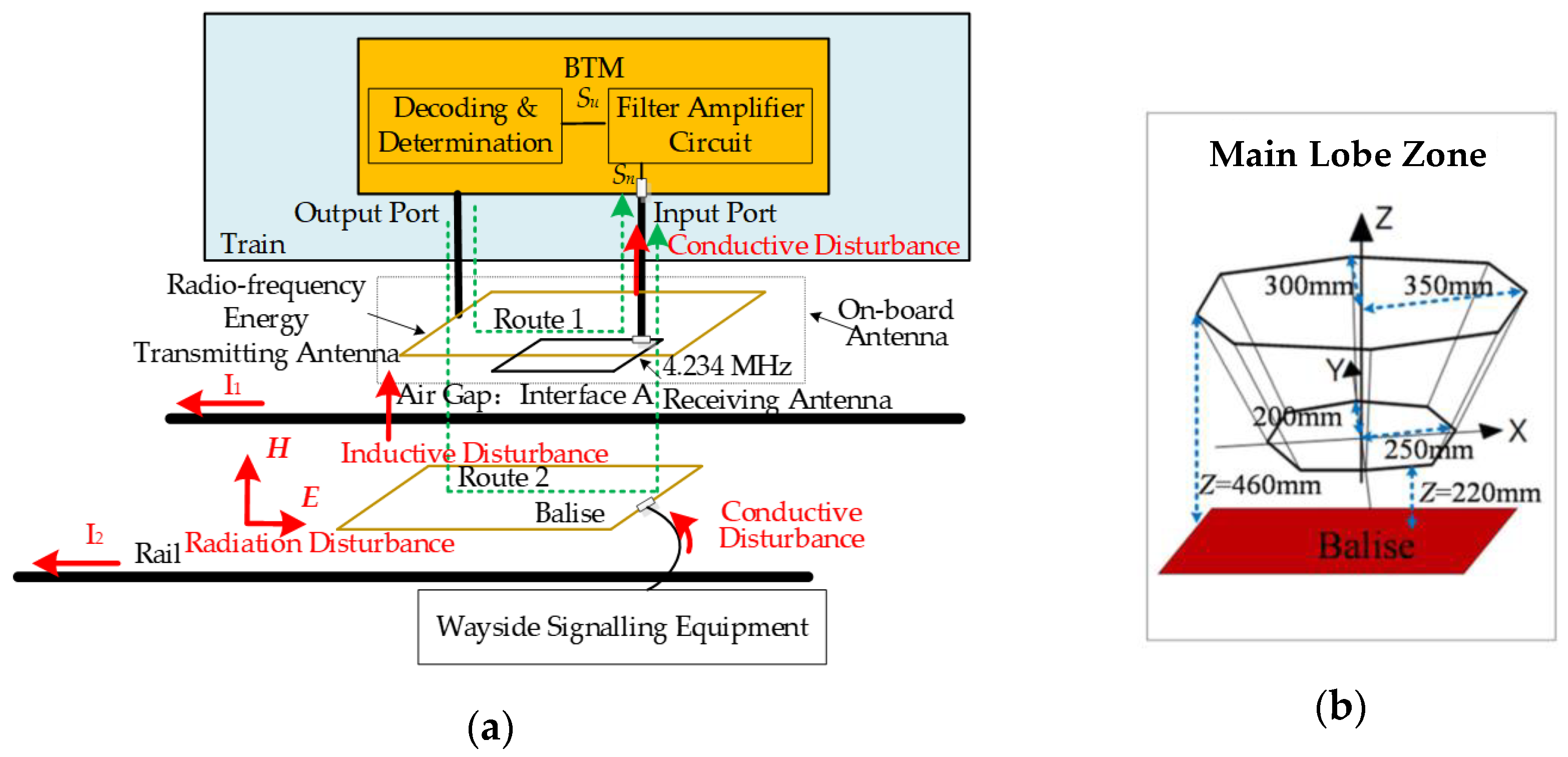
3.1. Modeling for Induction Disturbance Source Module

As a loop antenna, the on-board antenna gets the location information and other useful messages transmitted from balise by receiving the magnetic field signal. Meanwhile, the disturbance would be coupled to the on-board antenna too. To quantify the magnetic field disturbance, the induction disturbance source module is established by using a rectangular loop antenna with a current source I, as shown in Figure 9.
The side length of the rectangular loop antenna are a and b respectively. When the rectangular loop antenna is electrically small, the magnetic field intensity at the field point P (x, y, z) could be calculated by Biot–Savart law [24],
B = μ 0 I 4 π l o o p d l × 1 R .
According to Equation (5), the magnetic field disturbance is related to the size of the rectangular loop antenna, the distance R and the disturbance current I. Thus, when the position and the size of every device is fixed, the level of magnetic field disturbance is determined by current I. In the case of the electromagnetic environment on-site, these disturbances may be generated by the following sources which are laid close to the on-board antenna: current harmonics from the traction system, current from the rails and cables [23]. These disturbance currents could be pure sinusoidal continuous wave, transient, damped oscillation typology [9]. Using Fourier series, all of this disturbance could be described as a superposition of sinusoidal waves with different frequencies. Thus, to simplify the modeling process, pure sinusoidal continuous wave disturbance shall be applicable.
The voltage of induction disturbance S2 could be obtained as [25]
V 2 = I R s ,
where Rs is the port impedance of the rectangular loop antenna.

3.2. Modeling for Inductive Coupling Module

Depending on the working principle of on-board antenna, the inductive disturbance coupling module is established in Ansys HFSS and the S-parameters are solved by using the finite element method (FEM), as shown in Figure 10.
The size of EMI radiation antenna and the voltage of the induction disturbance S2 are considered as the output of induction disturbance source module. They perform as the input of the inductive coupling module. The size of the rectangular loop antenna is 240 × 430 mm. In addition, the size of the on-board antenna is 240 × 265 mm. Port 1 on the on-board antenna is the antenna receiving port, while the Port 2 on the EMI radiation antenna is disturbance transmitting port. The vertical distance of the two antennas is 460 mm based on the height from on-board antenna to the rail.
Set the center of the EMI radiation antenna to be at the ordinate origin. Train running orientation is the positive direction along Y-axis. The S-parameters of antennas shown in Figure 11a is the S12 as different horizontal distances between two antennas’ centers. The value of S12 keeps stable within the scope of ±0.2 m. Thus, S-parameter of the antenna system is used when on-board antenna is located right above the EMI radiation antenna.
The output power Ps from Port 2 and the input power Pr at Port 1 satisfy [26],
P r = P s | S 12 | 2 ,
To ensure the signal transmission performance, Rs and RBTM are set to 50 Ω. V2_eff and Vr2_eff are the effective values of V2 and Vr2. Thus, Ps and Pr are expressed as
P s = V 2 _ eff 2 R s ,
P r = V r 2 _ eff 2 R BTM ,
Thus, the port voltage Vr2 of on-board antenna is,
V r 2 = V 2 S 12 R BTM R s ,
The RBTM and Rs are the impedances of Port 1 and Port 2 respectively.
According to Equation (2), VN=Vr2, the inductive coupling function C2 is expressed as,
C 2 = S 12 R BTM R s ,

3.3. Modeling of Sensitive Equipment Module

For getting the critical condition T for sensitive equipment, the sensitive equipment module is modeled in two parts, as shown in Figure 2 with the filter amplifier circuit and the part for decoding and determination.
Ignoring cable loss, Sr is the input signal transmitting into the sensitive equipment module. It could be divided into two parts, useful signal S0 and disturbance signal Sn. Since the modulation of BTM system signal is 2FSK, the signal Sr received by BTM could express as [27],
S r ( t ) = S 0 ( t ) + S n ( t ) ,
where,
S 0 ( t ) t [ 0 , N T b ] = U pp k = 0 N [ Rect ( t k T b T b ) cos { 2 π [ ( f c + Δ f c ) + ( 2 b k 1 ) ( f m + Δ f m ) ] t + ϕ ( k T b ) } ] ,
where fc is the carrier frequency, fm is frequency offset, while Δfc and Δfm are the instability of carrier frequency and frequency offset, respectively. k is the length of data. Tb is the cycle of the baseband data signal and bk is the bit value. The useful signal S0(f) in the frequency domain is shown in Figure 12.
Su is the output signal from filter amplifier circuit [28],
S u ( f ) = S 0 ( f ) h + S n ( f ) h ,
where h is the transfer function of the filter amplifier circuit. It could be expressed as the magnitude-frequency characteristic of the filter amplifier circuit. The disturbance signal Sn going into the sensitive equipment could be quantified by measurement.
To get h, black-box testing method is used [29]. The setup of the test is shown in Figure 13.
As shown in Figure 14, the filter amplifier is a band pass filter working at the BTM band, and the amplifier factor is about 10 dB at 4.232 MHz. The BTM operating frequency range is defined as 3–6 MHz for this type of BTM system.
The information will be transferred to the Automatic Train Protection (ATP) system after decoding. The bit error rate could be obtained from formulations (12), (13), and (14) when the instability of carrier frequency and frequency offset is equal to zero [27].
p e = 1 2 e r f c ( E b 2 E N ) ,
where the Eb is the energy of the useful signal S0h. EN is the energy of the disturbance signal Snh [24].
E b = T ( S 0 h ) 2 R BTM d t E N = T ( S n h ) 2 R BTM d t ,
where RBTM is the input impedance of BTM.
For getting the critical condition T, the function of BTM system listed in Table 1 should be considered. Function F2 is simple comparing to the other two functions: F1 and F3, due to it does not involve signal analysis. Thus, the EMS for BTM system should be predicted in two ways for different functions.

3.3.1. T for BTM System with F2

In function F2, a balise shall be detected when the voltage of Su at the output port of the filter amplifier circuit segment of BTM is higher than Vth during a minimum time. If the on-board antenna is not at the contact zone, and the voltage of Su is larger than Vth, the BTM will erroneously report the existence of a balise. Thus, Vth is defined as the critical condition T in this function. Moreover, it is a known value for a certain BTM system.

3.3.2. T for BTM System with F1 or F3

The relationship between Signal Noise Ratio (SNR) and Bit Error Rate (BER) of BTM signal Su could be calculated by Equation (15). According to European standard SUBSET 036, the BER of BTM system should be below 10−6 when BTM system carries out F1 [7] and F3 function. Thus, the SNR of output signal Su should be larger than 13.5 dB according to BER of BTM system of Figure 15. That means, in function F1 and F3, the BTM should receive correct data when the SNR of Su is larger than 13.5 dB. And if the SNR of Su is lower than 13.5 dB, the BTM will fail to start or report erroneously localization of a balise even balise missing. Thus, the critical condition T could be set at SNR = 13.5 dB.
Significantly, the useful signal levels are different in these two functions, as shown in Figure 16, thus the sensitive disturbance levels should be calculated separately.
For a certain type of BTM system, the maximum electrical level of the test data received by BTM is 57.76 dBμV at 4.512 MHz and 56.43 dBμV at 3.95 MHz during “on-line transmission self-test” processing, shown in Figure 16a. It is the useful signal level in the self-test function. For “Data Reception Function”, the maximum signal level received by BTM is 77.76 dBμV, shown in Figure 16b.
To validate sensitive equipment module, field tests are carried out, shown in Figure 17. The differential-mode disturbance at the input of BTM is tested by the spectrum analyzer when the train stops and runs. For this train, the exhaust system locates near the on-board antenna of BTM. It may produce disturbance. In the test, when the train is running normally, BTM system could normally operate. If the train is going to run and the exhaust system power on initially, BTM system cannot start and the train cannot run either. However, if shutting down the exhaust system and making the BTM system start first, the train could start to work successfully. The disturbance at the input of BTM is shown in Figure 18. When the exhaust system works, the disturbance level is 58.59 dBμV at 3.95 MHz and 47.19 dBμV at 4.512 MHz. If the exhaust system is powered off, the disturbance level is around 40 dBμV at both 3.95 MHz and 4.512 MHz for this field test.
Based on the BTM signal level in Figure 16 and the disturbance level in Figure 18, the phenomenon could be explained by the modeling of sensitive equipment module.
When the exhaust system starts before the BTM system, the SNR is −2.16 dB at 3.95 MHz and 10.57 dB at 4.512 MHz. They all smaller than the critical condition T (SNR = 13.5 dB). Thus, the on-line transmission self-test fails and BTM system will not start. As a result, the train cannot operate either.
When BTM system starts first without exhaust system, the noise is low, and the smallest SNR is 16.43 dB at 3.95 MHz (the disturbance source level is 40 dBμV when exhaust system is powered off). Comparing to the critical condition T, the BTM system will pass on-line transmission self-test and start normally. During Data Reception function, the BTM useful signal is much higher than the noise. When the exhaust system started, the smallest SNR is 19.17 dB which is still larger than 13.5 dB. Therefore, the train could continue to operate normally.
Therefore, the model analysis could predict the EMS of BTM system well.

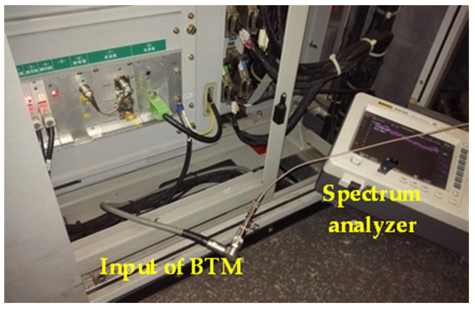
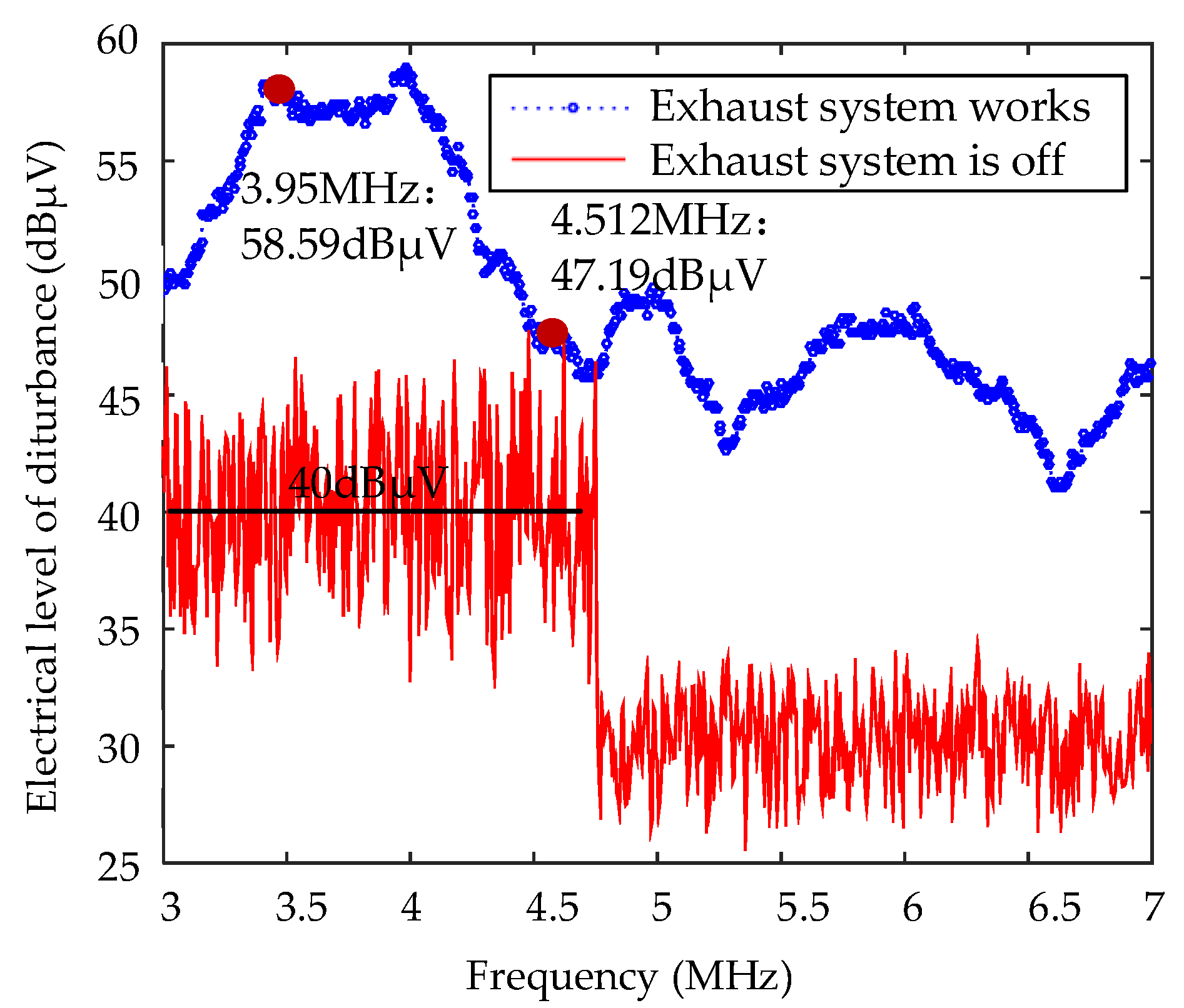
4. Analysis and Validation

Sensitivity of BTM system defined as the level of disturbance at the input port of BTM, which leads to the abnormal working status of BTM system.
To validate the modeling method, the sensitivity of BTM system is measured in a semi-anechoic chamber. Figure 19 shows the measurement set-up. The measurement was performed using two signal generators (RIGOL DG3121A signal generator and RIGOL DG1032Z signal generator) and a spectrum analyzer (ROHDE & SCHWARZ FSH8) to measure signals. The signal is fed from the signal generator to reference loop antenna, and the received terminal disturbance voltage at the BTM input port, which lead to BTM abnormal working status is measured by the spectrum analyzer. Depending on the site installation requirements, the distance between the reference loop antenna and on-board antenna is 350 mm.
Good agreement between measurements and simulation result of the model is shown in Figure 20.
The predicted result shows that no matter what function the BTM system carries out, the most sensitive frequency is in the BTM operating frequency range. According to Figure 20a, the maximum error between the results of measurement and our model is only 1.45 dB at 3.4 MHz when BTM system takes the function F2. Between 3.9 MHz and 4.6 MHz, the maximum absolute error is 0.4 dB. The BTM system will report an error when the voltage of disturbance Sn is larger than 64 dBμV. Figure 20b is the comparison result when the on-board antenna is in the contact zone and the BTM system carries out the function F3. Between 3.4 MHz and 4.6 MHz, the maximum absolute error is 2.8 dB. In this band, the sensitivity level got from the simulation is lower than the result of the measurement. That difference may be caused by ignoring the self-error correcting ability of BTM system. Thus, this immunity of the testing on BTM system is better than the theory analysis result. The disturbance Sn should be smaller than 67 dBμV to make sure the BTM system performs normal work.

5. Conclusions and Future Work

In this paper, a system-level modular modeling prediction method is proposed to predict the EMS of BTM systems more effectively. In this method, the modules are built by appropriate methods and they are mutually independent. This characteristic makes the model more flexible to be applied to practical problem on-site. Using this prediction model, the EMS of the BTM system could be forecasted under single frequency disturbance. Good agreement could be found between the measurements and the proposed methodology. It is an inverse problem approach. When the susceptibility of equipment and the coupling function of one disturbance are known, the upper limits of the disturbance could be obtained. However, this paper only considered the disturbance from the exhaust system, and the other actual disturbances in the railway system are not verified in the prediction. In the future, EMS for the BTM system under actual engineering conditions should be analyzed. The train operation state module and train operating environment module should be added to the model to obtain satisfactory results in the running train.

Author Contributions

Conceptualization, Y.W. and D.Z.; methodology, D.Z., Y.W. and J.Z.; software, Y.S.; validation, J.X. and Q.G.; formal analysis, D.Z.; investigation, D.Z.; resources, Y.W.; data curation, J.Z; writing—original draft preparation, D.Z.; writing—review and editing, D.Z. and J.Z. All authors have read and agreed to the published version of the manuscript.

Funding

This research was funded by Joint Funds of the National Natural Science Foundation of China under Grant (U1734203).

Conflicts of Interest

The authors declare no conflict of interest.

References

  1. Wu, Y.; Weng, J.; Tang, Z.; Li, X.; Deng, R.H. Vulnerabilities, Attacks, and Countermeasures in Balise-Based Train Control Systems. IEEE Trans. Intell. Transp. Syst. 2016, 18, 814–823. [Google Scholar] [CrossRef]
  2. Sharma, R.; Lourde, M.R. Crosstalk Reduction in Balise and Infill Loops in Automatic Train Control. In Proceedings of the 2nd International Workshop on Advances in Sensors and Interface, Bari, Italy, 26–27 June 2007. [Google Scholar]
  3. Wang, T.; Zhao, L.-H. Modeling and optimization for balise coupling process in high speed railway. In Proceedings of the 7th IEEE International Symposium on Microwave, Antenna, Propagation, and EMC Technologies (MAPE), Xi‘an, China, 24–27 October 2017; pp. 176–179. [Google Scholar]
  4. Guo, Y.; Zhang, J. Analysis of electromagnetic compatibility of EMU on-board BTM equipment. J. China Railw. Soc. 2016, 38, 75–79. [Google Scholar]
  5. Meng, Y.; Zhao, H.; Liang, D. Research on Eletromagnetic Interference of Ballast-less Track Slab to the Transmission of Balise. In Proceedings of the IEEE Conference Electronic Control and Automatic Engineering (ECAE 2013), Hongkong, China, 1–2 December 2013; pp. 198–203. [Google Scholar]
  6. Mendizabal, J.; Solas, G.; Valdivia, L.J.; De Miguel, G.; Uranga, J.; Adin, I. ETCS’s Eurobalise-BTM and Euroloop-LTM Airgap Noise and Interferences Review. In Computer Vision; Springer: Berlin/Heidelberg, Germany, 2016; Volume 9669, pp. 27–39. [Google Scholar]
  7. UNISIG. SUBSET-036: FFFIS for Eurobalise 3.0.0; UNISIG: Brussels, Belgium, 2012. [Google Scholar]
  8. UNISIG. SUBSET-085: Test Specification for Eurobalise FFFIS V3.0.0; UNISIG: Brussels, Belgium, 2012. [Google Scholar]
  9. UNISIG. SUBSET-116 Eurobalise On-Board Equipment, Susceptibility Test Specification 1.1.0; Draft; UNISIG: Brussels, Belgium, 2016. [Google Scholar]
  10. Adin, I.; Mendizabal, J.; Arrizabalaga, S.; Alvarado, U.; Solas, G.; Rodriguez, J. Rolling stock emission testing methodology assessment for Balise Transmission Module system interoperability. Measurement 2016, 77, 124–131. [Google Scholar] [CrossRef]
  11. Balghiti, Y.; Meyniel, B.; Orion, J.; Maumy, F.; Francois, E.; Besnier, P.; Drissi, M. Proposal of a specific test methodology to assess the radiated behavior of a data transmission from beacon to train. In Proceedings of the 20th International Zurich Symposium on Electromagnetic Compatibility, Zurich, Switzerland, 12–16 January 2009; pp. 433–436. [Google Scholar]
  12. Yuan, W.; Li, E.-P. A Systematic Coupled Approach for Electromagnetic Susceptibility Analysis of a Shielded Device with Multilayer Circuitry. IEEE Trans. Electromagn. Compat. 2005, 47, 692–700. [Google Scholar] [CrossRef]
  13. Fiori, F. Susceptibility of Smart Power ICs to Radio Frequency Interference. IEEE Trans. Power Electron. 2013, 29, 2787–2797. [Google Scholar] [CrossRef]
  14. Mehri, M.; Masoumi, N. Statistical Prediction and Quantification of Radiated Susceptibility for Electronic Systems PCB in Electromagnetic Polluted Environments. IEEE Trans. Electromagn. Compat. 2016, 59, 498–508. [Google Scholar] [CrossRef]
  15. Parmantier, J.-P. Numerical Coupling Models for Complex Systems and Results. IEEE Trans. Electromagn. Compat. 2004, 46, 359–367. [Google Scholar] [CrossRef]
  16. Peikert, T.; Garbe, H.; Potthast, S. Fuzzy-Based Risk Analysis for IT-Systems and Their Infrastructure. IEEE Trans. Electromagn. Compat. 2017, 59, 1294–1301. [Google Scholar] [CrossRef] [Green Version]
  17. Xiao, P.; Du, P.-A.; Ren, D.; Nie, B.-L. A Hybrid Method for Calculating the Coupling to PCB Inside a Nested Shielding Enclosure Based on Electromagnetic Topology. IEEE Trans. Electromagn. Compat. 2016, 58, 1701–1709. [Google Scholar] [CrossRef]
  18. Freeman, L.S.; Wu, T. Method for Derivation and Synthesis of Conducted Susceptibility Limits for System-Level EMC. IEEE Trans. Electromagn. Compat. 2015, 58, 4–10. [Google Scholar] [CrossRef]
  19. Yuan, X.-B.; Cai, B.; Ma, Y.; Zhang, J.; Mulenga, K.; Liu, Y.; Chen, G.; Yonghong, Y. Reliability Evaluation Methodology of Complex Systems Based on Dynamic Object-Oriented Bayesian Networks. IEEE Access 2018, 6, 11289–11300. [Google Scholar] [CrossRef]
  20. Genender, E.; Garbe, H.; Sabath, F. Probabilistic Risk Analysis Technique of Intentional Electromagnetic Interference at System Level. IEEE Trans. Electromagn. Compat. 2013, 56, 200–207. [Google Scholar] [CrossRef]
  21. Huang, Y.-S.; Weng, Y.-S.; Zhou, M. Modular Design of Urban Traffic-Light Control Systems Based on Synchronized Timed Petri Nets. IEEE Trans. Intell. Transp. Syst. 2013, 15, 530–539. [Google Scholar] [CrossRef]
  22. Li, M.; Wen, Y.; Zhang, J.; Zhang, D. An EMC safety assessment model to analyze complex system in high speed railways. In Proceedings of the 2017 International Conference on Electromagnetics in Advanced Applications (ICEAA), Verona, Italy, 11–15 September 2017; pp. 626–629. [Google Scholar]
  23. Midya, S.; Thottappillil, R. An overview of electromagnetic compatibility challenges in European Rail Traffic Management System. Transp. Res. Part C Emerg. Technol. 2008, 16, 515–534. [Google Scholar] [CrossRef]
  24. Hayt, W.H.; Buck, J.A. The Steady Magnetic Field. In Engineering Electromagnetics; McGraw-Hill: New York, NY, USA, 2010; pp. 180–188. [Google Scholar]
  25. Alexander, C.; Sadiku, M. Basic Laws in Fundamentals of Electric Circuits, 5th ed.; McGraw-Hill: New York, NY, USA, 2011; pp. 30–80. [Google Scholar]
  26. Ma, L.; Wen, Y.; Marvin, A.; Karadimou, E.; Armstrong, R.; Cao, H. A Novel Method for Calculating the Radiated Disturbance from Pantograph Arcing in High-Speed Railway. IEEE Trans. Veh. Technol. 2017, 66, 8734–8745. [Google Scholar] [CrossRef] [Green Version]
  27. Haykin, S. Passband Digital Transmission in Communication System, 4th ed.; John Wiley & Sons: Hoboken, NJ, USA, 2001; pp. 344–479. [Google Scholar]
  28. Phillips, C.L.; Parr, J.M.; Riskin, E.A. Continuous-Time linear Time-Invariant System in Signals, Systems, and Transforms, 4th ed.; Pearson Education: London, UK, 2007; pp. 89–150. [Google Scholar]
  29. Grivet-Talocia, S.; Gustavsen, B. Black-box Macromodeling and its EMC Applications. IEEE Electromagn. Compat. Mag. 2016, 5, 71–78. [Google Scholar] [CrossRef]
Figure 1. Balise-Based Train Positioning Structure.
Applsci 10 07944 g001
Figure 2. Operating Principle of Balise-Based Train Control System: (a) The route of signal and disturbance; (b) The contact zone.
Applsci 10 07944 g002
Figure 3. Modular System-level Model.
Applsci 10 07944 g003
Figure 4. Prediction Process of Module System-level Model.
Applsci 10 07944 g004
Figure 5. Setup to find out the main disturbance coupling path for BTM system: (a) The testing with the antenna connection; (b) The testing with 50 Ω connection.
Applsci 10 07944 g005
Figure 6. Disturbance in BTM system when the train passes through phase separation zones: (a) The disturbance received by the antenna. (b) The disturbance in BTM system when the antenna is disconnected.
Applsci 10 07944 g006
Figure 7. Disturbance received by the antenna when the train is in a normal operational situation.
Applsci 10 07944 g007
Figure 8. Model for Susceptibility Prediction of Balise-Based Train Control Systems.
Applsci 10 07944 g008
Figure 9. Rectangular Loop Antenna with Current I.
Applsci 10 07944 g009
Figure 10. Numerical simulation model for radiation disturbance coupling.
Applsci 10 07944 g010
Figure 11. S-parameters of antenna system: (a) S12 with the location of on-board antenna. (b) S-parameters of antenna system when on-board antenna located right above the EMI radiation antenna.
Applsci 10 07944 g011
Figure 12. The signal of BTM (Upp = 1 V).
Applsci 10 07944 g012
Figure 13. The setup of the test for getting h.
Applsci 10 07944 g013
Figure 14. Magnitude-frequency characteristic of filter amplifier circuit.
Applsci 10 07944 g014
Figure 15. Relationship between SNR and BER of BTM signal.
Applsci 10 07944 g015
Figure 16. The signal received by on-board antenna: (a) The electrical level of self-test data; (b) The electrical level of balise message.
Applsci 10 07944 g016
Figure 17. Field tests for the critical condition T of BTM system.
Applsci 10 07944 g017
Figure 18. The disturbance level for exhaust system.
Applsci 10 07944 g018
Figure 19. Measurement set-up: (a) Block diagram for device connection; (b) Experimental setup in semi-anechoic chamber.
Applsci 10 07944 g019
Figure 20. Sensitivity of BTM system: (a) Sensitivity of BTM system take the function F2: “Balise Detection Function”; (b) The sensitivity of BTM when the on-board antenna is at contact zone, carrying out the function F3: “Data Reception Function” and the useful signal current is IU2 = 59 mA [7].
Applsci 10 07944 g020
Table 1. The functions of BTM (Balise Transmission Module) system.
No.FunctionConsequence
F1On-line Transmission Self-testThe interference effect could lead to temporary failures of the self-test with harmful consequences to operational reliability.
F2Balise Detection FunctionThe interference effect would likely lead to a “false Balise detection” with harmful consequences to the operational reliability.
F3Data Reception FunctionThe interference effect could lead to unrecognizable Balise telegrams with harmful consequences to operational reliability.
Table 2. Objects and their properties.
ObjectProperties
Cable
  • Cable type and location
  • Wiring mode
  • Grounding method
  • ……
Antenna
  • Antenna type
  • Antenna location
  • Distance from the EMI source
  • ……
Aperture
  • location of Aperture
  • Aperture size
  • Aperture shape
  • ……
Publisher’s Note: MDPI stays neutral with regard to jurisdictional claims in published maps and institutional affiliations.

