Compressive Ghost Imaging of the Moving Object Using the Low-Order Moments

Abstract

Ghost imaging reconstructs the image based on the second-order correlation of the repeatedly measured light fields. When the observed object is moving, the consecutive sampling procedure leads to a motion blur in the reconstructed images. To overcome this defect, we propose a novel method of ghost imaging to obtain the motion information of moving object with a small number of measurements, in which the object could be regarded as relatively static. Our method exploits the idea of compressive sensing for a superior image reconstruction, combining with the low-order moments of the images to directly extract the motion information, which has the advantage of saving time and computation. With the gradual motion estimation and compensation during the imaging process, the experimental results show the proposed method could effectively overcome the motion blur, also possessing the advantage of reducing the necessary measurement number for each motion estimation and improving the reconstructed image quality.

1. Introduction

The emergence of ghost imaging (GI) has provided a novel imaging modality to non-locally extract the information of the object [1]. Being different from the conventional single-snapshot imaging, the image of GI is obtained by measuring the second-order correlation function between the signal from a “point-like” bucket detector and the reference light fields [2] or a modulated pattern [3]. The idea of GI has started to play important roles in practical applications, ranging from microscopy [4], tomography [5] to three-dimensional LiDAR [6]. However, GI still requires a large number of repeated measurements to reconstruct a desirable image, which restricts the applications to stationary objects. Besides, when there exists a relative motion or trembling [7] between the GI system and the observed object, the consecutive sampling procedure usually induce the motion blur and cause the visual quality decline in the reconstructed image.

Recently, many outperforming methods has empowered GI to image the moving objects. For example, when the object is moving with an unknown speed, tangentially [8], axially [9] or rotationally [10], different kinds of motion blur and the corresponding motion-compensation methods are investigated for the satisfactory GI reconstructions [11,12]. For a more general situation, with no prior knowledge of the motion, an outstanding idea has been proposed to divide the overall repeated measurements of GI into small image periods, and capture the moving trajectory from the under-sampled images, then gradually obtain the unblurred image of the moving object [13]. It is also demonstrated to be capable of handling the image corruption caused by the random trembling of tracking platform [7]. Overall, the idea relies on the fact that, when the sampling rate of GI is faster than the motion updating rate in the image, i.e., the object’s position can be regarded as relatively static in a small period of measurements, while changing among the other periods. However, different from the image registration applications in conventional digital image processing [14], the extremely under-sampled reconstructions of GI in a small image period is severely corrupted by the strong statistical fluctuations, which makes it difficult to extract reliable features for registration. To emerge the features for subsequently estimating the motion information of the moving object, it is reported to be hundreds of necessary measurements in each image period [7,13], which may put forward greater demands either on the sampling rate of GI system or the moving speed of the object in practice. Moreover, the existing methods handling the motion blur in GI usually require some pre-processing operations to extract some “features”, and then search among those “features” to locate the object. Considering the above two problems, the whole procedure is still time-consuming, and also suggest a room for further development of practical real-time tracking and imaging methods of GI.

The concept of moment was introduced to the field of image analysis to describe the statistical properties of the image. The low-order moments, also known as, for example, the centroid position or the moment of inertia, have been demonstrated to be the fast and trustworthy solutions to localize the object or estimate the rotation angle from the image sequence [15,16]. Nevertheless, one of the major obstacles hindering the application of the low-order moments in GI is the background noise in the GI reconstructions, which is inevitable in GI due to the nature of statistical correlation [17] and would reduce the estimation accuracy of object’s position and rotation, especially under the small sampling conditions [18]. However, it is also worth noticing that, the compressive sensing (CS) techniques are widely-adopted in GI, which provides an effective way to reconstruct a desirable image with far less measurements than is possible with the conventional GI [19,20]. By solving a $l_1$-norm convex optimization problem, CS recovers the most sparse image in a certain compressive basis, with the background noise being strongly suppressed by the sparsity constraint [21], which also benefit a lot to the application of the low-order moments.

In this paper, we combines the advantages of CS and low-order moments to propose a new method of tracking and imaging the moving object in GI. The proposed method relies on the CS to reduce the number of measurements for faithful motion estimation in each image period, and replaces the time-consuming “global search” operation by a simple moment calculation, which would theoretically speed-up the tracking and imaging process of GI. Experimental results show that, when the object is moving, the reconstructions of the conventional normalized GI would suffer from severe motion blur. Even with the help of the cross-correlation-based ghost imaging (CBGI), the reconstructions using the second-order correlations still not satisfactory. Our experiment also demonstrate that, based on the faithful image reconstructions of CS, the low-order moments could effectively extract the motion information, and the GI system would effectively obtain the clear image of the moving object. Details in algorithm operation and optimal parameters are also investigated.

2. Methods & Setup

An experimental setup of GI based on pseudo-thermal light source is implemented in Figure 1. The pseudo-thermal light source is formed by a polarized laser of 532 nm (CNI Laser MGL-DS532) passing through a rotating ground glass to simulate the spatial incoherence of the thermal light. (Since the coherence time of the pseudo-thermal light can be easily controlled, this kind of light source is widely-adopted in GI.) Although the spatial light modulators can also be applied to generate the pseudo-thermal light, however, considering the need for GI of moving objects is commonly encountered in remote sensing or LiDAR imaging applications, and the laser intensity required in these applications often exceeds the damage threshold of the modulators. Thus in our implementation, we choose a more flexible and accessible device, i.e., a rotating ground glass diffuser, to generate the pseudo-thermal light. The pseudo-thermal light source is collimated by L1 (f = 50.8 mm) and split into two light paths: on the reference path, the random speckle patterns are imaged by L2 (f = 50.8 mm) with $z_3=z_4=100$ mm and then be recorded by a CMOS camera (XiMea MQ003MG), occupying a field of view (FOV) of $N=160\times 160$ pixels as $I_r(x,y;t)$; on the test path, the speckle patterns are projected by L3 (f = 50.8 mm) with $z_1=53$ mm, $z_2$ = 1200 mm onto the object plane, and the intensity reflected by the object is collected by a “point-like” bucket detector (Thorlabs PDA100A) at $z_5=500$ mm, registered as $B\left(t\right)$. For the convenience of CS processing, during the procedure of Mth repeated measurements, each speckle pattern $I_r(x,y;t)$ (t $\in [1,M]$) is reshaped to a N-length row vector, forming the measuring matrix $\mathbf{A}$ of $M\times N$ elements, and the light intensity obtained by the bucket detector is registered to be a M-length column vector $\mathbf{B}$. For a conventional stable GI system, the second-order correlation function between yields the image $T(x,y)$ of object,

$$T(x,y)=\frac{{\langle I_r(x,y;t)·B\left(t\right)\rangle }_t}{{\langle I_r(x,y;t)\rangle }_t{\langle B\left(t\right)\rangle }_t}.$$

(1)

where $\langle ·\rangle$ denotes the ensemble average over all measurements.

For mimicking a translational moving object, a reflective “paperplane” ($4\times 4$ cm) is pinning on a stepping-motorized stage with a 2-D translation $(\Delta x,\Delta y)$. When the object is moving, within a small number of measurements, denoted by m ($m\ll M$), the object location can be regarded as relatively static. Thus the whole imaging process can be divided into K image periods ($K=M/m$), corresponding to object located at different positions. The goal of motion compensation in GI is to accurately estimate the $(\Delta x_k,\Delta y_k)$ within the different image period k (k ∈ [1,K]). Likewise, for mimicking a rotational moving object, a reflective “truck” object ($3\times 5$ cm) is pinning on a motorized rotation stage (Thorlabs HDR50/M). To overcome the rotational blur, we need to estimate the rotation angle $\varphi$ in different image periods. Therefore, the image $T^{\prime }(x,y)$ of the moving object can be viewed as the superposition of the sequential blurry images $T(x,y)$ compensated with a position displacement $(\Delta x_k,\Delta y_k)$ and a rotation operator $R(x_k,y_k;\varphi )$ determined by the rotation angle $\varphi$, which can be expressed as

$$T^{\prime }(x,y)=\frac{1}{M}\sum _{k=1}^{K}T\left(x-\Delta x_k,y-\Delta y_k\right)R(x_k,y_k;\theta ),$$

(2)

Considering this, we noticed that the procedure of GI to image the moving object can be divided into two steps: one is to reconstruct a reliable image within an under-sampled image period to ensure the accuracy of motion estimation, and the other is to extract the motion information from the under-sampled images. Since the acquisition time of GI is always limited in practice, in order to track and image moving targets in a much time-saving manner, there are two main bottle-necks to be solved at present: one is to reduce the essential measurement number for locating the object in each image period, and the other is to speed up the extraction of the motion information.

For reducing the required measurement number for a faithful reconstruction, CS has been demonstrated as a effective method in GI to obtain a better image quality with fewer number of measurements. From the perspective of CS, the measurement process of GI is written as

$$\mathbf{y}=\mathbf{A}\mathbf{T}+n$$

(3)

where $\mathbf{T}$ is the vectorized representation of $T(x,y)$. When $m\ll N$ in the measurement matrix $\mathbf{A}$, a given $\mathbf{B}$ cannot specify a unique $\mathbf{T}$. However, when the image of object is assumed to be sparse, for m repeated measurements, the image reconstruction of CS is solving a convex optimization problem [19],

$$\underset{T}{min}\frac{1}{2}{\parallel \mathbf{y}-\mathbf{A}\mathbf{T}\parallel }_2^2+\tau {\parallel \mathbf{T}\parallel }_1$$

(4)

where the ${\parallel ·\parallel }_p$ represents the $l_p$ norm, and $\tau$ is a constant scalar controlling the sparsity constraint. Although many efficient $l_1$-minimization approaches have been proposed to obtain the sparse solutions of Equation (4), including the convex relaxation or the greedy pursuit approaches, most of these algorithms require nested iterations for a faithful reconstruction, which would be less competitive on the motion tracking and imaging tasks. Besides, the object motion estimation also requires the image reconstruction right after each m measurements, and the time for the CS reconstruction is also limited. To reduce the time and computation cost, we introduce the gradient projection for sparse reconstruction algorithm (GPSR) to reconstruct the image from small number of measurements. GPSR requires only one level of iteration, and the computation of each iteration costs order $O\left(kn\right)$ flops [21], which is more suitable for this task with limited time. When solving the $l_1$-minimization problem, the GPSR algorithm starts with an initial guess of the solution T, and then computes the gradient of the Equation (4) by using the backtracking line search and updates in the negative gradient direction to find the solution. The updates in each iteration of GPSR are taken along the path of steepest descent, and the algorithm runs until the convergence criteria is met.

To accurately estimate the object’s location in each image period, previous methods usually required some pre-processing operations, such as image binarization [7], matching the unknown speed of the object [8,9], or calculating the coefficient matrix of the images [13], etc., which is still time-consuming for the motion estimation tasks. Here, we consider the low-order moments of the image to directly extract the motion information of the moving object, including both the translation and the rotation. The zero-order moment represents the overall intensity of the image $T(x,y)$, written as

$${\mu }_{00}=\int \int dxdyT(x,y),$$

(5)

The first-order moments

$$\begin{array}{c}{\mu }_{10}=\int \int dxdyxT(x,y),\hfill \\ {\mu }_{01}=\int \int dxdyyT(x,y),\hfill \end{array}$$

(6)

locate the centroid position ($\overline{x},\overline{y}$) of $T(x,y)$, i.e., $\overline{x}={\mu }_{10}/{\mu }_{00}$, $\overline{y}={\mu }_{01}/{\mu }_{00}$. And the second-order moments

$$\begin{array}{c}{\mu }_{20}=\int \int dxdyT(x,y)x^2,\hfill \\ {\mu }_{11}=\int \int dxdyT(x,y)xy,\hfill \\ {\mu }_{02}=\int \int dxdyT(x,y)y^2,\hfill \end{array}$$

(7)

characterize the size and orientation of the object, e.g., the rotation angle $\varphi$ of $T(x,y)$ as

$$\varphi =\frac{1}{2}{tan}^{-1}\left(\frac{2{\mu }_{11}}{{\mu }_{20}-{\mu }_{02}}\right),$$

(8)

Obviously, the centroid position and the rotation angle can be directly calculated based on the reconstructed images of the object without any additional pre-processing operations, which takes the advantage of saving time and computation.

Here, we take a brief analysis of the computation cost of locating the object within an image period, as an example to evaluate the time consumption of different methods. For comparison, we analyze the computation cost of a single object-locating procedure using the well-behaved scheme of CBGI. CBGI requires to calculate the correlation-coefficient function of different blurry images, i.e., the images reconstructed within the image periods. Let the image being regarded as a $1\times N$ vector, thus the correlation-coefficient matrix calculation is a vector-vector multiplication with $O\left(N^2\right)$ cost. Based on the coefficient matrix, CBGI extracts the maximum point of the matrix as the location of the object, which could be equivalent to a sorting operation with the best performance of $O\left(N\right)$ cost. For comparison, the proposed method can directly calculate the location of object, with an inner product of $O\left(N\right)$ computation cost. The theoretical analysis of computation cost indicates the advantage of applying the low-order moments in time consumption.

3. Experimental Results

The experimental demonstration of the proposed method is performed to validate the capability of object-locating and imaging. For comparison, the reproduction of CBGI and the blurred results of the normalized second-order correlation are obtained as well.

As a proof-of-concept experiment, the maximum frame rate of our commerical CMOS detector is restricted to be 200 fps. In order to ensure the object to be static in an image period, the speed of the moving object is adjusted by controlling the stepping motor to be reciprocal to the measurement number m in each image period. For instance, when $m=300$, the moving speed of object is set to be 0.45 mm/s, and for $m=600$, the moving speed is set to be 0.225 mm/s. When $m=300$, the ideal motion status of the object corresponding to different image periods are calculated and shown in Figure 2I. For comparison, the images reconstructed by the normalized GI is also presented in Figure 2II, which is suffered from the severe motion blur and makes the image illegible. To locate the real trajectory and compensate the displacement of the moving object, the reproduction of CBGI is shown in Figure 2III. By calculating the cross-correlation function between the blurry images with different displacements, CBGI would locate the relative motion of the moving object when the cross-correlation function reaches its maximum. The image quality of CBGI is gradually improved with the increasing measurement number, and object location can be effectively extracted using the cross-correlation method. However, the reconstructed image quality of CBGI is still suffered from the background noise due to the nature of statistical correlation.

To improve the reconstructed image quality, and to reduce the necessary measurement number in each image period at the same time, we applied the GPSR algorithm to suppress the background noise, and further improve the object-locating accuracy of centroid estimation. During the experiment, the repeated measurement process is uninterrupted, and when the number of measurements within each image period reach the preset number m, the GPSR algorithm will be activated to reconstruct the image using the m measurements, and the low-order moments are activated afterwards to extract the motion information of the moving object. The centroid-estimated object location and the CS image reconstructions and are shown in Figure 2IV. Intuitively speaking, the image quality of CS reconstructions is better than that of second-order correlations, including the CBGI.

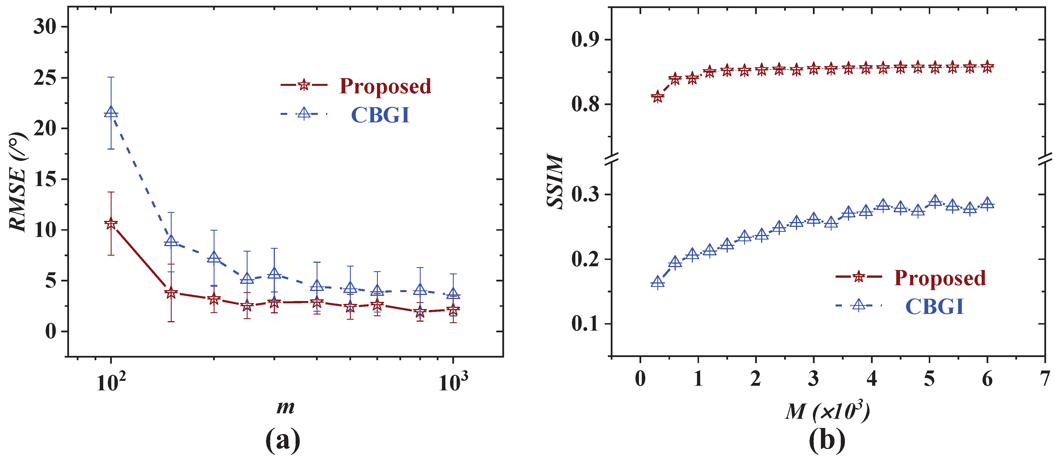
In order to make a comprehensive comparison of the different methods, the experimental results are quantitatively evaluated to compare the object location accuracy and the reconstructed image quality. At first, the accuracy of the object-locating estimation can be characterized by the rooted-mean-square-error (RMSE), written as

$$RMSE=\sqrt{\frac{1}{K}\sum _{k=1}^K\left[{({\overrightarrow{e}}_k-{\overrightarrow{r}}_k)}^2\right]}$$

(9)

where ${\overrightarrow{e}}_k$, ${\overrightarrow{r}}_k$ is the vectorized representation of the estimated and the ideal trajectory, respectively. As discussed in Ref. [13], the accuracy of the object-locating procedure could be greatly effected by the measurement number m in each image period. To get a clearer view, the RMSE of different methods is presented in Figure 3a. Here, we have to mention that, to ensure the object to be static in an image period, the moving speed of the object is also adjusted in this experiment to compensate for different number of measurements. With the increasing measurement number m, the object-locating accuracy of different methods evaluated by RMSE appears to be declining, which is consistent with the inference in Ref. [13]. Besides, compared with CBGI, the RMSE results of CS combined with the centroid estimation converges to a lower limit, which indicates a higher accuracy of object locating in our implementation. The better performance can be explained as, when the moving object is assumed to be sparse, the goal of CS reconstruction is to recover the sparse object from the sensing matrix corrupted by the unsparse noise. Once the background noise is suppressed, the accuracy of the centroid estimation could also be enhanced.

Secondly, the reconstructed image quality is evaluated by the widely-adopted structural similarity index (SSIM) [22], which considers the similarity between the image structures and the differences of image brightness and contrast at the same time. As shown in Figure 3b, the image quality of reconstructed images are both gradually improved with the increasing total measurement number M. The results of the method based on CS combined with the centroid estimation possess a better visual quality than those of the CBGI, and the high performance can be attributed to the characteristics of CS, since it exploits the sparsity prior to suppress the background noise, which not only improve the reconstructed image quality, but also benefit the accuracy of the the centroid estimation.

In addition, we also perform our experiment to estimate the rotation angle of a rotating object using the second-order moments of the reconstructed images. The angular speed of the rotating object is also set to be reciprocal to m, e.g., when $m=200$, the rotating speed of stepping motor is set to be ${10}^{\circ }$/s, and when $m=400$, the speed is $5^{\circ }$/s, and the ideal objects corresponding to different rotations are shown in Figure 4I. For comparison, the normalized GI reconstructions are shown in Figure 4II with a fixed measurement number $m=400$ in each image periods, and the images are seemed to be degraded by the rotational motion blur. To tackle this problem, the CBGI method is also applied to estimate the rotation angle $\varphi$. Similarly, CBGI calculates the cross-correlation matrix between two blurry images reconstructed at different image periods and then rotate one of the images to find a maximum correlation. As shown in Figure 4III, CBGI could effectively estimate the rotation angle of the object, and the reconstructed image quality is increased with the measurement number, while the visual perception is still not satisfactory. From Figure 4IV, it can be easily observed that the reconstruction quality of the proposed method is better than the other methods under test, especially in the under-sampling cases. Besides, the proposed method could also accurately extract the rotation angle of the object, and effectively compensate the rotational blur caused by the rotating object.

The quantitatively comparison of reconstructed image quality and accuracy of rotation estimation by different methods is shown as Figure 5. By comparing the reconstructed images with the ideal rotating object, the RMSE and SSIM are calculated and presented in Figure 5a,b, respectively. In general, the experimental results demonstrate that the rotation angle estimation and reconstructed quality of the proposed method is superior to the performance of CBGI in our implementation. In particular, the reconstructed image quality of the proposed scheme converges to its upper limit in the under-sampling cases, which suggests a great potential of the proposed method applying in the conditions of limited number of measurements.

Further more, there is a positive regularization parameter $\tau$ controlling the sparsity constraint in CS, which may affect the performance of the image reconstruction or the estimation accuracy of the object location or rotation of our proposed method. To evaluated the sensitivity of $\tau$ on the reconstructed image quality and estimation accuracy, experiments with respect to the various $\tau$, in the case of object translation and rotation are conducted. In our experiments, three groups of data with measurement number $m=$ 100, 200, 300 are chosen to compare the different effect of $\tau$ on imaging and tracking the translational object. The location estimation accuracy evaluated by the RMSE, and the reconstructed image quality evaluated by SSIM is presented in Figure 6a,b, respectively. Likewise, the performance comparison on the case of rotational object is presented in Figure 6c,d. Overall, there exists an optimal $\tau$ that achieves the best performance on the tasks of image reconstruction and the translation or rotation estimation, but the optimal value varies under different conditions. Different from the suggested value in Ref. [21,23], the optimal $\tau$ would change with the measurement number m, and the trend is that the smaller the measurement number m, the larger the optimal $\tau$. The reason can be interpreted from Equation (4), in which the first term fits the measured data to reconstruct the image vector T, and the second term controls the sparsity of T. Generally speaking, the $\tau$ should be set in accordance with the noise level, i.e., a larger $\tau$ put more emphasis on the sparsity of object, thus the unsparse image noise could be suppressed more effectively, and a small $\tau$ is the reverse [24]. Therefore, in each image period, when the measurement number m is small, the first term of Equation (4) cannot find a good solution of T, and it requires a larger $\tau$ to suppressed the random statistical noise for a faithful image reconstruction. On the other hand, when the m is enough for the first term of Equation (4) to fit the T well, it is suggested to reduce the $\tau$ to preserve more fine details of the object.

4. Discussions

The effectiveness of the proposed method relies on the assumption that, during a limited number of measurements, the moving object can be regarded as immobile [7,13]. So we can infer that, if the object is moving fast and the sampling rate of the camera is low, the number m of the measurements to meet our assumptions would be limited to a very small value. In reverse, if we have a camera with a moderately high sampling rate, we would have a much greater tolerance for the moving speed of the object. Moreover, in our experiment, we consider that the frame rate of the camera is limited to 200 fps, so the number of measurements m to satisfy our assumption is also finite. If the number of measurements in each image period is not set properly, it may result to an inadequate sampling or some additional motion blur.

For example, as shown in Figure 7I,II, when the speed of the horizontal translational moving object is set to be 0.65 mm/s, and the frame rate of the camera is 200 fps, the reconstructed image quality first increase with the number of measurements, and then decrease due to the appearance of the motion blur. Similarily, in Figure 7III,IV, when the rotating speed of the moving object is set to be ${10}^{\circ }/$ s, the behavior of the reconstructed image quality against the number of measurements appears a similar upward and then downward trend. It also suggests the importance to choose a proper m when the sampling rate of the camera is not high enough. Once the sampling device is fast enough, it will be more tolerant to the choice of m.

Although, there are already many outstanding deblurring methods developed to solve the motion blur in conventional imaging. It is worth noticing that, in the conventional “single-snapshot” direct imaging, the translational motion blur is usually modeled as a convolution of a clear image with a shift-invariant blur kernel, e.g., the point spread function. The commonly used methods to solve this kind of problem is applying some additional image priors, such as the global gradient distribution of the clear images [25]. Moreover, handling the rotational motion blur could be an even more difficult task, since the blur kernel is spatially variant in size, shape and values among pixels. To solve the problem, some research regards the spatially variant kernel as a weighted sum of several spatially invariant kernels [26], and makes the problem solvable. However, the motion blur model is quite different in GI, since it relies on the random modulation of the light source and only point a non-resolvable bucket detector to the object, thus the blur kernel cannot be directly and accurately analyzed. Therefore, there still exists some obstacles to be solved when introducing the noted motion deblurring algorithms into the GI scenario.

5. Conclusions

To summarize, we have proposed a simple but trustworthy method of tracking and imaging the moving object based on the reconstructions of compressive GI and the low-order moments estimation. By exploiting the sparsity constraint of CS, the proposed method would achieve the image reconstruction with a much better visual quality and less measurements than is possible using the second-order correlations. Without any pre-processing operations, the proposed method applies the low-order moments of the image to directly extract the centroid position and the rotation angle of the moving object, which takes the advantage of saving time and computation. Our experiments demonstrated that the proposed method can locate and compensate both the translational and rotational motion blur in GI with high-accuracy and high-efficiency. In addition, the proposed methods do not require much prior knowledge of the motion information, e.g., the directions or initial positions, and the experiment can be performed in a conventional GI setup without additional devices, which could benefit a practical approach for GI to observe the dynamic phenomena effectively and in a flexible manner.