1. Introduction
In these modern days, demands for delivery services are growing rapidly, especially with the growth of the e-commerce market. The expansion greatly increases demands for direct-to-customer deliveries. The last leg of the direct-to-customer supply chain, also known as the last-mile logistics, is the delivery of products from outlets to customers. Indeed, this part of logistics may incur more costs than other parts of management costs [
1] as it involves multiple aspects such as security when encountering not-at-home recipients, greenhouse gas emissions, a lack of critical mass in some areas which may require additional vehicles to make delivery and add extra costs to the courier, etc.
Urban logistics are also facing several salient difficulties such as access regulation, road restriction, parking conditions and environmental pollution [
2]. In addition to the costs of the last-mile logistics, customer services also play a major role in increasing customer loyalty, which subsequently increases company market share. The driver’s experience is another key to efficient delivery operations which result in gaining consumer preferences for logistics services. Driver’s local knowledge or expertise may also influence their decisions when there are road traffic accidents or abnormal traffic congestion in the area.
Managing last-mile logistics is indeed difficult to achieve optimum performance, especially with a large number of delivery locations. It is normal practice for managers to assign areas to a driver based on their local area experience. However, because delivery demands for each day in the assigned area may differ greatly, the driver may not be able to complete all deliveries in the area before the end of their scheduled shift. Therefore, day-to-day management should consider flexible delivery area in order to reallocate workload of a high demand zone to other zones. We denote the term vehicle time as the length of time a vehicle takes to start its journey from the depot until returning back to the depot to finish the whole day journey.
The most common problem that managers usually face in the urban logistics is unbalanced vehicle times as logistics demands change each day. A solution with vehicle time violations is referred to the case when some vehicles cannot return to the depot in time. This may result in failed deliveries and the delivery attempts must be made in the following day, adding extra cost to the total logistics operation. Therefore, the last-mile logistics planning should avoid assigning too many delivery jobs or creating too large coverage area for one vehicle.
Finding a solution to a problem of balancing vehicle time for the urban logistics is not an easy task. Ideally, one can embed the problem into the classical optimization problem with a secondary objective to minimize vehicle time variance. This additional term is a nonlinear polynomial function which is much more difficult to solve. In addition, the fact that travel times in a real-world situation depend on traffic congestion complicates the problem even further.
Traffic congestion has become a common problem in many big cities. There have been numerous reports that Bangkok traffic jams are among world’s worst [
3]. Congestion delays are very costly in logistics industries especially for those with time sensitive services such as express delivery products. The majority of traffic delays are predictable [
4]. The demand for transport at peak hours contributes directly to a large number of on-road vehicles. These predictable delays, however, may not be avoided if severe traffic congestion occurs all day—which is what happens in Bangkok. Therefore, Bangkok logistics industries utilize multiple transportation modes, such as motorbikes, vans and trucks, in order to accelerate delivery services.
Normally, routing problems consider timely and cost-effective deliveries with the shortest routes and the lowest number of active vehicles. However, for heavy traffic areas, travel times play a very crucial role in achieving an efficient and practical solution. For example, choosing a route with less traffic, more customers can be served by a single vehicle. Furthermore, the route balance is frequently considered in the courier industry for balancing the working time among delivery vehicles.
Solving a dynamic routing problem (i.e., with the whole time-dependent matrix) would require to make requests for the traffic-time distances from a point to every other point in an online manner. This can be very computationally expensive in practice for problems with a large number of customers. This aspect is of particular importance in contexts when the daily delivery requests from potential customers are not known beforehand but available in the morning, and a good decision must be made as soon as possible (within 30 min in our case).
Therefore, the goal of this research is to demonstrate the potential of using the proposed route adjustment approach to adjust a solution (given by a regular, pre-determined driver-area delivery zone) that is primarily infeasible in terms of vehicle working time. The updated solution will have fewer number of vehicles with a working time violation, and as many as possible driver’s locations in the driver-area delivery zone are retained so as to maintain the driver experience. As the process of acquiring traffic data in the urban logistics problem with time-dependent traffic information is the most time-consuming step, the proposed heuristic route adjustment method is initially applied to single time-dependent traffic information in order to reduce the overall processing time. The route time of the solution obtained with single time-dependent traffic information is subsequently updated with point-to-point actual traffic time from map services to get the actual vehicle time. In our business case studies, a vehicle working time limit is fixed due to drivers’ working hours. We found, however, that by tuning the vehicle working time parameter, the obtained route solutions could reduce the overall time violation and achieve better route balance with the time-dependent traffic information. Finally, since solution methods in the literature focused mainly on creating a new route without taking into consideration the driver-area delivery zone, those methods are not directly comparable to ours.
The rest of this paper is structured as follows. The review of related and relevant literature is given in
Section 2. A problem description is described in
Section 3. Proposed solution methods are presented in
Section 4. Numerical experiments are provided in
Section 5. Finally, we give conclusions and perspectives in
Section 6.
2. Literature Review
Urban or city logistics has been investigated for many years but evolved over time due to environmental changes [
5]. The problem is associated with freight transportation including logistics movements that allow freight to arrive at markets for producing other products and movements that are made by end-consumers [
6]. Factors involving urban logistics include the growth of city population, e-commerce, sharing economy and sustainability [
7]. Planning urban logistics has been supported by advanced technology such as automation, big data, digital connectivity and automotive technology. There were also concerns about the rapid growth of urban logistics which increased city air pollution levels [
8]. Emission reductions and sustainability were discussed in many publications such as Yao et al. [
9] who studied profits and CO
2 emission in collaborative city logistics.
Last-mile delivery, which is the last leg of the supply chain, accounts for 28% of the total delivery cost [
10]. There have been some attempts to improve the efficiency of the last-mile delivery, such as Modular BentoBox System [
11] where commodities were deposited to the bento box locations for an end-consumer to pick them up. This practice was adopted by logistics operators such as Post.24 (Austria), and SmartPOST (Estonia). Furthermore, shipment efficiency can be improved by consolidating and synchronizing shipment resources between logistics companies such as those in Singapore logistics collaboration [
11], an interactive freight-pooling service [
12], or the use of third party consolidation centers [
13]. Recently, Wang et al. [
10] proposed to increase the last-mile delivery effectiveness by applying a crowdsourced delivery model, utilizing a large pool of citizen workers to reduce infrastructure expenses.
The last-mile logistics can be considered as a vehicle routing problem. Route balancing problems are usually introduced in order to find fair job distributions amongst all vehicles. Majority of researches in the literature tackle the routing balance problem as a vehicle routing problem with two objectives. Generally, the bi-objective function includes (1) minimizing the total route length and (2) balancing other variables between routes. Examples of balancing variables can be classified into two types: load-related variables and length-related variables. For the load-related variables, there were several solution methods proposed such as an integer programming model [
14], and a mixed integer programming model [
15]. To balance length-related variables, such as total distances, the method of Jozefowiez et al. [
16] applied the min-max formulation as one of the objective functions and was solved with the non-dominated sorting genetic algorithm II (NSGA-II). The length-related variable involving a route cost was also solved by a multi-start strategy on Path-Relinking [
17]. Lozano et al. [
18] implemented evolutionary algorithms to find solutions to vehicle routes with seven balanced objective functions. A real case study on distribution of orders across Hong Kong was studied in Zhang et al. [
19] by applying multi-objective large neighborhood search to create delivery routes with profit balanced.
Clustering algorithms such as
k-means have also been applied to partition areas for a vehicle routing problem [
20]. The two-stage approach starts by applying
k-means to partition the entire problem into several areas, and the borders are subsequently adjusted to balance the number of visiting locations within clusters. While the original
k-means algorithm can partition the whole region into areas based on the visiting location distribution, the algorithm does not produce equally sized groups for the number of visiting locations. Thus, the second stage, which is a method for adjusting borders, is applied to move points from a large cluster to a smaller adjacent cluster.
While most solution methods presented above were mainly introduced for a single time period vehicle routing problem (e.g., Dantzig et al. [
21], Buhrkal et al. [
22] and Gong et al. [
23]), there has been an increasing number of researches aiming towards a vehicle routing problem with time-dependent traffic information (TD-VRP). Variation of vehicle speeds under different traffic conditions throughout the course of the day, especially in the urban area, reflects real-life complexities of a traffic congestion. In the early TD-VRP research, the problem concerned a step function travel time [
24], a probability function [
25] or a time-dependent matrix [
26]. These time-dependent properties do not satisfy the
first-in-first-out (FIFO) property—if a vehicle leaves a node
i for a node
j at a given time, any identical vehicle leaving node
i for node
j at a later time will arrive later at node
j [
27,
28]. In order to preserve the FIFO property, Ichoua et al. [
27] proposed a time-dependent model in terms of a vehicle speed in which the speed of a vehicle changes whenever the boundary between two consecutive time periods is crossed. In 2012, Kritzinger et al. [
29] adopted the travel speed model and improved the time-dependent matrix by floating car data information which contains travel time information during a 15-minute time slot from GPS probe.
To the best of the authors knowledge, so far no study has been carried out in the context of logistics planning with driver experience and time-dependent traffic information. In addition, there are only a few studies that address the practicality of using online time-dependent travel time for a large-scale problem. For example, Montero et al. [
30] applied an exact algorithm to solve instances up to 40 locations, while Kritzinger et al. [
29] applied a heuristic algorithm to Solomon’s instances with 100 locations. In the present study, we deal with two large-scale instances of problem size 609 and 978 customer locations, respectively. In addition, Gendreau et al. [
31] discussed the issue of the time-dependent logistics planning which relies on the next-generation web-based travel information technologies to provide data in milliseconds or microseconds. With today’s online mapping technologies, the map API requesting time to obtain a full time-dependent matrix itself for problems considered in this work already exceeds an hour computational time limit. Therefore, searches for the global optimal solution to a large-scale problem are not an option with existing technologies in the present study.
3. Problem Description
The last-mile logistics problem we consider in this work is a problem arising in this modern day. Each day drivers must distribute commodities to several locations. Delivery locations change daily depending on demands, and the list of locations to visit is available approximately one hour before the job assignment procedure starts. Our goal was to create a plan to utilize m vehicles to visit n locations but those vehicles should return to the depot within the time limit in order to avoid drivers to work overtime. In addition, vehicle times for all vehicles should be balanced which means the plan with lower vehicle time differences is more preferable. Finally, the plan should assign drivers to their original coverage areas as much as possible because the drivers have their own expertise in their responsible area. The drivers know shortcuts and detour routes which become very convenient when there are road incidents such as road blocks and extreme traffic congestion. Additionally, drivers gain familiarity to delivery protocols when visiting the same locations many times.
Traffic information must be considered when creating a logistics plan. The traffic information, determining a vehicle speed, can be presented by the time-dependent traffic information and can be obtained by map APIs such as Longdo Map (Thailand map and road traffic application) [
32], or Google Map. These APIs allow us to have a better travel time estimation between locations as the map providers use historical traffic information to predict road traffic congestion. For Longdo Map, the main source of the time-dependent traffic information is the data from Thai public data and GPS probes which are collected by the Thai Intelligent Traffic Information Center (iTIC) [
33]. Time estimation obtained from the application is known to be one of the best traffic estimation tools in Thailand.
To obtain traffic data, the map APIs require locations or points on Earth as a pair of longitude–latitude coordinates. Providing a request with two locations to the map APIs, we obtain travel duration of a trip between the two locations. A trip starting at a specific time is referred to as a trip instance, and is a trip with the fastest route for the time being. Collecting a trip instance for every location pair generates a travel time matrix given that a vehicle departs at time instance t. A collection of travel times for all locations for every time instance in the horizon is called the time-dependent matrix.
We consider here a logistical planning problem with the assumption that the business has existing operations. This existing urban logistics plan provides city coverage for each driver. In this way, drivers will gain more area knowledge (e.g., the local road system, traffic issues) as they get assigned to the same coverage area repeatedly. The issue with the existing plan is the fact that there are significant differences of daily workload between drivers, and the visiting locations can vary depending on the daily orders. In such cases, some drivers may have to drop visits to some locations, or work overtime.
Designing route for the last-mile logistics problem is known to be an NP-hard problem. Applying time-dependent travel matrices increases problem complexity [
34]. It is almost impossible to provide the optimal solution for a real-world problem in a very limited computation time. Another computational challenge is the time taken for making requests for travel distances and times from the map API. Normally, times to enquire the distance and travel time between two locations at a time
t is less than a second. However, the API request time grows at the order of
where
n is the number of locations. The connection times can be reduced slightly if the API has an endpoint to collect information as a batch query or a matrix query. Since each request takes approximately 15 min, the time taken for collecting a time-dependent matrix could be more than 165 min if a travel time of each trip is collected on an hourly basis between 9 a.m. and 7 p.m. as in our case.
In our courier business problems, daily delivery requests from potential customers are available in the morning, and a good decision for the vehicle routes must be made within 30 min. Taking into our consideration the conditions outlined above, we face scenarios with the following constraints:
The vehicle-zone map (i.e., city coverage area) which maps locations to vehicle zones is available.
Each location has service demands in which a driver must deliver commodities.
Each location requires a service duration of 4 min during which the assigned driver stops to make a delivery.
There is no road restriction, and vehicles can make a delivery at any location.
Travel routes or distances must be road distances.
Travel duration must consider time-dependent traffic information.
Drivers have limited working hours where drivers should return to the depot.
Deliveries can be made at any time of the day.
Vehicle times should be balanced.
Results of the final plan should match that of the original vehicle-zone map as much as possible.
4. Proposed Solution Method
In this section, we introduce a two-phase algorithm to generate route solutions for the last-mile logistics problem. The two phases of our algorithm include: initialization phase and vehicle time violation improvement phase. The first phase initializes and predetermines vehicle times from the provided city coverage area. The second phase, which is the main part of our method, improves vehicle times to avoid vehicle time violations.
Algorithm 1 presents the initialization phase. The algorithm starts by importing data inputs which include a vehicle-zone map and customer coordinates. Next, the algorithm creates mapping between customers and vehicle zones and pre-assigns the customers to vehicles according to the customer locations based on the vehicle-zone map information. Vehicle routes are generated by connecting depot to customers using the “nearest customer rule” in order to choose the next unvisited customer. This insertion method creates a route which always goes next to the unvisited customer with the shortest travel time (rather than distance). The process is iterated until all customers are visited. Finally, the algorithm calculates each vehicle time.
| Algorithm 1: Phase I: Initialization phase |
Data: Vehicle-zone map (city coverage area)
Data: Customer coordinates
Result: Initial solutions with vehicle routes and times
- 1
Import the vehicle-zone map and customer coordinates. - 2
(Mapping customers to vehicle zones.) Pre-assign customers to vehicles according to the customers’ locations using the vehicle-zone map. - 3
(Generating routes.) For each vehicle, starting from the depot, insert the unserved customer using the “nearest customer rule” which goes next to the unvisited customer with shortest travel time. The insertion will be iterated until there is no unserved customer left in that vehicle. - 4
(Calculating vehicle time.) For each route, calculate the vehicle time by summing vehicles’ travel times and service time of all customers in that route.
|
After Phase I, the travel time of some vehicles may exceed a pre-specified operating time limit required by the company. The goal of Phase II is to reduce the number of vehicles that violate the working time capacity, and as many as possible locations in the vehicle-zone map are retained.
Algorithm 2 presents the steps of Phase II, which we refer to as the route adjustment algorithm. The algorithm takes the routes and vehicle times obtained from Phase I as algorithm inputs, and creates the list containing all customer locations in those vehicles with time violations. Each customer location in the list will be mapped to the nearest target vehicle with remaining working time left (also referred to as a non-violating vehicle). Customer locations in the list are then sorted in ascending order of the travel time to the corresponding target vehicle. Starting with the first location in , if the insertion does not create a time violation in the target vehicle, the move is accepted, and the vehicle route time of both vehicles are updated. If, in addition, the updated route time of the vehicle (from which the customer location is removed) no longer exceeds vehicle working time limit, all customer locations in this vehicle will be removed from the list . This process is sequentially iterated over all the customer locations in the list until all locations are examined or the list becomes empty.
It is worth noting that since the insertibility has been checked before carrying out an insertion, the assignment will never create time violation in the target vehicle. Moreover, when the termination status for Phase II is failure, it means the travel time of some vehicles still exceed the required working limit, and most likely the provided time limit was too small. We will show later in
Section 5.4 how to set appropriately the level of working time limit to avoid such failure status.
| Algorithm 2: Phase II: Vehicle time violation improvement phase (Route Adjustment) |
![Applsci 10 07156 i001]() |
|---|
5. Empirical Case Study: Courier Company in Bangkok
In this section, we present the empirical results of our study by first working through a didactic example to illustrate in practice the approaches that we are advocating. Next, we present a real-world problem and the challenges we are facing, followed by experimental results obtained with our proposed method. We then give an analysis of the effects of assigning customers in ascending order of travel time in Phase II. Subsequently, we present the advantages of using the optimal working time limit in order to find a routing solution with balanced total working time. Finally, the transferability of a route solution obtained in a fixed time instance to the time-dependent traffic information urban logistics problem will be touched upon.
5.1. Didactic Example
Let us start with an example consisting of 10 zones.
Figure 1 contains three subfigures.
Figure 1a illustrates the original distribution of delivery locations and driver delivery zones across the service region.
Figure 1b displays the adjusted delivery zones to eliminate vehicle time violations.
Figure 1c presents a graph with lines tracking changes in violation amount when applying the route adjustment algorithm by keeping track of the adjusted working time violation of each vehicle while going through Phase II as a function of the swap number.
Initially, after Phase I, the assignment of customers using a vehicle-zone map leads to three vehicles with working time violation (those initially having positive time violation), namely, vehicle numbers 1, 3 and 9. Applying the route adjustment algorithm in Phase II (Algorithm 2), the first swap moved a customer from vehicle 1 to vehicle 5. Starting from swap 2, customers were moved from vehicle 1 to vehicle 8 until the target vehicle 8 has no available working time left. From swap 39 onward, customers from vehicle 3 were assigned to vehicle 2 until swap 71 when the target vehicle 2 was full. The algorithm continued until no vehicle has time violation using a total of 128 swaps to solve the problem. Post-adjusted assignment is given in
Figure 1b. Two untouched vehicles were vehicles 4 and 7 as the zones corresponding to these two vehicles are relatively far away from those vehicles with time violation. Another important observation is that it is possible that the working time of a target vehicle reduces after having a customer inserted. This is due to the fact that the shortest travel time according to the traffic condition between any two locations is used as a distance function as opposed to a road distance. For example, this happened at swaps 40 and 42.
5.2. Real Problems
Two real-world scenarios, Scenarios A and B, in Bangkok road network of dimensions with 609 and 978 locations are considered. The number of vehicles are 10 and 15, respectively. Service time for each customer was taken to be 4 min. Working time limit for each vehicle was set to 480 min (8 h).
Figure 2 gives the initial assignment according to the vehicle-zone map of the two scenarios.
We define a location or point as a pair of longitude-latitude coordinates. A trip or arc refers to an ordered pair of points (origin and destination). A trip instance is a trip taken at a specific time instance. Map API’s route choice for time and hence distance are calculated based on the shortest travel time method. Travel time of one trip instance can be significantly different from the other trip instance due to the traffic. Therefore, for a problem with n locations, since the reverse trip time is not necessarily same as the forward trip time, we have to collect travel times for each time instance. Collectively, these queries take roughly 15 min for one time instance.
In order to see the effect of the time instance on the routes built, and in particular on vehicle time violation, a travel time of each trip was collected on a weekday between 9 a.m. and 7 p.m. (hourly basis) with durations and distances reported in seconds and meters, leading to 11 time instances for each trip. Since the route which gives the shortest travel time may be different from one time instance to the other, we can see from
Figure 3 that distributions of the pairwise distance at different time instance is slightly different.
Figure 4 gives the mean speed of
trip instances for both scenarios as a function of time instance at which the data was collected. The reason for the plots having a near perfect parallel relationship is the vehicle types. In fact, vehicles consist exclusively of motorcycles for Scenario A, and vans for Scenario B. Since the data of both scenarios was also collected on the same day, this explains why a strong relationship exists between mean speeds of the two scenarios.
Table 1 summarizes relevant information for Scenarios A and B.
5.3. Experimental Results and Analysis
The proposed method was applied to the real-world problems in
Section 5.2. Here, we present the results of time violation reduction in our improved solutions. Furthermore, we provide comparison results between assigning customers in ascending order of travel time in Phase II against assigning customers in a random fashion.
5.3.1. Vehicle Time Improvement
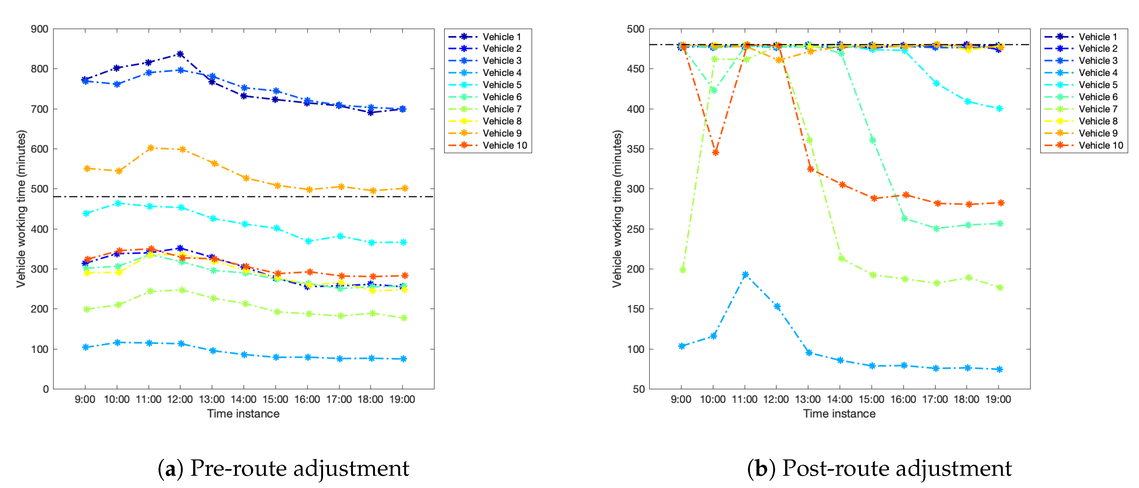
We provide a comparison of vehicle time when routes were built using different time instances.
Figure 5 and
Figure 6 give results of vehicle time of initial assignment according to the vehicle-zone map (Phase I: pre-adjustment), and the post-adjustment after the Phase II was applied on problems in Scenarios A and B, respectively. Note that values from different time instances of same vehicle are connected by the lines just for the sake of visualization. Problems with different time instance, however, are unrelated, and solved independently.
For Scenario A, regardless of the time instance used, we can see that initially three vehicles exceeded 480-min working time limit. After applying the route adjustment algorithm, all vehicles are within in the limit.
As for Scenario B, we can see from
Figure 6 that initially about half the number of vehicles exceeded 480 min of work time. After applying the route adjustment algorithm, no vehicle time violation presented except for 11 a.m. and 12 p.m. time instances where 1 and 3 vehicles violated the time limit, respectively. Let us remind that relatively slow average speeds were recorded at these two time instances (See
Figure 4).
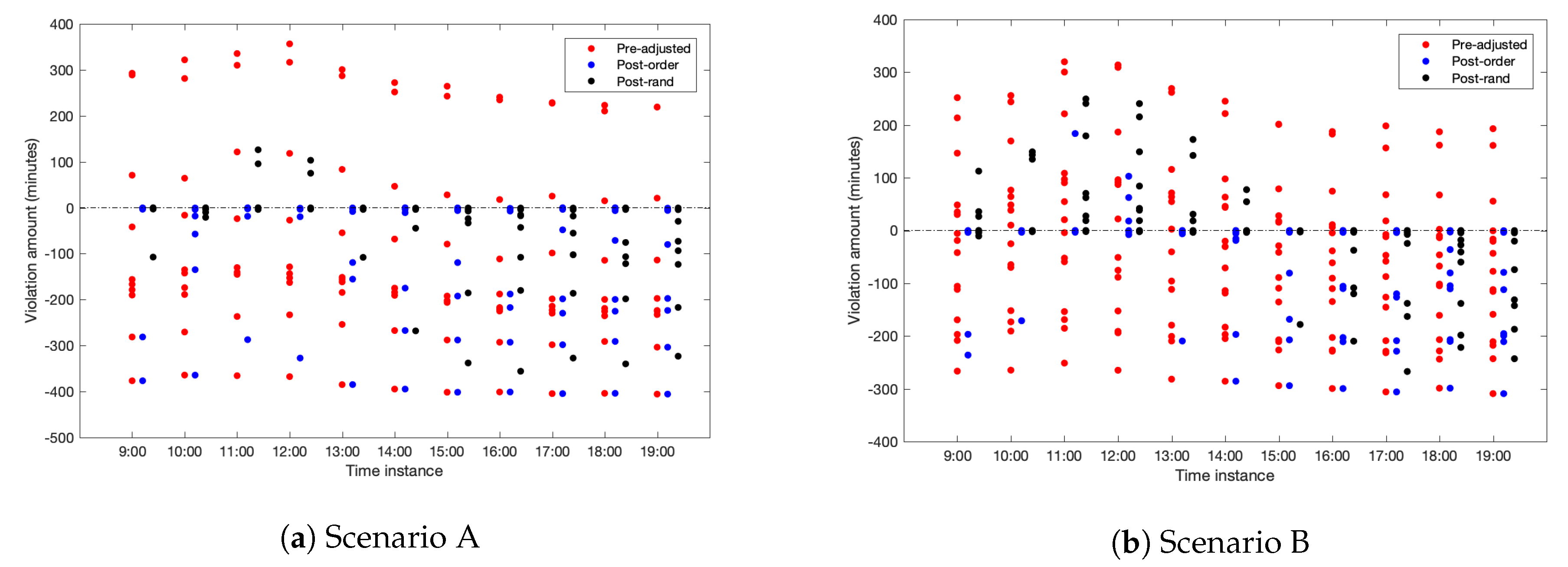
5.3.2. Effects of Assigning Customers in Ascending Order of Travel Time
To demonstrate the importance of assigning a customer in ascending order of travel time to the nearest non-violating vehicle as described in the route adjustment algorithm (Algorithm 2), we modified Step 4 of the algorithm by randomly assigning a customer from
. The results are shown in
Figure 7. The red plot shows distribution of Phase I’s vehicle violation time. The blue and black plots correspond to results obtained after going through Phase II with ascending order and random assignment, respectively.
We can see clearly that Phase II with ascending order assignment performed significantly better than the random one. While there were only two problems for ascending order assignment exiting with unsuccessful termination status (Problem B—11 a.m., and Problem B—12 p.m.), eight problems with the random assignment exited with unsuccessful termination status (2 problems in Scenario A, and 6 problems in Scenario B). In addition, the algorithm also had more remaining working time left with the ascending order assignment than that of the random version.
5.4. Towards Balancing Vehicle’s Total Working Time
Route balance is the difference between the longest and the shortest among all the vehicle working times in the problem (route time range). In the route adjustment algorithm, the vehicle working time limit has been taken as an algorithm parameter. In this section we demonstrate the importance of finding optimal working time to achieve vehicle’s total working time balance.
5.4.1. A Motivating Example
Recall from
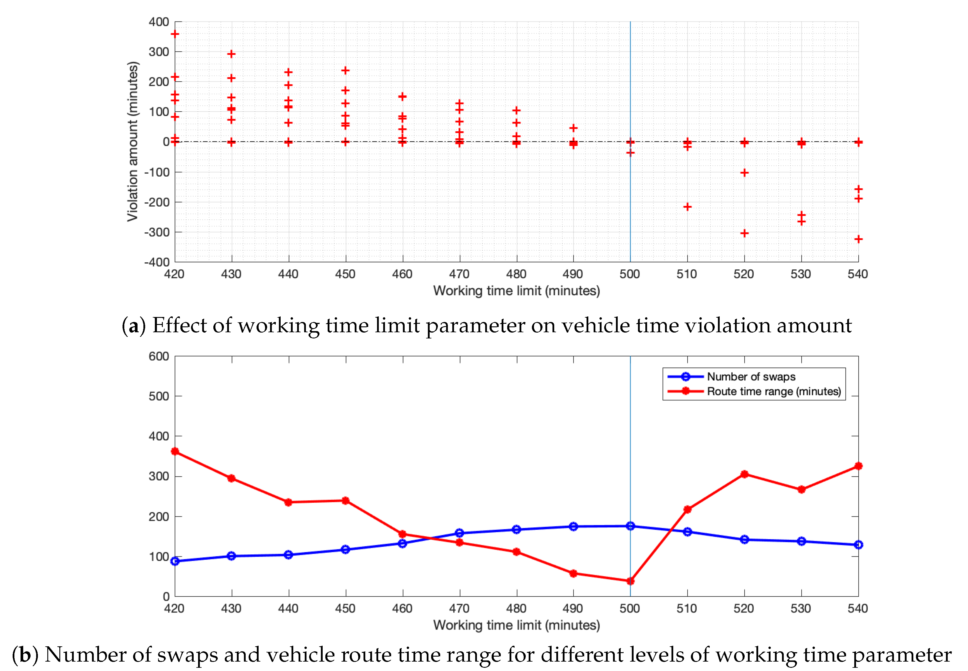
Section 5.3.1 that Phase II of Problem B—12 p.m. exited with an unsuccessful termination where three vehicles violated the working time limit. The results suggest that the 480-min time allocated may not be sufficient. To find an appropriate working time limit, we rerun Phase II (Algorithm 2) with several different working time limit parameters
on Problem B—12 p.m. The results of this experiment are given in
Figure 8. The dot plot in
Figure 8a presents the amount of violation by each vehicle. The x-axis represents the working time limit (
) set as a parameter for the route adjustment algorithm (Algorithm 2), and the y-axis represents the amount of time violation. Each cross (+) corresponds to the violation amount of each vehicle route in the solution plan. There are a total of 15 vehicles in this problem. A positive violation amount (above zero line) means that a particular route violates the provided working time limit while a negative violation amount means that the vehicle time is under the working time limit. Obviously when
, we see that three crosses are lying above the zero level violation amount. Hence, three vehicle routes (out of 15) violated the working time limit set by the company, consistent with our previously obtained result.
A few observations can be drawn from
Figure 8a. First, it can readily be seen that if we use the working time limit of 500 min as the route adjustment algorithm parameter, vehicle times are most balanced. The more we decrease (to the left) or increase (to the right) the working time limit from this point, the further away the route becomes from a balancing situation. This is demonstrated by the red curve in
Figure 8b which calculates the route balance (difference between the longest and shortest route times). Another important observation is that the number of swaps in Algorithm 2 tends to be highest at the optimal working time as shown by the blue curve. This happens because if the working time limit was set too low (to the left of the optimal duration), the route adjustment algorithm will quickly terminate with unsuccessful termination status. On the other hand, if the working time limit is too high (to the right of the optimal duration), the algorithm will also quickly terminate but this time with a successful termination status as it is easier for a vehicle to satisfy a high working time limit (hence no violation). Whenever either of the two cases occurs, only few locations will be swapped before termination.
5.4.2. Finding Optimal Working Time Limit
Define the
optimal working time to be the smallest working time limit leading to no vehicle’s working time violation. In order to obtain the optimal working time, we search for such smallest working time
for which at the end of Phase II, no vehicle violates the working time
(i.e., a successful termination status is returned). In particular, for each fixed time instance between 9 a.m. to 7 p.m., we solve an optimization problem for optimal
. Referring back to our motivating example,
Figure 8a suggests that the optimal
for Problem B—12 p.m. will lie somewhere between 490 and 500 min (transitioning from violating to non-violating situation).
Table 2 reports the optimal working time of problems in Scenarios A and B for all time instances. From the table, we see that the optimal working time for Problem B—12 p.m. is 494 min. The table gives, in addition, the percentage change in the number of resulting customer assignment from the original coverage area (vehicle-zone map). For this particular problem, the percentage change is found to be 18%. Overall the change is less than 28% and 18% for problems in Scenarios A and B, respectively. Moreover, we provide the average travel speed (in line with the plot given earlier in
Figure 4) for a side-by-side comparison in the table.
Figure 9 presents the relationship of the optimal working time
in terms of the average travel speed. We can see that the optimal working time is inversely proportional to the average speed. Therefore, the proposed Phase II has proven capable of finding a feasible solution from a solution with time violation very quickly, while at the same time preserving a certain level of customer assignment from the original coverage area.
5.5. From a Fixed Time Instance to Time-Dependent Traffic Information Urban Logistics Problems
In light of still very limited implementation and with the goal of filling in some of the research gap, we examine the feasibility/infeasibility of transferring the route solution obtained with one time instance to actual time routing case. Results in this section enable better understanding of the effect of using a pre-determined route, that was built based on a static pre-trip travel time, with the en-route real-travel-time scenario.
5.5.1. From Time Instances to Time-Dependent Traffic Information with 480-Min Working Time Limit
Now we examine the transferability of the route solution obtained earlier with a fixed time instance to the problem with time-dependent traffic information or actual traffic time. In other words, using the route solution obtained in
Section 5.3.1, we query point-to-point the actual traffic time from map API to get the actual vehicle time. Since there are altogether 11 time instances, we will retrieve and compare actual times of the routes constructed from each time instance. Results of time violation amount (from 480 min) are given in
Figure 10.
Recall from
Section 5.3.1 that for problems in Scenario A when a fixed time instance was used, no vehicle violated the working time of 480 min at any time instance. Unfortunately, using these route solutions, the retrieved actual vehicle time of almost all time instances violated the 480-min working time limit except for 11 a.m. and 12 p.m.
As for Scenario B, we saw earlier from
Section 5.3.1 that some vehicles at time instances 11 a.m. and 12 p.m. violated the 480-min working time limit. Now, using these route solutions,
Figure 10b reveals that the retrieved actual vehicle time of all time instances violated the 480-min working time limit. In addition, the amount of violations could be as much as 100 min as in the case of Problems B—11 a.m, 6 p.m. and 7 p.m.
This problem arose as the effect of the imbalance of vehicle working times. Referring back to the results obtained in
Section 5.3.1,
Figure 6b revealed that applying the route adjustment algorithm with 480-min working time limit resulted in solutions with highly unbalanced route time. Let us take Problem B—7 p.m. as an example. Although no vehicle violated the 480 min,
Figure 6b indicated that 10 out of 15 vehicles worked up to nearly 480 min, while the other 5 vehicles still had about 60–300 min remaining. Once we calculated the route time using the actual traffic time, those vehicles with nearly zero minutes of working time remaining will likely violate the working time limit of 480 min in the case of actual time. Finally, notice also the highly imbalanced working times with the time-dependent traffic information displayed in
Figure 10.
5.5.2. From Time Instances to Time-Dependent Traffic Information with the Optimal Working Time Limit
We have seen that transferring a route solution from a fixed time instance with 480-min working time limit led to a working time violation in the actual time routing problem. Now, instead of using the route solution obtained with the 480 min set by the company, we use the route solution obtained with the optimal working time
we found in
Section 5.4.2.
Figure 11 presents the actual vehicle time of the route solution built with the optimal working time (obtained from
Table 2).
For Scenario A, we can see that using the route solution constructed with any time instance, all retrieved vehicle times were below 480 min required by the company. For Scenario B, although some vehicle times exceeded 480 min, the amount of violations were less than 30 min, far below what we obtained previously in the unbalanced case (see
Figure 10). While the evidence of
Section 5.5.1 showed the impossibility of transferring the routes built with a fixed time instance to the problem with the time-dependent traffic information, the obtained results in this section confirm the transferability of the routes built from a fixed time instance to the actual traffic time problem. Eventually, the balancing property is also better retained in the actual time problem when the optimal working time
was used in place of 480 min when building the routes.
6. Conclusions and Future Work
In this work, we present an effective approach to improve infeasible solutions obtained initially with the routing coverage areas provided by a courier company. From the industry’s point of view, the improved solution having fewer number of vehicles with time violations should be acquired within a very limited computational time, and without creating significant changes to the original coverage areas. It is impossible to apply methods available in the literature which may take hours if not days to find just a feasible solution. Therefore, our proposed solution method applies a route adjustment algorithm to decrease working time violations. Our result shows that the route adjustment algorithm could remove all working time violations except for two problems of Scenario B with traffic time at 11 a.m. and 12 p.m. as the vehicle speed for the two time instances are very slow. In addition, by applying our route adjustment algorithm to get the optimal working time parameter, we found that the time violation is no longer present at any time instance, and a balanced route solution can be better achieved. Our results reveal also that the optimal working time should be set relative to the average travel speed. Furthermore, we analyze the uses of the time instance solution in the time-dependent traffic information environment. The result indicates that the improved solutions obtained with the original working time limit are still present some violations in almost every time instance (except 11 a.m. and 12 p.m. instances of Scenario A). With the optimal working time, on the other hand, the new route solutions have more improvements in terms of the number of working time violation, the amount of time violation that exceeds the original working time, as well as the route balancing. These findings indeed highlight the effectiveness of our proposed approach in solving an urban logistics problem with time-dependent traffic information. Our analysis also shows that the current vehicle fleet size is sufficient to meet the customer’s demands on the selected day. This information can be used by the business to evaluate their potential fleet expansion strategy in the future when vehicle time constraints are regularly violated.
Finally, our present work enlightens some research directions. For example, it is possible to consider a meta-heuristic method as an alternative to the greedy insertion in the route adjustment algorithm. In addition, integrating time-dependent traffic information within the route adjustment algorithm may also encourage a better approximation to the final result. For the latter, the study should pay attention to the computational time and data enquiry time reduction aspects.


