A Convolutional Neural Networks Based Method for Anthracnose Infected Walnut Tree Leaves Identification

Abstract

Anthracnose is a fungal disease that infects a large number of trees worldwide, damages intensively the canopy, and spreads with ease to neighboring trees, resulting in the potential destruction of whole crops. Even though it can be treated relatively easily with good sanitation, proper pruning and copper spraying, the main issue is the early detection for the prevention of spreading. Machine learning algorithms can offer the tools for the on-site classification of healthy and affected leaves, as an initial step towards managing such diseases. The purpose of this study was to build a robust convolutional neural network (CNN) model that is able to classify images of leaves, depending on whether or not these are infected by anthracnose, and therefore determine whether a tree is infected. A set of images were used both in grayscale and RGB mode, a fast Fourier transform was implemented for feature extraction, and a CNN architecture was selected based on its performance. Finally, the best performing method was compared with state-of-the-art convolutional neural network architectures.

1. Introduction

Fungal diseases pose a major problem in agricultural environments, especially in orchard and horticulture crops production. When trees suffer from infections, the production of the crop diminishes substantially and the economic impact can be catastrophic [1]. As part of precision agriculture, automatic plant disease detection and classification can alleviate this problem, with unsupervised early detection systems that could identify the presence of disease on the leaves of the trees and classify them appropriately for planning any precautionary measure or action to be taken. The rise of machine learning (ML) in the past years has significantly boosted the progress in this research area [2,3,4,5].

Several studies can be found in the bibliography regarding machine learning approaches for image-based plant disease identification. Leaf disease detection in various types of leaves and diseases has been investigated by classic ML algorithms, such as, support vector machines (SVMs) [6] and back-propagation artificial neural networks (ANNs), achieving 88–92% accuracy [7].

The feed forward neural network (FFNN), learning vector quantization (LVQ) and radial basis function networks (RBFs) with accuracy range 56.7–90.7% [8], advanced deep residual neural networks that acquired 96% accuracy [9], as well as deep learning (DL) methods, such as convolutional neural networks (CNN), that were able to achieve 96.3% accuracy [10].

In terms of advanced CNN architectures, a series of achievements have been reported, including the identification of 13 types of plant diseases with an accuracy range of 91–98% [11], the identification of 58 different diseases for 25 types of plants with accuracy up to 99.53% [12], and some meta-architectures of CNN (AlexNet, GoogleNet) also implemented resulting in the same accuracy over 14 crop species and 26 types of diseases [13]. The size and variety of the leaf-image dataset on advanced CNN structures has been investigated in [14], leading to the conclusion that large and diverse datasets critically improve the performance of the models. In some studies, alternative imaging approaches are investigated, such as triple channel convolutional networks [15], and the combination of visible, thermal and depth imaging fungus detection on tomato leaves [16]. Other studies focus on specific combinations of plants–disease, such as cucumbers–anthracnose, downy mildew, powdery mildew and target leaf spots [17], apple trees-mosaic, rust, brown spot, alternaria leaf spot [18], apple trees/black rot with four severity stages by [19], brinjal (aubergine)/bacterial wilt, cercospora leaf spot, tobacco mosaic virus by [20], banana trees-sigatoka and speckle [21], wheat/wheat stripe rust, wheat leaf rust, grape downy mildew, grape powdery mildew [22] and tomato leaves–gray mold, canker, leaf mold, plague, leaf miner, whitefly, powdery mildew [23].

In our study, we aim for the anthracnose disease identification on walnut tree leaves, with images that were taken in real conditions. An investigatory analysis takes place by testing and evaluating various architectures of CNNs, as well as the effect of color in images, and the use of fast Fourier transform (FFT) as an additional feature extractor.

2. Methodology

Our approach on classifying anthracnose-infected leaf images focuses on the recognition of marks that appear (brown-yellowish in red green blue (RGB) images) on the leaf as spots or surrounding its perimeter, as seen in Figure 1.

Deep learning methods such as convolutional neural networks (CNNs) are applied in order to train a classifier to distinguish images with leaves containing the infection, and leaves which are healthy. CNNs are using convolutions and pooling operations on an image in order to transform the image in a way that will enhance desired features. This process creates several images where their impact is constantly optimized, and the images with the most useful features are given higher weights in the final model. These built-in operations give CNNs the advantage compared to other algorithms in the task of image classification. Therefore, CNNs have been outperforming vanilla artificial neural networks (ANNs) or support vector machines (SVMs), which were state-of-the-art up until the time CNNs were introduced [24]. On top of that, a fast Fourier transform (FFT)-based pre-processing technique is implemented for feature extraction on the images. Lastly, an optional background removal method is used in order to evaluate the effect of background on the performance of the classifier. These methods are analytically described in the following subsections.

2.1. Process Description

The process followed in this study is shown in Figure 2. There are three stages: The preprocessing stage, where the images are gathered, prepared and finally split; the machine learning (ML) stage, where the images are used to train a classifier and allow it to self-improve until it reaches its maximum potential; and the predictions stage, where characterized test images are provided to the classifier to evaluate its actual performance. The stages are presented descriptively below.

2.1.1. Pre-Processing

• Load the dataset: The images are loaded recursively based on their pathnames. Depending on the prefix of their filename, a label value of ‘0’ or ‘1’ is appended to each loaded image, explained in detail in Section 2.3.
• Color conversion: Two functions for color conversion were implemented in this study: a conversion from the BGR to the RGB color-space, where the order of the image’s color channels changes to the most common (RGB) format, and a conversion from BGR to the grayscale color-space, where the images lose all the color information and maintain only the brightness and saturation for each pixel.
• Feature extraction (only for grayscale): For the grayscale images, there is additionally applied a feature extraction method, the Fast Fourier Transform (FFT). This method helps bring out the edge features of the leaves, thus potentially improving the performance of the model compared to a straightforward approach of grayscale images.
• Background segmentation (optional): This method removes the background from images with the use of thresholding, dilation and erosion, as commonly used methods in computer vision.
• Data normalization: The dataset values are normalized within the (0, 1) range in order to ensure that the loss function, which is usually not convex, finds the global minimum as easy as possible. Reducing the range of input values also assists the convergence of the backpropagation algorithm.
• Dataset shuffling: The dataset is being shuffled by Python’s “random.shuffle” method, which is an order-shuffling algorithm based on a random number generator. After the application, the order of the images, which originally was alphabetical, is now mixed throughout the dataset.
• Dataset splitting: The dataset is being split in the following fashion: First, 15% of the total dataset is held out and set as the testing set, then the remaining dataset is split again in the 80/20 fashion, where the small portion is used as the validation set. The rest is used for training the algorithm. The training and validation sets are used for the training of the algorithm, while the testing dataset is used only after the classifier is trained, in order to make predictions.

2.1.2. Learning Process

• Convolutional Neural Network (CNN) architecture definition: The architecture of the CNN is defined based on experimentation and trials. The number, type and order of layers is the important aspect that can lead to effective network architecture.
• Functions definition: Various functions that are used throughout the network are being defined through bibliographic research and trials. We carefully choose the activation function, which is the function that defines the output of the layer, and the loss function, which is the function that is used for the optimization of the network’s weights.
• Training: This is the process where the algorithm tries to create a function that describes the desired relation, based on the training data. It then makes predictions based on this function and moves to the next step.
• Validation: Following the previous step, the function that the algorithm created is being evaluated against the validation dataset. The error in the predictions is being calculated, and the algorithm tries to find a way to minimize this error. This part defines the “learning” of the process.
• Finalizing the model: The training-validation process repeats itself until the algorithm cannot improve itself anymore. When the training loss and the validation loss have become almost the same, lowest-possible value, and before the validation loss starts to increase, we stop the procedure and finalize our model.

2.1.3. Prediction

• Test the CNN based on trained data: The performance of the finalized model is measured by its validation accuracy; i.e., the accuracy it could achieve based on the data that it has been given to train and evaluate. This is indicative of the model’s performance, but the real performance is only evident when predictions on unknown data take place.
• Make predictions on the test data: We use the testing data, which is completely unknown to the model, to make predictions on each image’s class. For each image, the classifier provides a predicted class, which is stored alongside its true class.
• Calculate performance metrics: This is the final step where the predicted classes are being cross-checked over the true classes of the testing images. Then, the testing accuracy, precision, recall and f1-score of the model are calculated. A confusion matrix is also used in order to visually evaluate the performance of the model, and also check if it is biased over any class.

After the performance metrics are calculated, they are stored, and the algorithm returns to the shuffling of the original dataset, and continues the process. For the particular approach, the algorithm runs a total of five times, and finally the mean value of the performance metrics are being calculated. The reason why we perform this loop is to ensure the stability of the model and eliminate outliers that are not representative.

2.2. Data Acquisition

Classification of images is a complex process that needs large amounts of feature-rich data, and a good self-trained algorithm in order to be able to classify correctly. A Sony RX100 II with a F1.8 (T) lens was used to take photos of raw format 5.472 × 3.648 pixels resolution, of the walnut trees located in the orchard under various lighting conditions. Specifically, photos were taken during morning, noon and afternoon times, having the sun across or behind the camera. This detail is important because the position of the sun affects the diffusion/refraction of light through/on the leaf, and creates a difference of how anthracnose is captured on the image; as dark brown spots on a light green leaf or light brown spots on dark green leaf. The leaves were manually cropped and split into categories. A total of 4491 images of leaves, both with and without anthracnose, were gathered from a walnut crop field located in the Volos region, Greece. The anthracnose-infected leaf images amounted to 2356, which is slightly more than the healthy leaf images which amounted to 2135. In Figure 3a,c we can see an indicative image from a leaf infected with anthracnose, with and without background, and in Figure 3b,d, a healthy leaf again with and without background.

2.3. Data Preparation

Since all images had different proportions, their size was modified to a 256 × 256 pixels proportion. This resolution was deemed satisfactory for both maintaining the images features, as well as keeping computational time to a minimum.

All images were originally saved in an RGB 3-channel, and small script was set up in order to assign a numerical value as a label to each image, according to its prefix. Therefore, images which had “anthracnose_” as prefixes were assigned with the value ‘0’, and images which had “healthy_” prefixes were assigned with the value ‘1’.

The images are loaded into the memory alphabetically due to their order in the containing folder, as well as the script used to load them. If we split the dataset as is in training/validation/testing, it is certain that at least the training and testing datasets will not contain sufficient or any images from one or the other class. For example, if the testing set derives from the last images of the loaded dataset, the set will only contain healthy images, therefore we will not be able to measure the performance of the classifier correctly. Therefore, since the order of the images was defined by the name of each file, a shuffling method based on a random-number generator is used to randomly reorder the images so that the sampling is as unbiased as possible, thus avoiding improper training.

2.4. Data Split

The dataset was split into three sections: A training portion dedicated to train the classifier, a validation portion that would allow the training process to improve, and a testing (held-out) portion which is a part of the dataset that is completely hidden from the training process and will be used for validating the classifier on unknown data. All splits create subsets that contain a 50/50 ratio of healthy and anthracnose-infected leaves photos in order to avoid the unnecessary bias that would incur if a dataset would contain images from only one category.

Python’s random.shuffle generator was used to shuffle the order of images and avoid having datasets with similar external conditions. This way, images of leaves with different shapes, angles, levels of infection, main leaf color, brightness, ambient lighting, etc., are all included in all categories in order to achieve the highest possible variability. Variability in the datasets ensures that the model will be trained in the most generalized fashion possible, and will be evaluated and tested under all conditions [25].

The first data split takes place by removing 15% of the total dataset and saving it for later use as testing. The remaining 85% of the dataset is then split again into an 80/20 ratio, resulting in the following portions, as seen in

Table 1. Data splitting percentages and purpose.

Dataset	Training	Validation	Testing
% of total dataset	68%	17%	15%
# of images	3053	764	674

.

The validation set is used during the training process in order to help the algorithm update its weights appropriately, so that it can improve its performance and avoid overfitting. After the model has finished training, we run in on the testing data, and verify if it has classified the test images correctly, thus creating the need to keep the testing set hidden.

2.5. Performance Metrics

In this paragraph, we describe the performance metrics that were used to evaluate the performance of this study. In general, the performance metrics are used in order to provide a common measure of the performance of the trained classifier, against new images from the testing set. The outcome of this prediction, in comparison to the actual class label that was assigned to the image, can take one of the four values, true positive (TP) or true negative (TN) if it is classified correctly, and false positive (FP) or false negative (FN) if it is misclassified.

These values are then used to calculate the performance metrics that are most commonly used in classification problems. In

Table 2. Performance metrics used in our study.

Name	Description	Formula
Accuracy	ratio of correctly predicted observation to the total observations (preferred in balanced datasets)	(TP + TN/TP + FP + FN + TN)
Precision	ratio of correctly predicted positive observations to the total predicted positive observations	(TP/TP + FP)
Recall	ratio of correctly predicted positive observations to all observations in actual class	(TP/TP + FN)
F1 score	is the weighted average of Precision and Recall (preferred in unbalanced datasets)	[2 · Recall · Precision]/[Recall + Precision]

we present the performance metrics used in our study for evaluation of the performance of our classifier, together with their descriptions, as well as their mathematical formula.

Additional to the performance metrics, we choose to visualize the prediction results in confusion matrices. The confusion matrix is a table that displays the aforementioned values in such a way that one can easily view the number of properly classified examples, as well as false positives and false negatives. In our study, which is a binary classification, the confusion matrix is of size 2 × 2. The template used for the confusion matrix is shown in

Table 3. The confusion matrix template.

Confusion Matrix		Predicted
		Anthracnose	Healthy
True	Anthracnose
	Healthy

.

All the confusion matrices with the results for each tested scenario are located in the Appendix A of this paper.

Finally, a loss function (or objective function, or cost function) is used to evaluate how well the specific algorithm performs on the given data. In our study, we used the mean squared error (MSE), where the average squared difference between the estimated values and the real values is calculated during the training. It always has non-negative values and it is preferred, because large errors create larger consequences than equivalent smaller errors.

The value of the loss function is important for the evaluation of the model’s performance, because it can show us if the model can improve its performance and how well the predictions correspond to the real values. The closest that this value is to 0, the better will be the performance of the model.

2.6. Feature Extraction Preprocessing with Fast Fourier Transform

Fast Fourier Transform (FFT) is used in image preprocessing for the easy detection of abrupt changes in images, such as the presence of anthracnose in leaves. The image is considered as a signal described in a two-dimensional spatial domain. Abrupt changes in images are mainly considered as high-frequency signals. As a result, image representation in the frequency domain is a powerful tool for the detection of such changes, so that they can be enhanced or removed, depending on the required task. Moreover, applying filters to images in the frequency domain is computationally faster than to do the same in the spatial domain. Similar applications of the FFT combined with ML algorithms have been tested in image classification applications of different domains with promising results [26].

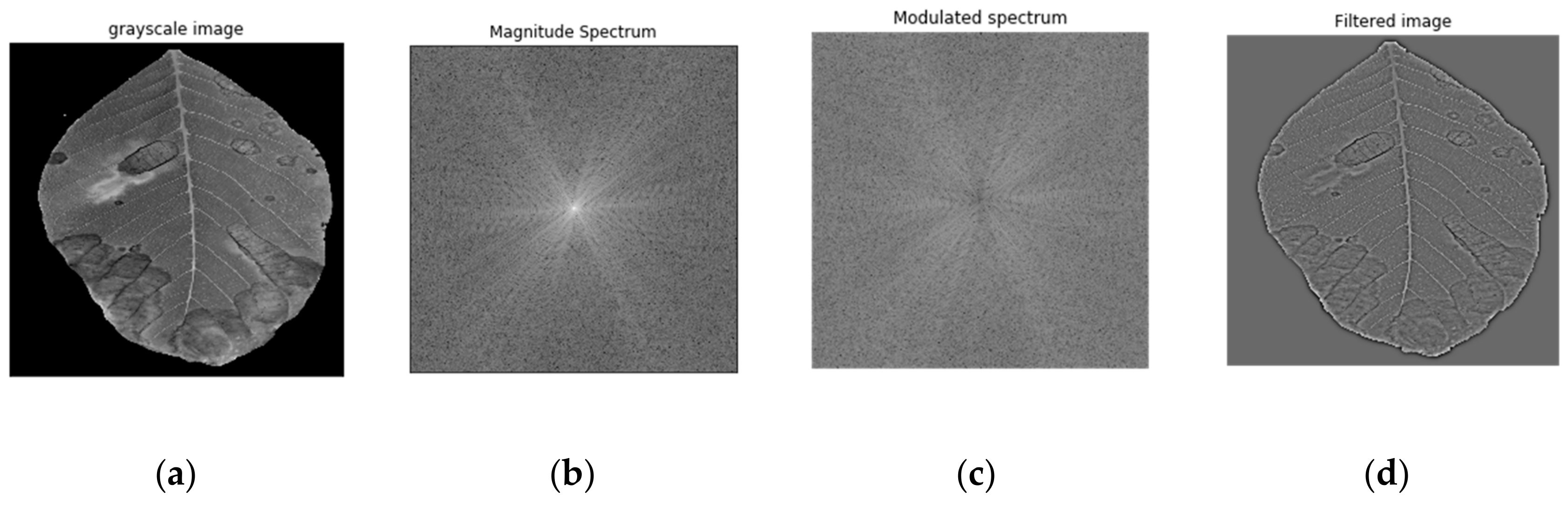
FFT is applied on an anthracnose-infected leaf image (Figure 4a) and decomposes the signal into its periodic components in order to produce their frequencies. After the implementation of FFT the image is converted from the spatial domain to the frequency domain. Each point represents a specific frequency contained in the original image. After the FFT application, the image is shifted in such a way that the DC-component F(0,0), which corresponds to the average brightness, is displayed in the center of the image.

The next step is to calculate the magnitude of the Fourier Transform, as it contains most of the information of the image structure. More specifically, if the magnitude changes abruptly, the signal is considered to be high frequency. Figure 4b shows the magnitude spectrum after the implementation of FFT with the pixels in the center of the image representing its low frequencies. In general, anthracnose is considered as an abrupt change, and is consisted of high frequencies. As a result, a high pass filter which allows only high frequencies should be implemented. Since the low frequencies are near the center of the Fourier image, a radius around the center is determined, and all the frequency components within that radius are constricted. For that reason, each image gets multiplied by the Gaussian high pass filter where a smooth cut off process is used. The cut off frequency is considered to be equal to the standard deviation σ in the frequency domain, and is equal to 0.3.

The magnitude spectrum after the use of the filter where the low frequencies were successfully removed, is shown in Figure 4c. Finally, the inverse Fourier transform was implemented in order to obtain the original image without low frequencies, as it is shown in Figure 4d.

The choice of simple FFT over wavelet transforms or more advanced techniques is because the time domain is irrelevant to the particular problem. The photographed leaves have no temporal information, therefore we need only to focus on the frequency precision, and FFT is the most appropriate method for this application [27].

2.7. Convolutional Neural Network Architecture

For our study, we built a deep neural network that utilizes convolution and pooling operations, which have proven to be very effective on problems regarding image classification. Classic feature extraction techniques, used in computer vision, required the manual feature selection in order to find the appropriate feature to utilize. Convolutional Neural Networks (CNN), a subcategory of Artificial Neural Networks (ANN), can do this automatically by applying multiple filters on the input images, and then learn to select the ones that are necessary for the images’ proper classification.

A typical structure of a CNN is to start with a convolutional layer, followed by a pooling layer, repeating this combination as many times as necessary, continuing with one, or more fully-connected layers, before ending with the final output layer. Additionally, a dropout layer can be added after either a dense layer, a fully connected layer, or a pooling layer.

In our implementation we built a deep-layer network with five convolutional–pooling layers, a dense layer followed by a dropout layer, and finally, the output layer with one node since it is a binary classification. A layout of the network’s architecture along with the layers’ shapes and the number of trainable parameters, is given in

Table 4. The selected convolutional neural network (CNN) architecture.

Layer (Type)	Output Shape	Param #
conv2d_1 (Conv2D)	(None, 254, 254, 32)	896
max_pooling2d_1 (MaxPooling2)	(None, 127, 127, 32)	0
conv2d_2 (Conv2D)	(None, 125, 125, 64)	18,496
max_pooling2d_2 (MaxPooling2)	(None, 62, 62, 64)	0
conv2d_3 (Conv2D)	(None, 60, 60, 128)	73,856
max_pooling2d_3 (MaxPooling2)	(None, 30, 30, 128)	0
conv2d_4 (Conv2D)	(None, 28, 28, 256)	295,168
max_pooling2d_4 (MaxPooling2)	(None, 14, 14, 256)	0
conv2d_5 (Conv2D)	(None, 12, 12, 512)	1,180,160
max_pooling2d_5 (MaxPooling2)	(None, 6, 6, 512)	0
flatten_1 (Flatten)	(None, 18,432)	0
dropout_1 (Dropout)	(None, 18,432)	0
dense_1 (Dense)	(None, 512)	9,437,696
dense_2 (Dense)	(None, 1)	513
Total params: 11,006,785
Trainable params: 11,006,785
Non-trainable params: 0

. A more detailed figure of the proposed CNN is presented in the Appendix A.

The images enter the network at a 256 × 256 pixels dimension. The first (input) convolutional layer consists of 32 filters (kernels) of size 3 × 3, always followed by a max-pooling layer of size 2 × 2, which chooses the maximum value of each consecutive four (2 × 2) pixels. Each next convolutional layer doubles the numbers of filters (32 → 64 → 128 → 256 → 512), just like the following max-pooling layers. After the convolution and pooling operations, a flattening operation transforms the 2-dimensional matrices, to 1-dimensional arrays in order to run through the hidden, fully connected (dense) layer with 512 nodes. Following, a dropout layer drops randomly 20% of the learned weights in order to avoid overfitting. Last is the output layer with one node, since we are dealing with binary classification.

The activation function that is used in all convolutional and fully connected (dense) layers is the rectified linear unit (ReLU) and the final activation function is the sigmoid function. The algorithm is set to train for 100 epochs, however an early stopping function prevents the network to over-fit by stopping its training when the validation loss starts to increase and diverge from the training loss. For the loss, the binary cross-entropy function is calculated with an Adam optimizer [28], and accuracy is used as the measurable metric. For the model training, the ImageDataGenerator class [29] was used, offering augmentations on images such as rotations, shifting, zoom and flips.

2.8. Visualization of Convolutions

Even though CNNs are considered “black boxes”, there is a way to visualize some of the computations that take place, as well as their effect on the input image at each step. Here, we present some of the filters that are being applied at each layer, as well as the activation maps that are produced after the convolutions.

2.8.1. Filters

The filters are mathematical kernels that are being applied on the matrix that represents the image. In computer vision applications, they are constructed in such ways so that when they are multiplied with the image values, they bring out specific features, such as edges. In our study, we use a CNN with five convolutional layers (

Table 5. Filter dimensions for each convolutional layer.

Layer	Filter Dimensions	Number of Filters
Conv2d_1	3 × 3	32
Conv2d_2	3 × 3	64
Conv2d_3	3 × 3	128
Conv2d_4	3 × 3	256
Conv2d_5	3 × 3	512

).

While for the grayscale images the filter application is straightforward, for RGB images, each channel has its own filters being applied. A visual representation of the filters for an RGB image is shown in Figure 5.

These filters are important for the machine learning processing, since they bring out features of the images that will be used for the proper classification.

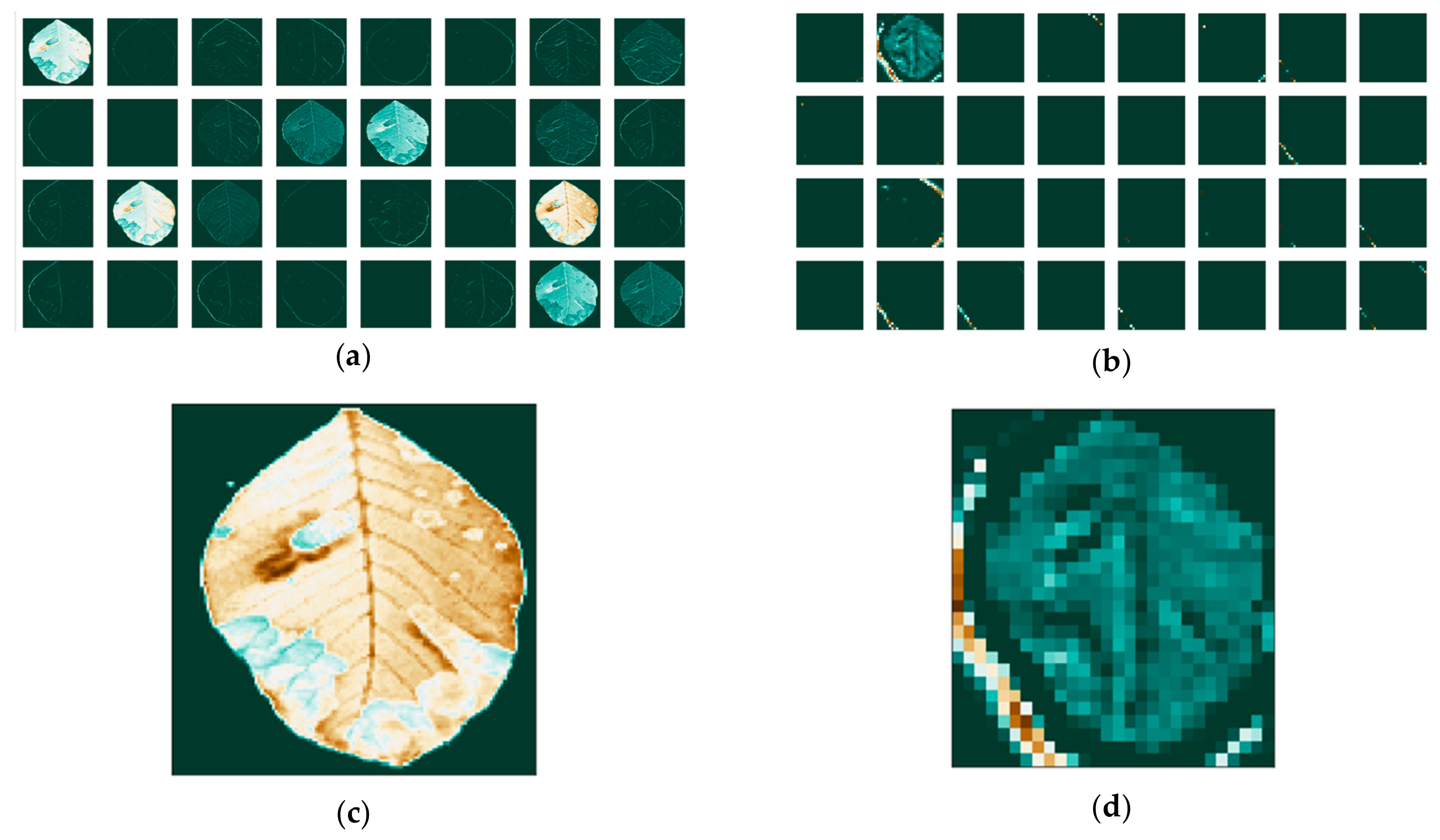
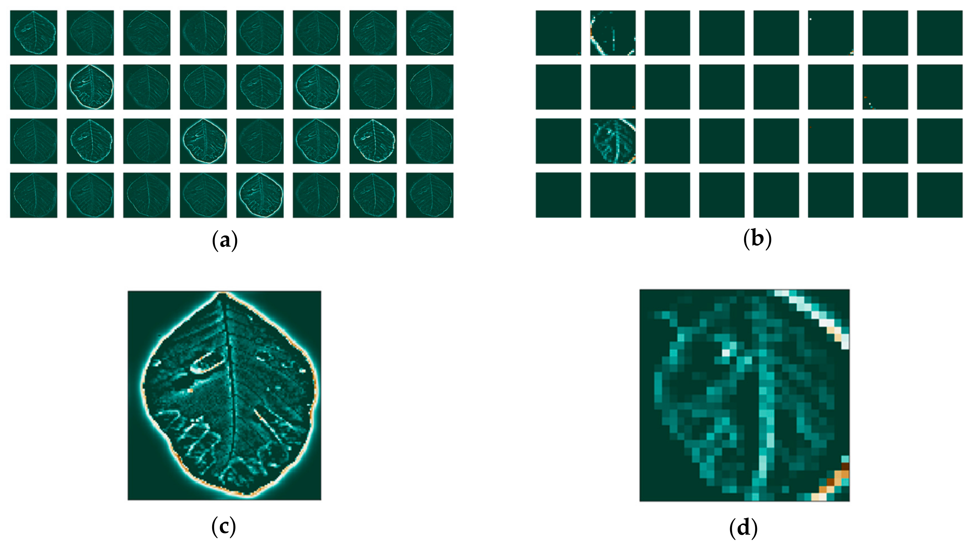
2.8.2. Activation Maps for RGB

The activation maps are the result of the filter application on the input image or on other activation maps when they enter the convolutional stage. These maps highlight features of the image that can potentially be useful for the classification. We present two cases of the activation maps of a leaf infected with anthracnose, one with the background information present, and one with the background removed. The two images are shown in Figure 6.

Since the images go through various transformations via mathematical operations, it is useful to see how the activation maps look like after the first and after the last convolutional layer. Activation maps for the leaf image that contains background information are shown in Figure 7, while activation maps of the leaf image that had its background removed are shown in Figure 8.

We can also investigate how the filters affect each channel of the RGB images independently. First, we split the image into each channel, and then we create three separate images, as shown in Figure 9.

We then apply the filters and visualize the activation maps for each image on the first and last convolutional layers of our network. The separate feature maps of each RGB color are presented in Figure 10 for the red channel, in Figure 11 for the green channel and Figure 12 for the blue channel. We notice that the filters have different effects on the different channels, obvious both in the first layer, as well as the last.

2.8.3. Activation Maps for Grayscale

We apply the same methodology on three categories of the grayscale images in Figure 13 and the images that have been transformed with the FFT method in Figure 14.

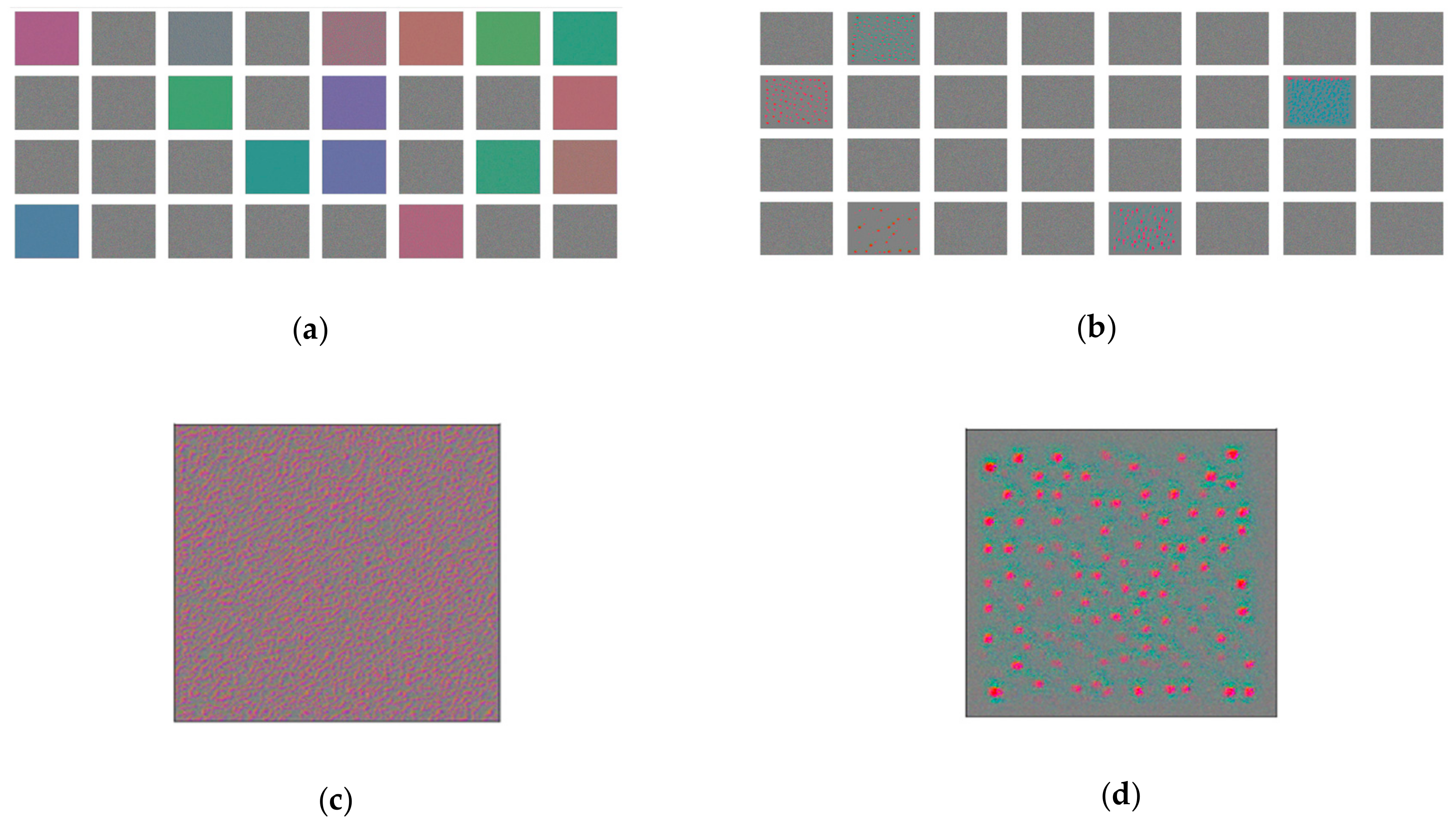
2.8.4. Filter Effect on Images

We can examine the effect of the filters by visualizing the optical pattern of the filter itself, both on a white image, and on the image of the leaf. This is done by applying gradient ascent to the input image, in order to maximize the response of the particular filter. We apply the filters of the first and last convolutional layers on a blank image, just to visualize the filter itself, as shown in Figure 15.

Following this, we then use as input the image with the anthracnose-infected leaf and see the effect of the filters on the leaf image itself, as seen in Figure 16.

This way, we can have some insight into the depths of the deep neural network, and specifically how the convolutions affect the features of an image that contains leaves.

3. Results

The Jupyter Notebooks [30] interactive computing product under the Python programming language was used for encoding the whole process, with the neural network being programmed with Keras (with Tensorflow backend [31]). In addition, the data normalization, data splitting, confusion matrices and classification reports were being programmed with Sci-Kit Learn, while OpenCV was used for loading and manipulating images, SciPy was used for the FFT application, Glob was used for reading filenames from a folder, Matplotlib was used for plot visualizations, and finally Numpy was used for all mathematical and array operations. The script was run on an Intel® Core™ i7-6950X CPU @ 3.00GHz × 20, and the CNN was trained on a Nvidia Titan GeForce GTX 1080 Ti. The computation times ranged between 15’ to 100’ per training, depending on the different input, with the grayscale images requiring the lowest training time and the RGB images requiring the longest training time.

Before starting with the exploratory analysis of the optimal CNN setup, it is necessary to see where the other famous classification ML algorithms stand in the particular problem. In a previous work [32], it was shown that neural networks outperform other algorithms in a similar dataset, thus pointing to investigating the best neural network implementation. However, some of the most famous classical ML algorithms were tested on this new dataset for the comparison. The results are shown in

Table 6. Comparison of classical machine learning (ML) algorithms.

	Decision Trees	Random Forest	Ada-Boost	Support Vector Machines	Artificial Neural Networks
Accuracy	64.59	79.55	77.45	81.37	83.38
Precision	0.65	0.80	0.78	0.81	0.84
Recall	0.65	0.80	0.77	0.81	0.84
F1 score	0.65	0.80	0.77	0.81	0.84

.

Again, it is shown that ANNs perform better in a particular problem, and therefore our choice of focusing on CNNs is justified and validated.

The first comparative analysis was dedicated to measure the accuracy as well as the loss of both the validation and the testing dataset for images containing background information. Measuring accuracies allows us to see if the predictions made to the unknown set match the performance of the model while training. In

Table 7. Accuracy and loss for the validation and testing sets, for the three preprocessing algorithms, on images with background information.

	Accuracy		Loss
	Validation	Testing	Validation	Testing
Grayscale	92.869	92.469	0.192	0.197
Fast Fourier	93.153	92.938	0.198	0.176
RGB	96.847	95.969	0.086	0.111

the accuracy percentage and the loss for each method used are listed.

The second comparative analysis was to measure the accuracy and loss for each method, but with additionally applying the background removal method. This way, the images contain less relevant-to-the-infection information, which should lead to increased performance. In

Table 8. Accuracy and loss for the validation and testing sets, for the three preprocessing algorithms, on images without background information.

	Accuracy		Loss
	Validation	Testing	Validation	Testing
Grayscale	95.710	95.469	0.116	0.130
Fast Fourier	96.591	96.531	0.108	0.105
RGB	99.006	98.719	0.031	0.049

we see that indeed by removing unnecessary information, the performance of each model has increased.

More results such as training and validation plots and confusion matrices are presented in the Appendix B.

Finally, we select the best performing model, being the one using RGB images with background removal, and compare it to state-of-the-art CNNs for image classification. These CNNs are specifically selected for comparison, since they set new accuracy records when originally trained on the Imagenet [33] database. In detail, we used DenseNet121 [34] a version of DenseNet (Densely Connected Convolutional Networks) that is 121 layers deep. Despite its depth, DenseNet managed to solve the problem of vanishing gradients, having both 1 × 1 and 3 × 3 convolutional layers, as well as batch normalization in its architecture. Another architecture we used is VGG16 [35], a version of VGG (Visual Geometry Group). Generally, in VGGs there are only 3 × 3 convolutional layers which are stacked on top of each other. ResNet50 [36] is the 50-layer deep version of ResNet (Residual neural Network), an exotic architecture that is based on “network-in-network” micro-architectures. Due to global average pooling, instead of fully connected layers, the size of ResNet50 is significantly smaller than VGG16. Finally, Inception V3 [37] is Inception’s third instalment, and is 48-layers deep. Inception V3 incorporated RMSProp optimizer and 7 × 7 convolution in the 1 × 1, 3 × 3 and 5 × 5 convolutions which were already presented within the same module of the network.

For our comparison, we use them together with their weights, and retrain only the last layers for our specific dataset, something that is called transfer learning. Thus, each algorithm is re-trained/fine-tuned on our dataset, with the same preprocessing functions, in order to compare only the models’ performance. Additionally, the training times of each algorithm have been measured with the %%time function of Python under a Jupyter Notebook. This function affects only the cell where it is called from, and was set to measure the execution time of only the training of the model and none of the preprocessing or the processing of the predictions. The results are shown in

Table 9. Comparison of most common CNNs with the proposed CNN.

	VGG16	DenseNet121	ResNet50	Inception V3	Proposed CNN
Validation accuracy	96.875	99.049	98.505	99.290	99.006
Validation loss	0.096	0.033	0.050	0.027	0.031
Testing accuracy	95.781	96.577	98.363	99.375	98.719
Testing loss	0.120	0.071	0.067	0.013	0.049
Execution time (s)	1391.31	1866.893	1290.42	1712.213	989.185

.

We notice that the proposed CNN architecture has performed better than the rest of the state-of-the-art architectures, except Inception V3, which achieved better accuracy both in the validation dataset, as well as in the testing dataset. A significant difference between the proposed architecture and the others, is that the proposed CNN is significantly shallower compared to the others, therefore it can be trained a lot faster on the same dataset.

It is clear that the proposed network achieves a similar accuracy to the state-of-the-art Inception V3 network, in less time due to its shallower architecture. The tradeoff is in favor of the proposed network, since the difference in time is significant, while the accuracy difference is minimum. Given that in this particular problem the useful features are not so complex, the proposed CNN performs satisfactorily.

4. Discussion and Conclusions

The problem of the automatic identification of anthracnose on walnut tree leaves has been tackled with the use of deep learning algorithms, specifically convolutional neural networks. A total of 4.491 images was acquired, balanced in terms of healthy and infected leaves depictions. A number of pre-processing techniques, such as fast Fourier transform and background removal, were tested in order to evaluate their contribution to the increase of performance.

Several CNN architectures were tested, with accuracies ranging from 92.4% to 98.7%, leading to the one that performed best under all pre-processing scenarios.

The proposed methodology was designed from the ground up in order to address the specific issues of the anthracnose–detection problem. Initially, we needed to address the background issue, and investigate whether or not the background plays any role in the accuracy of our classifier. Another issue that needed addressing was the type of images that we would process, meaning if they would be colored or monochromatic. Colored images contained the color information, which is important in this specific use case, since anthracnose discolors areas of the green leaf into brown spots. However, there is value in the monochromatic approach, since the images can be taken in different times within a day (or night), and the color variations might change. Monochromatic images can create a more generalized classifier, even if the accuracy appears to be lower, because it diminishes this color dependency. Because of the reduced accuracy of the monochromatic approach, a feature extractor was selected and tested on its performance. The fast Fourier transform indeed improved the results of the monochromatic approach by extracting edge information with a high pass filter, leading to clearer view of the leaves’ abrupt changes on their surface.

The best performing algorithm was then compared with a series of state-of-the-art CNNs commonly used for image classification problems. We note that our algorithm for the particular problem performed equally, and in some cases even better, compared to these algorithms. This study validates the premise that CNNs are algorithms that can offer high accuracy in image classification-based problems. This has a direct application on precision agriculture where the automatic identification of diseases is crucial for the crops.

The main outcomes of this study can be summarized as follows:

• The proposed CNN method exhibits outstanding performance when RGB analysis is performed for the examined images of this case study. This can be emanated from the fact that the results produced from the application of the CNN architecture are based on distinct features that appear specifically on the anthracnose-infected leaves, compared to the healthy leaves, i.e. brown spots and areas.
• The fast Fourier transform method seems to be of major significance in feature extraction in the case of the grayscale images, because it accentuates the abrupt changes and edges of the leaves. This denotes that the infected leaves have more edgy features than the healthy ones.
• The proposed CNN architecture exhibits high performance in all scenarios in which it has been tested considering the case of anthracnose disease identification on walnut tree leaves. As it is observed from Table 7 and Table 8, the accuracies range from 92.4% to 98.7%.
• The proposed CNN architecture exhibits better, or similar, performance to well-known CNN architectures (i.e., DenseNet121, VGG16, ResNet50 and InceptionV3) which have been efficiently used as benchmarks in image processing problems for the past years.
• Overall, for the purpose of image analysis and classification, the CNN methodology is proved to be proper for complex image classification tasks, such as the one under hand here, when a large number of images is considered, outweighing the popular CNN architectures for image analysis, such as DenseNet121, VGG16, ResNet50 and InceptionV3.

Future plans include the further investigation of the proposed architecture with images collected by infrared, near-infrared and RGB cameras, as well as with images taken at all times of day and in all kinds of weather. This will help us build a more robust classifier that will be even more invariant to external conditions. Additionally, the algorithmic part of this study will be focused towards the development and application of hybrid algorithms that utilize fuzzy cognitive maps in convolutional neural networks in order to integrate experts’ knowledge on this problem.

The aim is to increase furthermore the accuracy of the model while simultaneously offering interpretability to the classification process.