Quantum-Based Analytical Techniques on the Tackling of Well Placement Optimization

Abstract

The high dimensional, multimodal, and discontinuous well placement optimization is one of the main difficult factors in the development process of conventional as well as shale gas reservoir, and to optimize this problem, metaheuristic techniques still suffer from premature convergence. Hence, to tackle this problem, this study aims at introducing a dimension-wise diversity analysis for well placement optimization. Moreover, in this article, quantum computational techniques are proposed to tackle the well placement optimization problem. Diversity analysis reveals that dynamic exploration and exploitation strategy is required for each reservoir. In case studies, the results of the proposed approach outperformed all the state-of-the-art algorithms and provided a better solution than other algorithms with higher convergence rate, efficiency, and effectiveness. Furthermore, statistical analysis shows that there is no statistical difference between the performance of Quantum bat algorithm and Quantum Particle swarm optimization algorithm. Hence, this quantum adaptation is the main factor that enhances the results of the optimization algorithm and the approach can be applied to locate wells in conventional and shale gas reservoir.

1. Introduction

In oil and gas industry, to maximize productivity, optimization of well placement is one of the most important issues in the field development process. The optimization techniques, based on contemporary research works on this field, can be indexed in three major categories. They are (i) classical methods, (ii) non-classical methods, and (iii) hybrid methods [1]. In the early novel research endeavors, focuses were mainly shown on classical methods to tackle well placement optimization problem and among them mixed-integer programming (MIP) [2], gradient-based finite difference method [3], multivariate interpolation algorithms [4], simultaneous perturbation stochastic approximation method [5,6], and steepest ascent method [7] are significant. However, the gradient-based techniques might get trapped in local optima, which is one of the biggest bottlenecks of the gradient-based techniques. Moreover, the calculation of the gradients is complex. Hence, due to the nature of the well placement optimization problem, it is hardly solved by gradient-based techniques. On the other hand, derivative calculations are not required for non-classical methods, and less likely to get trapped in local optima than classical techniques [8,9,10]. Due to the robustness and parallelism nature, nonconventional methods with gradient-free approaches are more considered for well placement optimization. To make a model robust, consideration of risk management is important. Again, due to different heterogeneity in conventional and shale reservoirs, the production is different [11,12,13]. Hence, different search space will be produced that can be challenging for an optimization technique and the results may not be consistent. Unconventional reservoirs are relatively tight, exhibit strong heterogeneity, low permeability (<0.1 md), and possess a complex micropore structure, thus restricting the effective economic development of oil and gas. Boost up oil production from unconventional reservoirs is different from conventional reservoirs as it requires advanced technologies of multiple horizontal wells and multi-stage hydraulic fracturing. Due to the fact that in these unconventional reservoirs, the space between cracked wells is narrowed, the economic equations also need to take into account the effects of natural fractures and well interference through fracture communication. Smaller intervals connect more existing fracturing, creating a complex fracturing network during hydraulic fracturing [12,13]. Hydraulic fracturing has been widely used in many regions. Despite having many economic benefits it can damage the formation and can reduce the production rate and recovery efficiency [14,15,16]. In the operational performance, formation damage is a profoundly important issue [16]. Nowadays, most reservoirs are facing pressure reduction due to the high production rate of hydrocarbons, which leads to low recovery efficiency [15]. During the drilling operations, ineffective implementation of drilling fluid damages the reservoir formation [14].

Nonconventional nature-inspired gradient-free methods such as artificial bee colony (ABC) [17], improved harmony search (IHS) [18], genetic algorithm ([19,20], covariance matrix adaptation evolution strategy (CMA-ES) [21], differential evolution (DE) [22], cuckoo search (CS) [23], bat algorithm (BA) [24], ant colony optimization (ACO) [25], and imperialist competitive algorithm (ICA) [26], etc. have been applied in well placement optimization problem. Although these types of global optimization algorithms can provide better solutions than traditional techniques, they are still heavily affected by parameter tuning and tend to be trapped in a local optimum. To improve this situation, hybrid techniques are realized in different ways in different research aspects. In some aspects, researchers prefer to blend non-conventional techniques with classical methods [27], whereas in some cases incorporating two or more nonconventional approaches are used for developing a hybrid algorithm [28]. Following this methodology, many researchers combined different algorithm’s best features and developed many hybrid strategies ([29,30]) that showed superior performance in well placement optimization problems. However, this type of technique often lacks theoretical studies to support the proposed combination. Again, when the comparison aspect is considered DE is better than particle swarm optimization (PSO) and CMA-ES [31]. According to Reference [32], gravitational search algorithm (GSA) is superior than genetic algorithm (GA). Again, Hybrid differential evolution and particle swarm optimization (HPSDE) is compared with DE and PSO and found to outperform DE and PSO [33]. In addition, PSO provided more net present value than GA in another study [34]. Again, ACO-GA-PSO have shown superior performance than PSO, GA, S-PSO, and RS [25]. Furthermore, BA has provided better net present value than GA and PSO [24]. The performance of ICA is compared with SPSO and SCGA and the tuned ICA has outperformed other algorithms [26]. The above-stated comparison between algorithms does not establish a single algorithm as a superior algorithm. Moreover, the compared algorithms are not consistent, and a wide set of existing algorithms is not considered in the previous study.

Again, because of the reservoir heterogeneities [35,36], the nature of the cost functions is discontinuous, high dimensional, and nonconvex, which contains multiple local optima. In addition to that, due to the excessive amount of computational expenses, parameter tuning requires a substantial amount of reservoir simulations. Hence, the trial and error approach to find the best configuration is impractical. This can be attributed to the optimization algorithms erratic performance. Again, because of the lack of study in exploration and exploitation analysis, the selection of proper strategy is difficult. Furthermore, in most cases, only one reservoir is utilized to evaluate the performance of the algorithms. Such an approach does not establish the superiority of the algorithm in this field since reservoir heterogeneity changes the surface of the search field. Moreover, the result of the techniques can differ with respect to the nonlinearity, dimensionality, and surface of the search field. Previous research shows that only a few algorithms are used for comparison purposes [37]. Hence, a wide range of algorithms should be evaluated in a common synthetic reservoir to claim the superiority of a particular algorithm. Furthermore, metaheuristic algorithms are stochastic. So, statistical analysis and certain criteria should be considered to establish a technique in this field. In addition, the large search space having high dimensionality is rarely reliable for stochastic algorithms. Therefore, perceiving an efficient algorithm with an inherent ability to execute this complex optimization problem is profoundly significant.

To the best of our knowledge, there have been no researches on the application of quantum computation to deal with well placement optimization problem. Therefore, in this study, to resolve the problems mentioned before, quantum-behaved bat algorithm (QBA) and quantum particle swarm optimization (QPSO) are implemented and compared with a wide range of established algorithms. Moreover, collecting the end result in terms of cost function value does not help to fully understand the internal behavior of the algorithms. Hence, this study attempts to explain the internal behavior of the algorithms on well placement optimization with graphical illustrations.

This paper is ordered in the following manner: Section 2 is dedicated to discuss the problem statement of well placement optimization. In Section 3, we discuss the proposed techniques in detail. The comparison of different optimization methods and their analysis are provided in Section 4. Section 4 focused on the statistical and convergence analysis of different metaheuristic algorithm’s results as well as critical findings with discussion. This section also focuses on dimension-wise diversity analysis. The concluding remarks for well placement optimization are provided in Section 5.

2. Governing Equations

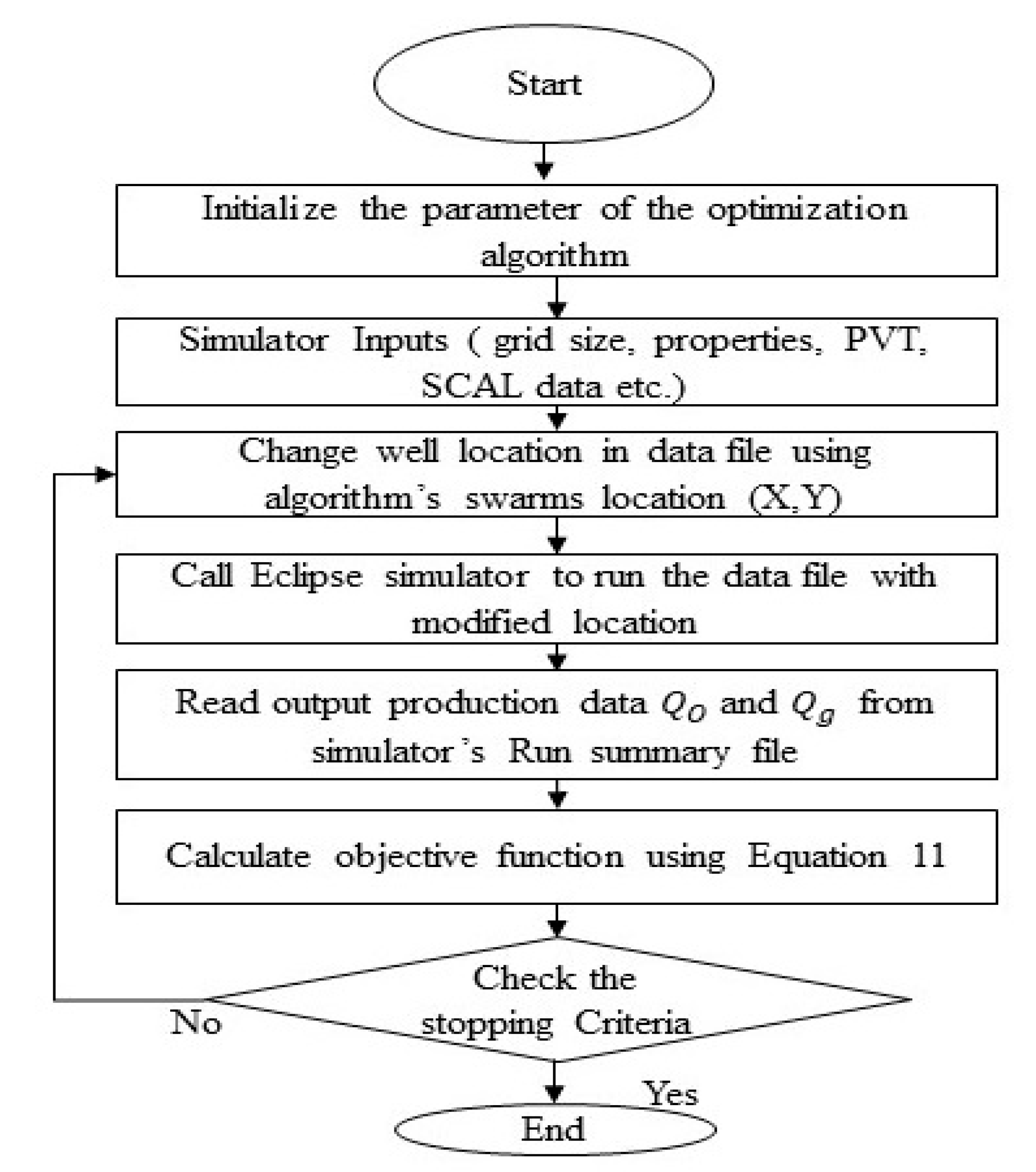
An oil reservoir’s dynamic behavior can be described by coupled spatiotemporal differential equations. In the case of a two-phase oil reservoir, these are [38]:

$$\frac{\partial }{\partial t}\left[\epsilon \frac{S_f}{B_f}\right]+q_f-\nabla [\frac{k{r}_f}{{\mu }_f{B}_f}\mathrm{K}(\nabla P_f-{\rho }_f\frac{g}{g_c}\nabla Z\left)\right] =0$$

(1)

where, ${\mu }_f$ is the viscosity of phase f (f = 0 for oil and f = w for water), $\epsilon$ is the porosity, ${\rho }_f$ is the density, $B_f$ is the formation volume factor, K is the absolute permeability tensor, $S_f$is the saturation, $k{r}_f$ is the relative permeability, $P_f$ is the pressure, and $q_f$ is the flow from ($+$ve for out, $-$ve for in) the reservoir$.$ In mathematical analysis and modeling, the relative permeability of each phase is generally described using:

$$k{r}_o=k{r}_o^0{\frac{S_o-S_{or}}{1-S_{wr}-S_{or}}}^a,$$

(2)

$$k{r}_w=k{r}_w^0{\frac{S_w-S_{wr}}{1-S_{wr}-S_{or}}}^b,$$

(3)

where a and b present the exponents in Corey’s correlation,$S_{wr}$ and $S_{or}$ are the residual water and oil saturations, respectively, $k{r}_w^0$ and $k{r}_o^0$ are the end-point relative permeabilities for water and oil, respectively.

The pressure and saturation of the oil and water phases are interrelated by the equation:

$$P_c=P_o-P_w=f\left(S_o{S}_w\right),$$

(4)

$$S_0+S_w=1;$$

(5)

where $P_c$ is capillary pressure, $P_o$ and $P_w$ are oil and water pressure, and $S_0\mathrm{and} S_w$ presents oil and water saturation.

Then, the flow rate at the wellbore can be defined using the following well production equation (IPR or Inflow Performance Relation):

$$q=\mathsf{\Psi }(kr/\mathsf{\mu }B\left(P-BHP\right).$$

(6)

where $\mathsf{\Psi }$ is the connection transmissibility factor for wells and the Bottom Hole Pressure (BHP) is determined by the Vertical Flow Performance (VFP) curve:

$$BHP=THP+\rho gL+\mathsf{∆}P+\mathsf{∆}p.$$

(7)

Among them, $\mathsf{∆}P$ presents the frictional pressure drop through well tubing, $\mathsf{∆}p$ is the pressure drop due to the acceleration, L represents the depth of the well, and $\rho$ is the density of the well production, and $THP$ is tubing head pressure. For a given well chain and termination type, the total flow, the water/oil ratio (gas/oil ratio), and the inlet/outlet pressure determine the pressure drop in Equation (7).

The prime motivation behind well placement optimization is to make sure that the expenditure remains minimum while maximizing the net present reaches the maximum value. Well placement optimization, in general, can be formulated as:

$$MaxR\left(u^n\right)$$

(8)

$$R\left(u^n\right)=NPV\left(u^n\right)$$

(9)

Subjected to:

$$LB\le u^n\le UB\forall nϵ\left(0,1,2,3\dots \dots N-1\right),$$

(10)

where $u^n$ represents well coordinates, $NPV$ presents net present value, $LB$ and $UB$ are lower bound and upper bound of the reservoir, respectively.

Net present value (NPV) changes randomly with the change of coordinates of the well location. Eclipse simulation was used to calculate the cumulative oil production, cumulative gas production, cumulative water production’s value based on the coordinates of the well location. The variables used in Equation (11) are depicted from Reference [1]. Hence, $NPV$ for a reservoir model can be formulated as:

$$NPV\left(u^n\right)={\displaystyle \sum }_{i=1}^T\frac{Q_O{P}_O\left(u^n\right)+Q_g{P}_g\left(u^n\right)-Q_w{C}_w\left(u^n\right)-OPEX}{{\left(1+D\right)}^i}-CAPEX$$

(11)

where $P_g$ denotes gas price, $Q_w$ presents cumulative water production, D is the discount rate, $Q_g$ is cumulative gas production, T is the number of years passed since the production has started, CAPEX is the capital expenditure, $P_O$ presents oil price, $C_w$ denotes cost per unit volume of produced water, OPEX is the operational expenditure, and $Q_O$ is cumulative oil production. Equation (1) constitutes an exact conventional as well as shale gas reservoir model, which cannot be solved analytically. Hence, by using complex commercial simulators like ECLIPSE, CMG to solve Equation (1) to Equation (7), production data $Q_O$ and $Q_g$ in Equation (11) can be found. Figure 1 depicts the general flow chart to acquire NPV value.

In general, Figure 1 shows the flow of the program to search the maximum net present value. At the start of the program, the parameters of the algorithm are initialized. Then, the program inserts a generated location in the data file. After that, the program calls eclipse and eclipse provide run summary file for a given location. The program will extract production data $Q_O$ and $Q_g$ from run summary file and calculate NPV.

3. Methodology

Metaheuristic algorithms are stochastic and non-deterministic. There are various types of metaheuristic methods like local search, simulated annealing, Tabu search, variable neighborhood search, population-based or trajectory-based search, etc. Besides, among all the Metaheuristic search algorithms, one of the most popular algorithms are—gravitational search algorithm (GSA), particle swarm optimization algorithm (PSO), crow search algorithm (CSA), genetic algorithm (GA), differential evaluation (DE), and bat algorithm (BA), etc. Quantum-based optimization techniques were applied in several complex engineering applications using quantum parallelism mechanisms. For multimodal optimization applications, the study of Ross indicated that quantum behaved algorithm is superior to existing metaheuristic algorithms [39,40]. Another study found that quantum computation can manage highly non-linear multimodal optimization problems naturally [39]. Again, PSO searches linearly. On the other hand, QPSO’s next position depends entirely on the probabilistic approach [41]. In QBA, the position of each bat depends on the mean best position. The quantum-behaved bat and mean best position lead local search to jump out of local positions [42]. Hence, QBA can easily avoid local optima. Since these properties are important to tackle multimodal well placement optimization problem, QPSO and QBA are discussed in the following section.

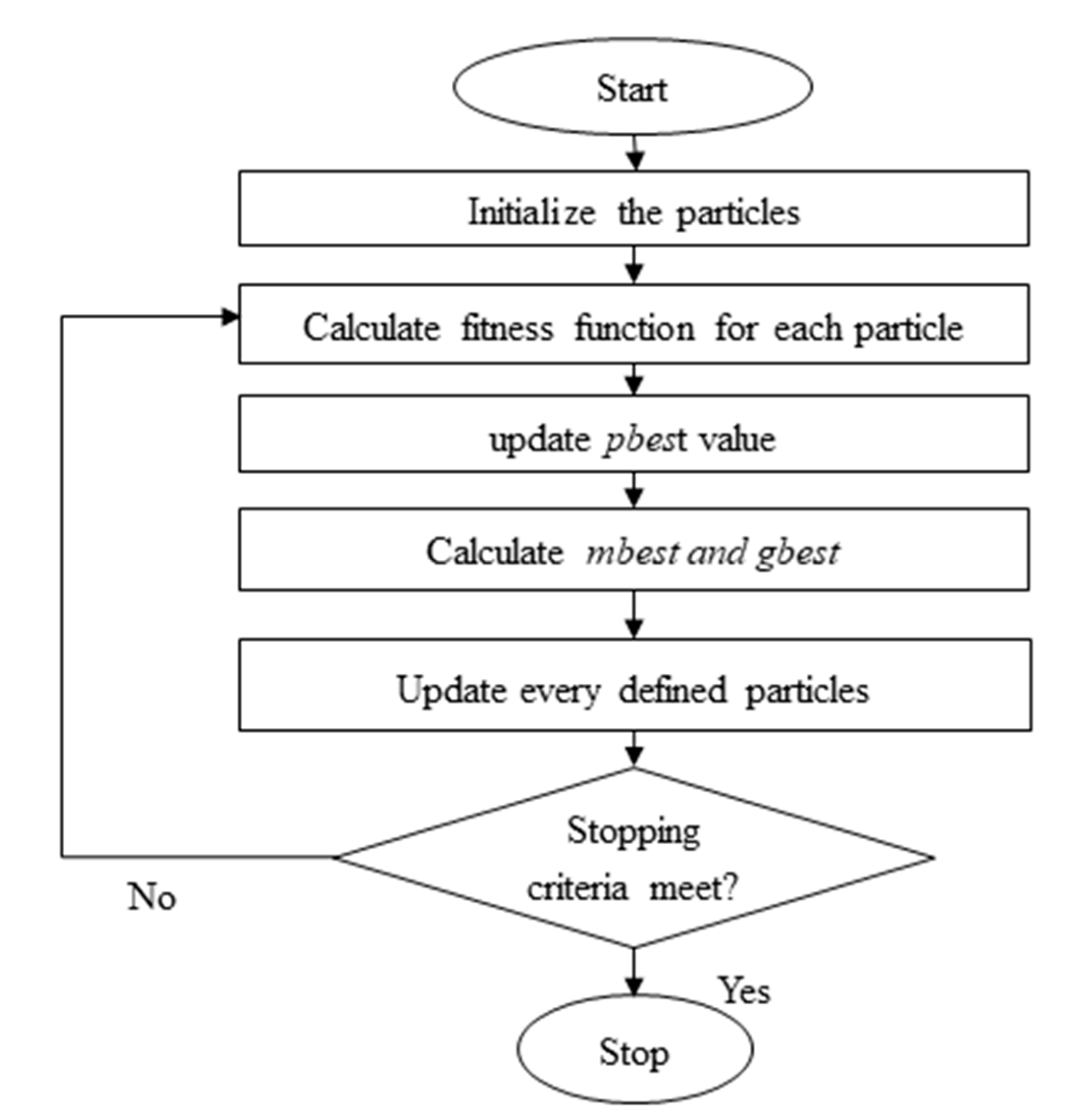
3.1. Quantum Particle Swarm Optimization Algorithm

In 1995, a novel search approach was developed and proposed by Kennedy and Eberhart [43], which is known as PSO and was stochastic. In a search space, the particles of PSO can fly and change their position with respect to time. At first, the initialization of individuals is done through a random process.

To update the velocity of each particle, the following equation is utilized

$$V_i^{k+1}=w{V}_i^k+c_{1}ran{d}_1\left(pbes{t}_i^k-x_i^k\right)+c_{2}ran{d}_2\left(gbes{t}^k-x_i^k\right),$$

(12)

where the individual i particles velocity is denoted by $V_i$ for iteration k. For defining a particle’s acceleration, $c_1\mathrm{and}{c}_2$ are introduced as acceleration constant, w is used for weight vector, $ran{d}_1\mathrm{and}ran{d}_2$ are the random number ranging from 0 to 1, for individual i position is represented by $x_i^k$ in iteration k, $pbes{t}_i^k$ and $gbes{t}^k$ denotes the best position and global best of individual i in k iteration. In the search space, by using the following equation, each particle’s next position will be updated:

$$x_i^{k+1}=V_i^{k+1}+x_i^k.$$

(13)

Sun et al. [44] implemented the principle of quantum mechanics with basic PSO. The QPSO algorithm not only tackles the drawbacks but also preserves the good features of the PSO algorithm [45], and thus the incorporation of improved search capability in addition to fast convergence is possible [46]. Another feature of QPSO is that it has only one parameter that needs to be tuned. The flowchart of QPSO is depicted in Figure 2. Figure 2 shows that at first the positions are randomly generated. Then, the cost function is calculated for each particle. Based on the results, mbest and gbest are updated. The search process will continue unless the termination criteria are met.

Unlike the behavior of the Newtonian particle that is described by both the position ($\overrightarrow{x}$) and velocity ($\overrightarrow{v}$) in traditional PSO, in case of QPSO to define the quantum state of a particle, the aid of wave function Ψ($\overrightarrow{x}$, s) will be taken. By expanding the wave function in the three-dimensional space, we can get,

$$|\Psi {|}^{2}dxdydz=Rdxdydz.$$

(14)

where $Rdxdydz$ is a probabilistic measure indicating the appearance of that particle at specific time s at $\left(x,y,z\right)$ point. It should be noted that the square of the wave function ($|\Psi {|}^2$) is the probability density of the particle at that specific point satisfying the following expression:

$${\int }_{-\infty }^{\infty }|\Psi {|}^{2}dxdydz={{\displaystyle \int }}_{-\infty }^{\infty }Rdxdydz=1.$$

(15)

Time variant 3D wave function Ψ($\overrightarrow{x}$,s), which can be interpreted by (14) or (15), satisfies the following time-dependent Schrödinger equation [47]:

$$i\hslash \frac{\partial }{\partial t}\Psi \left(\overrightarrow{x},s\right)=\widehat{h}\Psi \left(\overrightarrow{x},s\right).$$

(16)

In this case, ħ and $\widehat{h}$ represents constant of Planck and Hamiltonian operator, respectively. Considering the particle in a potential field V with mass V(s) we can write:

$$\widehat{h}=-\frac{{\hslash }^2}{2m}{\nabla }^2+V\left(x\right)$$

(17)

Assuming each particle as QPSO, Sun and associates [47] treat the particle with no spin in D dimensional Hilbert space with a given energy. Hence, their states can be characterized by the wave function.

Now for D dimensional quantum space having a population that consists of k particles, ith particle’s location can be defined by X_i = (x_i1, x_i2, …, x_iD). For the ith particle, the best solution’s position in previous step, i.e., pbest could be denoted by Qi = (Q_i1, Q_i2, …, Q_iD). Similarly, in search space of all the particles, the best particle’s position, i.e., gbest can be written as Q_g = (Q_g1, Q_g2, …, Q_gD). Using Monte-Carlo method, the quantum state of the particle’s position could be expressed as [45]:

$$x_{id}=q_{id}\pm \frac{L}{2}\ln \left(\frac{1}{u}\right),$$

(18)

where i = 1, 2, …, n, dimension d = 1, 2, …, D; u is defined as a random number ranging [0, 1]; q_id denotes local attractor of ith particle on d dimension that could be expressed as [48]:

$$q_{id}=\phi .Q_{id}+\left(1-\phi \right).Q_{gd},$$

(19)

where φ is defined as a random number, which is distributed uniformly ranging [0, 1]. A numerical value, L, originated from the current position of particle and best position of an individual that could be written as $L=2·\beta \left|q_{id}-x_{id}\right|$. Now the quantum state of the particle’s position in (18) will be expressed as:

$$x_{id}=q_{id}\pm \beta \left|q_{id}-x_{id}\right|\ln (\frac{1}{u}),$$

(20)

where contraction expansion (CE) is referred to as β, the only QPSO parameter earlier mentioned.

The adaptive CE coefficient could be expressed by [48]:

$$\beta =\left(1-\frac{1}{2}\right)\frac{t_{max}-t}{T_{max}}+\frac{1}{2}$$

(21)

where $t_{max}$ and t are expressed for the maximum number and the current number of iterations, respectively.

In the traditional PSO algorithm, premature convergence is common as a position, as well as the velocity of the particle, is directly used. However, to encounter this issue of PSO, in the QPSO algorithm Sun et al. [44] proposed mbest. Position of the particle is denoted by mbest and the particle’s best position can be expressed as:

$$mbest=\frac{1}{k}{\displaystyle \sum }_i^k{Q}_i=[\frac{1}{k}{\displaystyle \sum }_{i=1}^k{Q}_{i1},\frac{1}{k}{\displaystyle \sum }_{i=1}^k{Q}_{i2},\dots ,\frac{1}{k}{\displaystyle \sum }_{i=1}^k{Q}_{iD}],$$

(22)

where particle i’s best possible position is denoted by Q_i. If mbest is used, then Equation (20) is transformed as follows:

$$x_{id}=q_{id}\pm \beta \left|mbes{t}_d-x_{id}\right|\ln \left(\frac{1}{u}\right),$$

(23)

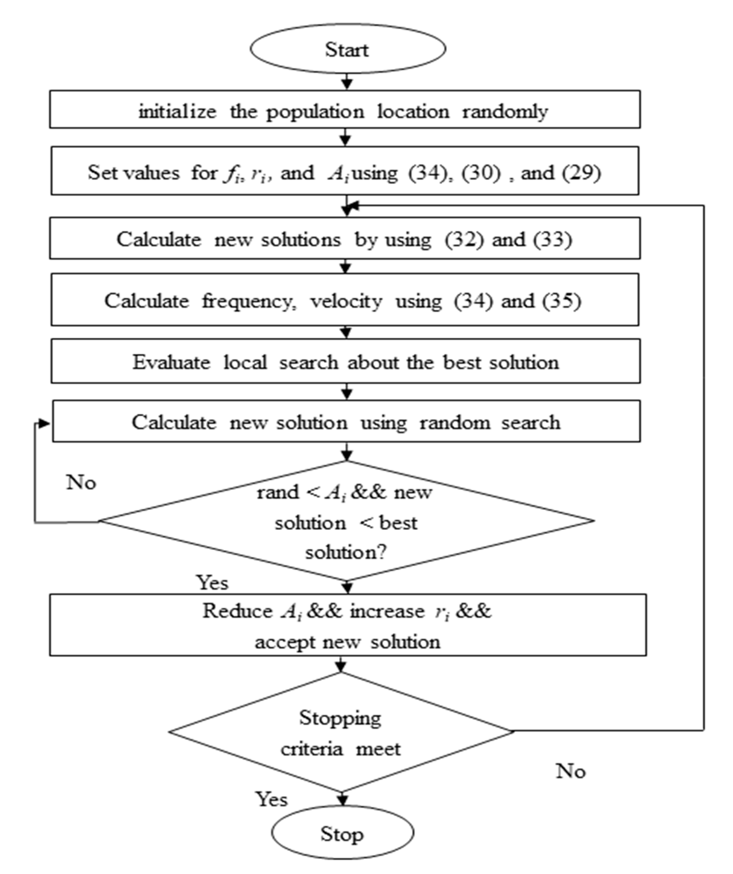
3.2. Quantum-Behaved Bat Algorithm

The basic Bat Algorithm is formulated by using idealized rules. The three rules are, (i) The use of echolocation capability to measure distance and to sense the difference between their prey (food) and background barriers are common to every bat. (ii) If the bats are in $x_i$ position having velocity $v_i$, with $f_{min}$ fixed frequency as well as λ₀ varying wavelength, then loudness A₀ will be used for the search of food while flying randomly. Automated adjustment of the wavelength of their emitted pulses as well as adjustment of the rate of pulses r ϵ [0, 1] can be done by bats which is dependent on target proximity, (iii) It is presumed that loudness changes from a positive large value A₀ to a minimum value A_min that is constant.

Assuming that the solution is not known, to initialize bats randomly, in the search space of each dimension both lower and upper bound is used. The common solution will be generated by using:

$$X_{ij}=X_0-(X_m{X}_0)rand.$$

(24)

For ith bat in the jth dimension $X_0$ and $X_m$ denotes the lower and upper bound, respectively. Considering this, frequency, velocity, and position of bats can be formulated in the following manner:

$$f_i=f_{min}+\left(f_{max}-f_{min}\right)\alpha ;$$

(25)

$$v_i^t=v_i^{t-1}+\left(x_i^t-g^t\right)f_i;$$

(26)

$$x_i^t=x_i^{t-1}+v_i^t$$

(27)

where $\alpha$ is random vector ranging [0, 1]; $f_i$, $f_{min}$ as well as $f_{max}$ are pulse frequency, minimum frequency, and maximum frequency, respectively. Moreover, $v_i^t$, $v_i^{t-1}$, $x_i^t$, $x_i^{t-1},$and $g^t$ denote ith bat’s velocity for t iteration, ith bat’s velocity at (t − 1) iteration, ith bat’s position at t iteration, ith bat’s position at (t − 1) iteration, and global best location currently found by bats, respectively.

For the generation of new solutions for every bat, a random natured local walk is used once a suitable solution is selected from the recent best solutions. Hence, a new position may be expressed as follows:

$$x_n=x_o+\epsilon A^t,$$

(28)

where ε is denoted for expressing a random number ranging [−1, 1] and $A^t$ expresses average loudness of all the bats for total t iterations.

Loudness A_i and pulse rate denoted by r_i are the parameters that control the flow of the bat algorithm. For every iteration, loudness A_i and pulse rate r_i can be found using the following expression:

$$A_i^{t+1}=\mathsf{∆}{A}_i^t,$$

(29)

$$r_i^{t+1}=r_i^0\left[1-\exp (-\gamma t\right)],$$

(30)

where $A_i^t$, $A_i^{t+1}$, $r_i^0$ and $r_i^{t+1}$ denoted for ith bat’s loudness for tth iteration, ith bat’s loudness for (t + 1)th iteration, ith bat’s initial pulse rate, and ith bat’s pulse rate for (t + 1)th iteration, respectively. Both $\mathsf{∆}$ and γ are values that are constant ranging [0, 1] and positive, respectively.

The Quantum-behaved bat algorithm (QBA) is the improved variant of the original bat algorithm. Pioneered in 2010 by Xin-she Yang [49], the original bat algorithm was based on the echolocation or bio-sonar capability of bats. The flowchart of QBA is depicted in Figure 3. The flowchart in Figure 3 shows that after random initialization loudness, frequency and plus rate are updated. After that, the search equation is employed to update search location. A local search is incorporated into the search technique. This process will continue unless the termination criteria are satisfied.

Unlike the traditional bat algorithm, for QBA, a new position is assessed differently, and it can be expressed by the equations below:

$$x_{id}^{t+1}=g_d^t.\left[1+j\left(0,{\sigma }^2\right)\right]{\sigma }^2=\left|A_i^t-A^t\right|+\epsilon ,$$

(31)

where $j\left(0,{\sigma }^2\right)$ denotes a Gaussian distribution that has zero mean and standard deviation of${\sigma }^2$. $x_{id}^{t+1}$ and $g_d^t$ are global best position in d dimension for ith bat’s at t + 1 iteration. $A_i^t$ is ith bat’s loudness for tth iteration. To make sure that the standard deviation ${\sigma }^2$ always remains positive, ε is introduced.

The global best $g_d^t$ in the swarm of bats can be treated as attractor using the Equation (23) and replacing $q_{id}$ by $g_d^t$. The position of the bat with quantum behavior can be expressed by the following equation:

$$x_{id}^t=g_d^t+\beta \left|mbes{t}_d-x_{id}^t\right|\ln (\frac{1}{u}),u\left(0,1\right)<0.5;$$

(32)

$$x_{id}^t=g_d^t-\beta \left|mbes{t}_d-x_{id}^t\right|\ln (\frac{1}{u}),u\left(0,1\right)\ge 0.5;$$

(33)

where $x_{id}^t$ is the ith bat’s position when it is in d dimension for tth iteration. By taking into consideration every bat’s compensation, capability for Doppler Effect that is self-adaptive in nature reforms the updating formulas as per the following expression (23) and (24).

It should be mentioned that for updating the value of velocity as well as for controlling the inheriting rate of the previous velocity, the inertia weight parameter (w) should be added. The compensation rate C should be varied for each bat. Since the velocity of the sound through the normal air is assumed as 340 m/s the expression could be reformed as follows:

$$f_{id}=\frac{\left(340+v_i^{t-1}\right)}{\left(340+v_g^{t-1}\right)}\times f_{id}\times \left[1+C_i\times \frac{\left(g_d^t-x_{id}^t\right)}{\left|g_d^t-x_{id}^t\right|+\epsilon }\right],$$

(34)

$$v_{id}^t=\left(w\times v_{id}^{t-1}\right)+\left(g_d^t-x_{id}^t\right)f_{id},$$

(35)

$$x_{id}^t=x_{id}^{t-1}+v_{id}^t,$$

(36)

where $f_{id}$ is used to denote ith bat’s frequency at dimension d; $v_g^{t-1}$ is denoted for (t − 1)th iteration of the globally best position’s the velocity and $C_i$ is ith bat’s respective positive number ranging [0, 1]. To keep the computation simple, we have assumed that C = 0 leads to the fact that bats will not be able to compensate for Doppler effect in echoes but in the case of C = 1, the bat will be fully capable for compensating Doppler effect in the echoes.

3.3. Advantage and Disadvantage

From No Free Lunch theorem (NFL) it is known that no single algorithm can be best for all problems [50]. After analyzing the major attributes of QBA and QPSO algorithm, three key points for its success can be underscored in the following:

• Better performance can be obtained from quantum-behaved algorithms compared to PSO, GA, CSA, GSA, and DE to carry out highly nonlinear, multi-modal optimization problem as quantum-behaved algorithms has the inherent capability to increase diversity in its population.
• As PSO and GA update their location depending not only on personal best information but also on explicit global best, premature convergence is common in theses algorithms and to avoid this, mean best is used in this algorithm.

According to the No Free Lunch theorem (NFL), a single algorithm cannot be the best solution for every problem [50].

Table 1. Advantages and disadvantages of discussed techniques.

Techniques	Advantage	Disadvantage
GA	Easy to incorporate discrete decision variables. Initializing itself from possible solutions. Higher NPV is achieved than GA	Tuning the algorithm is hard. The convergence and stability linked with the crossover and mutation rates. Less efficient than PSO.
PSO	Less parameter to tune. Simple structure and less dependent on initial points. Incorporating the discrete variable is easy.	Trapped in local optima due to weak local search. A high standard deviation and low efficiency are observed.
DE	DE provides better local search Good balance between exploration and exploitation.	Grater variance in Net present value.
CSA	One parameter needs to be tuned.	Unable to avoid local optima.
BA	Fast convergence.	Unable to avoid local optima.
GSA	High Exploitation rate.	Unable to avoid local optima
QBA	Low Standard deviation is observed Better local search. Standard deviation, efficiency, and effectiveness QBA algorithm is better than the other algorithms.	Computationally expensive. Large number of parameters need to be tuned. Extensive local search causes higher number of function evaluation.
QPSO	Faster convergence and better solution.	Computationally expensive

delineates the overall advantage and disadvantages of these algorithms in brief.

4. Results and Discussion

4.1. Experimental Setting

To validate the proposed methods that are discussed previously, 2 case studies are conducted. Each algorithm ran 16 times. In case study 1, we have used 100 iterations and case study 2 we have used 30 iterations. In case study 1, the search space is 19 × 28 × 5 blocks are present. Again, in case study 2, 10 × 10 × 3 grid blocks are present. Hence, in case study 1, the search space is larger than case study 2. So, algorithms will require more effort to find optimum value in case study one. For PUNQ S3 reservoir 100 iterations is used in the following paper [51]. The detailed description of test case studies are shown in Figure 4 and Figure 5. Again, Figure 6b shows that in case study 2, after a certain iteration the algorithms have reached their optimal result and did not improve further. Furthermore, after a certain point, the curve shows a flat line. The flat line in Figure 6b proves that the algorithms have converged and will not improve further. Hence, 30 iteration is sufficient for case study 2. In each trial, for case study 1, 100 iterations are conducted with 20 particles. A total of 2000 function evaluations are considered as a stopping criterion. In each trial, for case study 2, 30 iterations are conducted with 5 particles. A total of 150 function evaluations are considered as a stopping criterion. The parameters that were used in these algorithms and the economic parameters that were used in Equation (11) to conduct the experiment are listed in

Table 2. Parameters used for metaheuristic algorithms on well placement optimization.

	Literature	Years	Algorithm	Parameter Configuration
1.	[20]	2018	GA	Crossover = 60% Mutation = 5%
2.	[52]	2018	PSO	Inertial factor = 0.729 $c_1$ and $c_2$= 1.494 (Here $c_1$ and $c_2$ represents acceleration)
3.	Proposed	-	QBA	The maximum and minimum inertia weight (wmax and wmin) 0.9 and 0.5 The maximal and minimal frequency (fmax and fmin) 1.5 and 0 Gamma, γ 0.9 Delta, δ 0.99 The frequency of updating the loudness and emission pulse rate, G 10 The maximum and minimum contraction expansion coefficient (βmax and βmin) 1 and 0.5 The maximal and minimal loudness 2 and 1 The maximal and minimal pulse rate 1 and 0 The maximum and minimum compensation rate for Doppler effect (Cmax and Cmin) 1 and 0.9 The maximum and minimum probability of habitat selection 0.9 and 0.6
4.	Proposed	-	QPSO	Maximum number of steps 100 $c_1$ and $c_2$ = 1.494 Initial inertia weight, wmax 1 Final inertia weight, wmin 0.5
5	[53]	2009	GSA	Alfa = 20; G0 = 100;
6	[54,55]	2018	DE	crossover probability, Cr = 0.9 weighting factor F = 0.5
7	[56]	2010	CSA	Flight length, fl = 2 Awareness Probability, Ap = 0.3
8	[57]	2017	BA	Pulse rate = Loudness are = 0.5 Frequency range is [0, 1]

and

Table 3. Economic parameters used by authors in well placement optimization.

Economic Parameter	Value	Unit
Discount rate	10%	-
Oil production cost	72.327	$/STB
Gas price, $P_g$	0.126	$/MScf
Oil price, $P_O$	290.572	$/STB
CAPEX	6.4 × 107	$
Water production cost	31.447	$/STB
Gas price, $P_g$	0.126	$/MScf

.

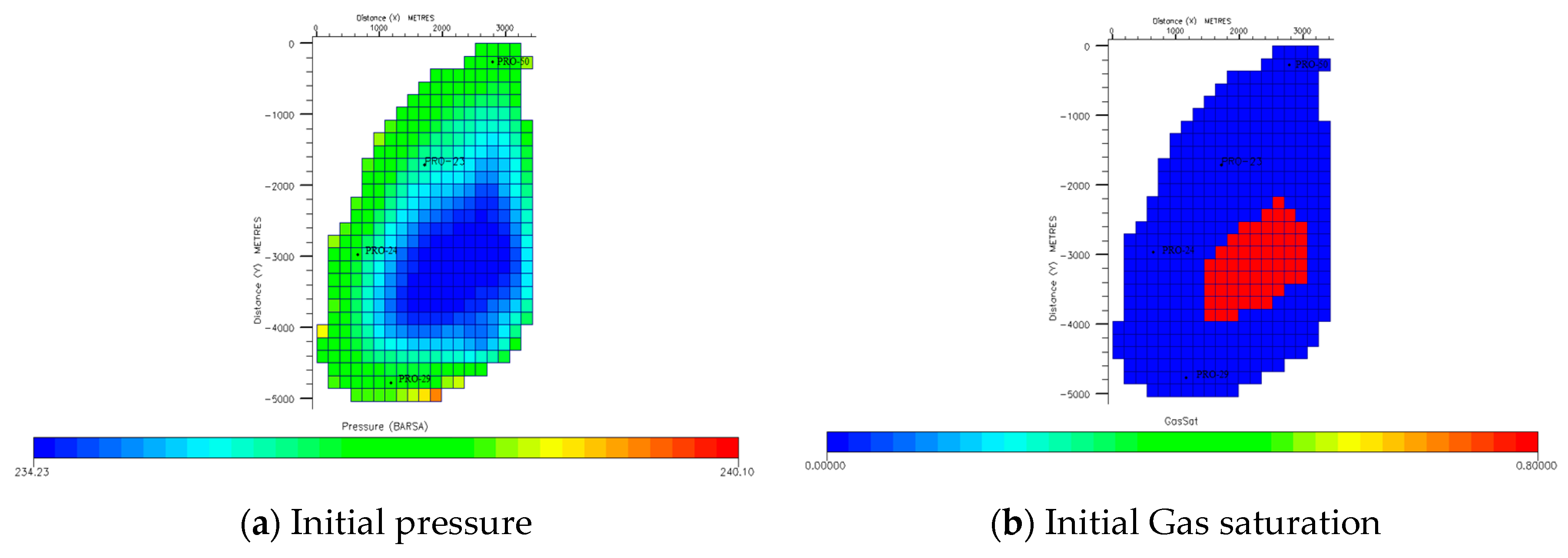
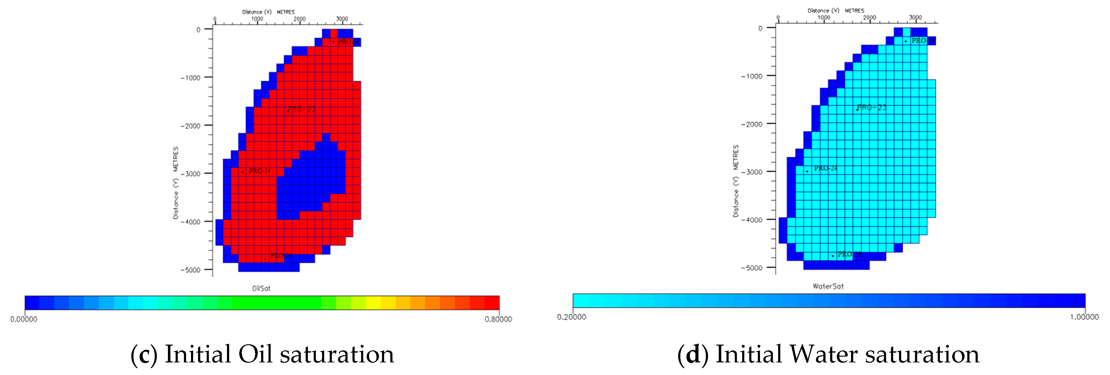
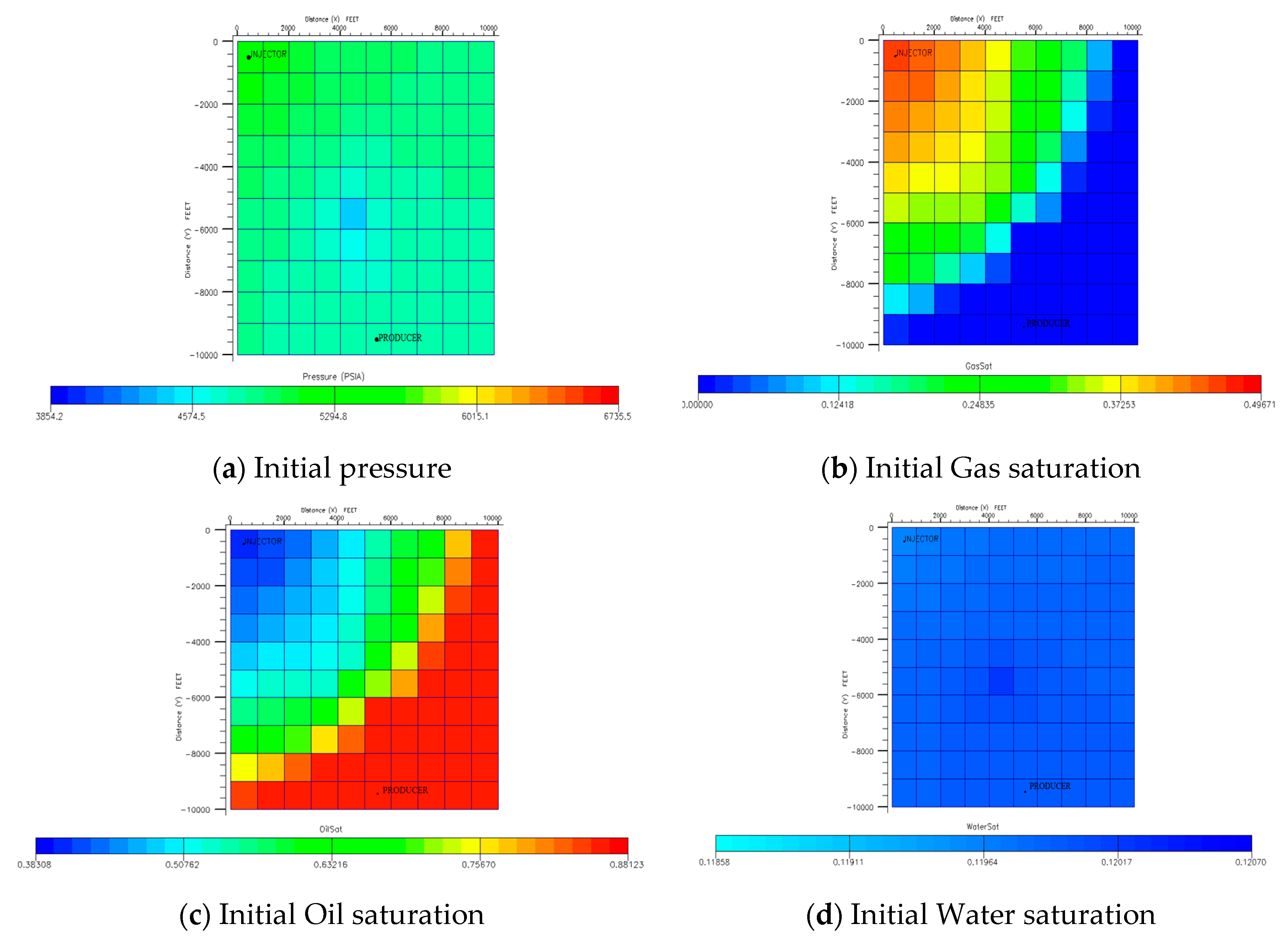
4.2. Description of Case Studies

To select the test cases, the reservoirs that are not identical are considered. The surface of the reservoir can be highly non-smooth or it can multimodal for well placement optimization problem. The PUNQ S3 reservoir can be highly multimodal [26]. So, it will test capacity to tackle the multimodal optimization problem. Again, SPE-1 is fairly simple. So, the case studies will test the capacity to tackle highly multimodal optimization problem and simple multimodal optimization problem.

PUNQ-S3 is a real field-based model and had been used for Elf Exploration production. The detailed characteristics of this reservoir model are analyzed in the literature [58] and shown in Figure 4. The PUNQ-S3 consists of $19\times 28\times 5$ blocks of the grid. To evaluate the proposed technique, the authors have chosen 4 vertical wells that need to be optimized, where each well has $\left(x,y\right)$ coordinates. Thus, the overall number of the variables that need to be optimized in this experiment is $2\times 4$.

To conduct the second case study, the first SPE model is adopted. The first SPE model is formulated based on a 3D black oil reservoir simulation. Hence, this type of synthetic reservoir model is exploited in this study. The detailed characteristics and specification of this reservoir model are discussed in the literature [59] and shown in Figure 5. There are $10\times 10\times 3$ grid blocks in the First SPE model. Two vertical wells locations are optimized in this case study. Since, each well is defined by (x, y) coordinates, $2\times 2$ variables are optimized in this case study.

4.3. Convergence Analysis

To analyze the performance of different algorithms, the convergence curve and convergence speed is an important tool. So, plots of the mean net present value of algorithms versus iterations number are illustrated in Figure 6. As per the illustration of Figure 6a, QPSO algorithm surpassed all the other algorithms. The QBA provided 2nd best results in case study 1. The 3rd and 4th best net present values are achieved by the DE and PSO algorithm, respectively. However, it should be mentioned that both GA, GSA, BA, and CSA have suffered the problem to converge in local optimum point. Overall, in the first case study, QPSO and QBA have achieved better solutions. As seen from Figure 6b, QBA has exhibited superior performance to provide a better net present value compared to other algorithms in case study 2. After QBA, QPSO and PSO algorithms have gained better results than other methods. However, unlike the previous case study, GA performed the worst with respect average net present value. Furthermore, the CSA, GA, BA, and GSA algorithms again failed to obtain satisfactory NPV in this study.

Figure 6 suggests that, unlike PSO and BA algorithm, modification in the search expression in PSO and BA with quantum computation helped avoid local optimum in convergence. Furthermore, the quantum computation in the PSO and BA made it more vibrant across both case studies. Hence, in a multimodal problem, QPSO and QBA is more dynamic than PSO and BA and is further validated by the exploration and exploitation graphs shown in Figure 6.

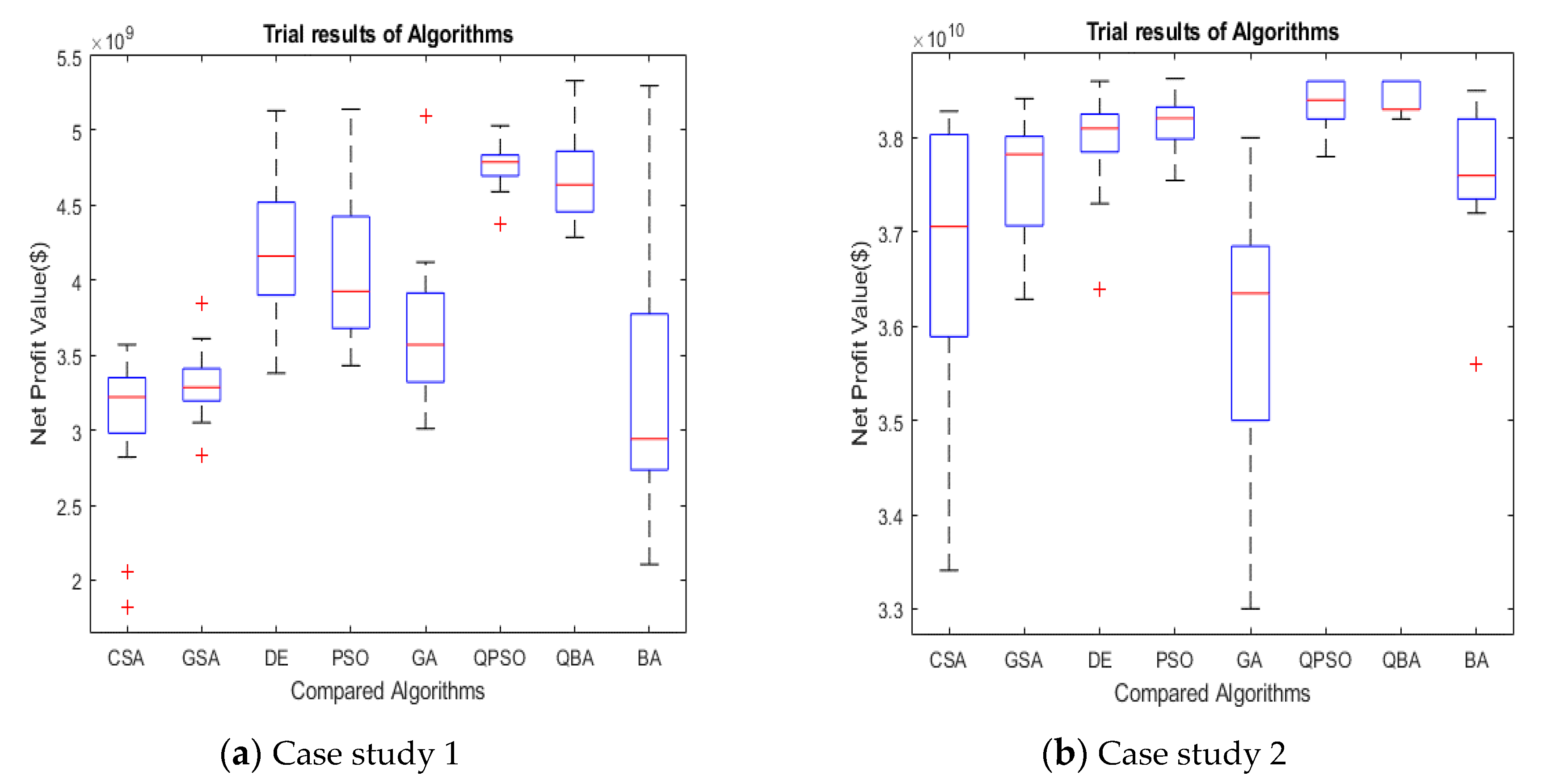
4.4. Performance Evaluation and Statistical Analysis

To assess the discussed algorithms performance, several benchmark criteria are considered for this problem [6,60]. Thus, the author’s preferred benchmark for the evaluation are discussed in the following subsection:

Effectiveness is the average value that is in between consecutive tests where the best solution is expressed with respect to the global optima as a percentage is effective and it is simply a measure of performance. Mathematically, effectiveness can be defined as follows:

$$\overline{f}=\frac{1}{N}{{\displaystyle \sum }}_{i=1}^N\frac{f\left(p_i^{^}\right)}{f\left(p*\right)}$$

(37)

where f(p) is defined as a solution for p, $p*$ is denoted for the solution for global optima, $p_i^{^}$ is referred to as the best solution for ith trial, and N is trial number for each algorithm.

Efficiency is the parameter that is an indicator of the algorithm’s speed at which it reached a specific performance level using a number of distinctive evaluations to obtain a solution that is at least 98 percent of the best value in the experiment.

$$\overline{L}=\frac{1}{N}{\displaystyle \sum }_{i=1}^N\frac{L_i^{98}}{M},$$

(38)

where additionally, $L_i^{98}$ is the number of unique function evaluations required to find solution q such that f(q) _ 0:98f(^pi) for trial i (for minimization) and M is the total number of function evaluations per trial.

Besides these two criteria, statistical data like standard deviation, average, and min-max are collected in experimental trials and the results are shown in

Table 4. Statistical data of applied metaheuristic algorithms on well placement optimization for case study 1.

	GSA	PSO	CSA	GA	DE	BA	QPSO	QBA
Max	3.84 × 109	5.14 × 109	3.72 × 109	5.09 × 109	5.13 × 109	5.30 × 109	5.03 × 109	5.33 × 109
Min	2.83 × 109	3.43 × 109	2.43 × 109	3.01 × 109	3.38 × 109	2.10 × 109	4.38 × 109	4.29 × 109
Average	3.33 × 109	4.07 × 109	3.24 × 109	3.67 × 109	4.26 × 109	3.28 × 109	4.77 × 109	4.67 × 109
Standard deviation	2.62 × 108	5.72 × 108	3.73 × 108	5.11 × 108	4.59 × 108	8.35 × 108	1.60 × 108	2.74 × 108
Effectiveness	6.24 × 10−1	7.63 × 10−1	6.08× 10−1	6.88 × 10−1	8.00 × 10−1	6.16 × 10−1	8.94 × 10−1	8.76 × 10−1
Efficiency	1.39 × 10−1	5.53 × 10−1	5.09 × 10−1	4.78 × 10−1	6.46 × 10−1	8.25 × 10−1	4.28 × 10−1	5.38 × 10−1

and

Table 5. Statistical data of applied metaheuristic algorithms on well placement optimization for case study 2.

	GSA	PSO	CSA	GA	DE	BA	QPSO	QBA
Max	3.84 × 1010	3.86 × 1010	3.83 × 1010	3.80 × 1010	3.86 × 1010	3.85 × 1010	3.86 × 1010	3.86 × 1010
Min	3.63 × 1010	3.75 × 1010	3.34 × 1010	3.30 × 1010	3.64 × 1010	3.56 × 1010	3.78 × 1010	3.82 × 1010
Average	3.76 × 1010	3.82 × 1010	3.66 × 1010	3.60 × 1010	3.80 × 1010	3.76 × 1010	3.84 × 1010	3.84 × 1010
Standard deviation	6.21 × 108	3.09 × 108	1.63 × 108	1.37 × 108	5.39 × 108	6.92 × 108	2.58 × 108	1.61 × 108
Effectiveness	9.74 × 10−1	9.89 × 10−1	9.49 × 10−1	9.32 × 10−1	9.84 × 10−1	9.74 × 10−1	9.93 × 10−1	9.95 × 10−1
Efficiency	9.79 × 10−2	1.52 × 10−1	1.54 × 10−1	1.23 × 10−1	1.46 × 10−1	1.00 × 10−1	2.17 × 10−1	1.79 × 10−1

.

The mean value and standard deviation indicate the robustness of the algorithm. The results of Case Study 1 show that the QPSO algorithm is optimal on four criteria. However, QBA was better on 2 other criteria. The box plot results are shown in Figure 7a indicates that QPSO and QBA have reached almost similar results compared to other algorithms and QPSO has the lowest standard deviation.

Again, the result of case study 2 in Table 5 shows that the QPSO and QBA algorithm is superior on three and five criteria, respectively. However, PSO and DE also achieved the same maximum value, their average value is lower than QBA and QPSO. The box plot results in Figure 7b illustrates that QBA has the lowest standard deviation compared to other algorithms, and QPSO has the second-lowest standard deviation. The main results of the study of case 2 are somewhat tantamount to the previous study as it shows quantum-based algorithms are a better choice considering all 6 criteria.

4.5. Wilcoxon’s Rank-Sum Test

To validate whether the results of QPSO and QBA are statistically different from the other six algorithms, a non-parametric statistical test, the Wilcoxon rank-sum test [61,62], with a significance level of 0.05, is used.

Table 6. Statistical data of applied metaheuristic algorithms on well placement optimization for case study 1 reservoir.

	Case Study 1			Case Study 2
	Z Value	p Value One Tail	p Value Two Tails	Z Value	p Value One Tail	p Value Two Tails
QPSO Versus GSA	3.5033	0.00022979	0.00045958	3.3481	0.00040678	0.00081355
QPSO Versus PSO	3.0379	0.0011912	0.0023824	1.6418	0.050321	0.10064
QPSO Versus CSA	3.5033	0.00022979	0.00045958	3.2447	0.00058782	0.0011756
QPSO Versus DE	2.9867	0.0014101	0.0028202	2.1416	0.016113	0.032226
QPSO Versus GA	3.4516	0.00027868	0.00055736	3.5044	0.00022878	0.00045757
QPSO Versus BA	3.3999	0.00033711	0.00067422	3.428	0.00030402	0.00060805
QBA Versus GSA	3.5033	0.00022979	0.00045958	3.3999	0.00033711	0.00067422
QBA Versus PSO	2.9862	0.0014124	0.0028249	2.5216	0.0058404	0.011681
QBA Versus CSA	3.5033	0.00022979	0.00045958	3.5033	0.00022979	0.00045958
QBA Versus DE	2.5725	0.0050482	0.010096	3.0735	0.0010578	0.0021155
QBA Versus GA	3.3481	0.00040678	0.00081355	3.5044	0.00022878	0.00045757
QBA Versus BA	3.2964	0.0004896	0.00097921	3.3245	0.00044287	0.00088574
QBA Versus QPSO	1.3315	0.091512	0.18302	0.74132	0.22925	0.4585

shows the p-value one tail, p-value two tails, and Z values for the Wilcoxon rank sums test. A p-value less than 0.05 and Z value higher than 1.96 is required to reject the null hypothesis. From Table 6 it can be inferred that there is a statistical difference between the performance of QPSO and QBA with other algorithms except in one case. In case study 1 and 2, the performance of the QPSO and QBA are not statistically different. Therefore, it can be inferred that quantum computation can bring improved results from the other six algorithms. However, QPSO and QBA’s proved to be statistically different from its primary algorithm.

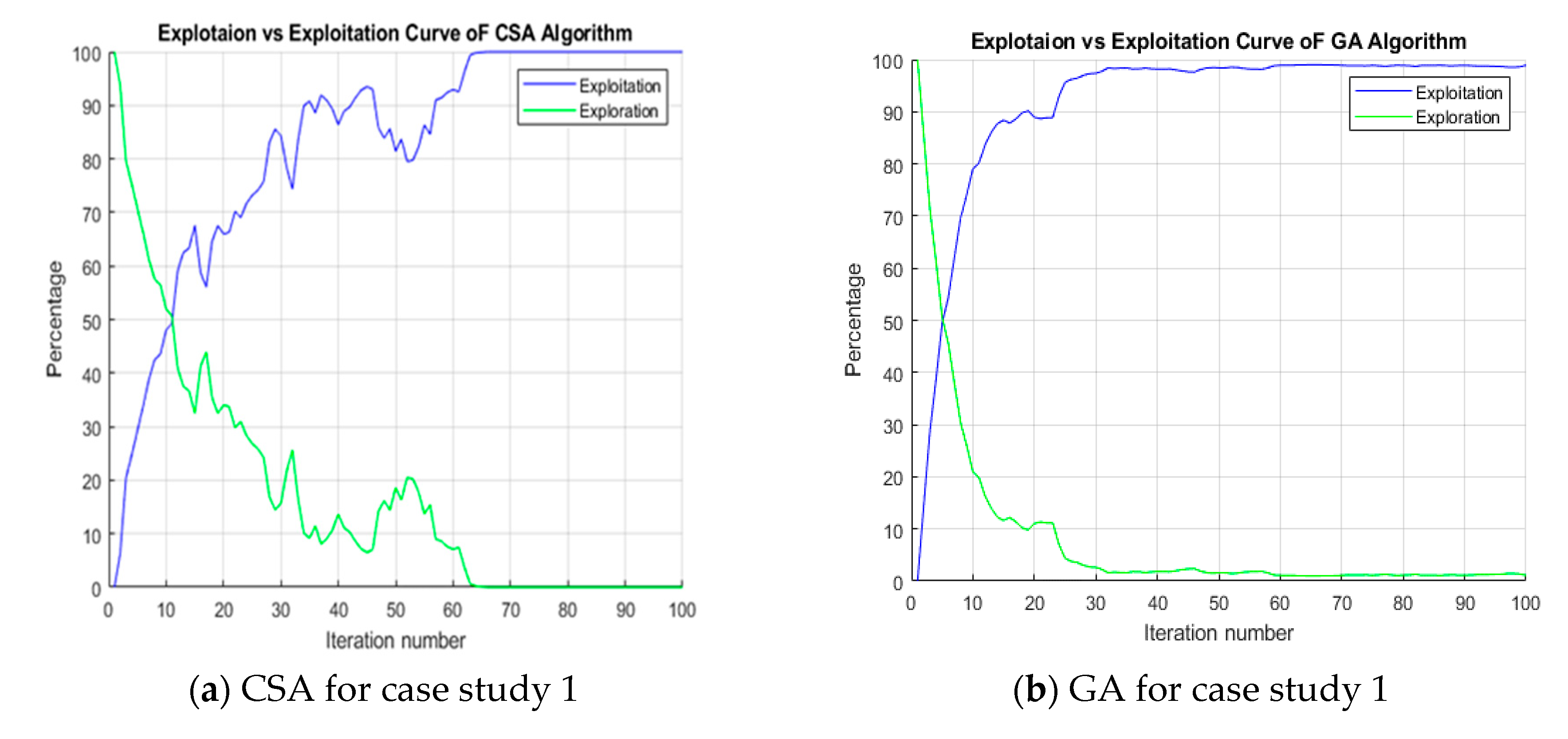
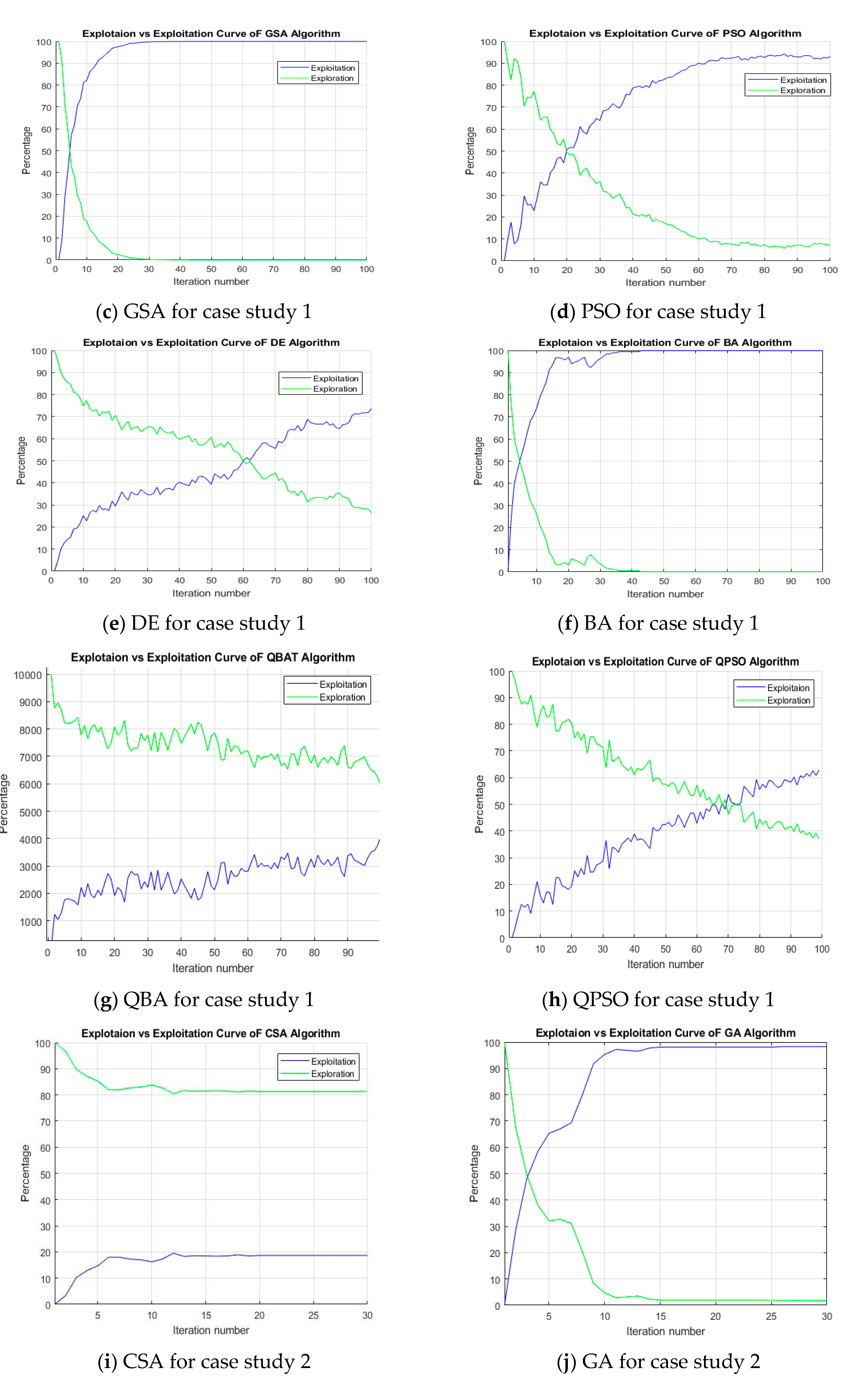
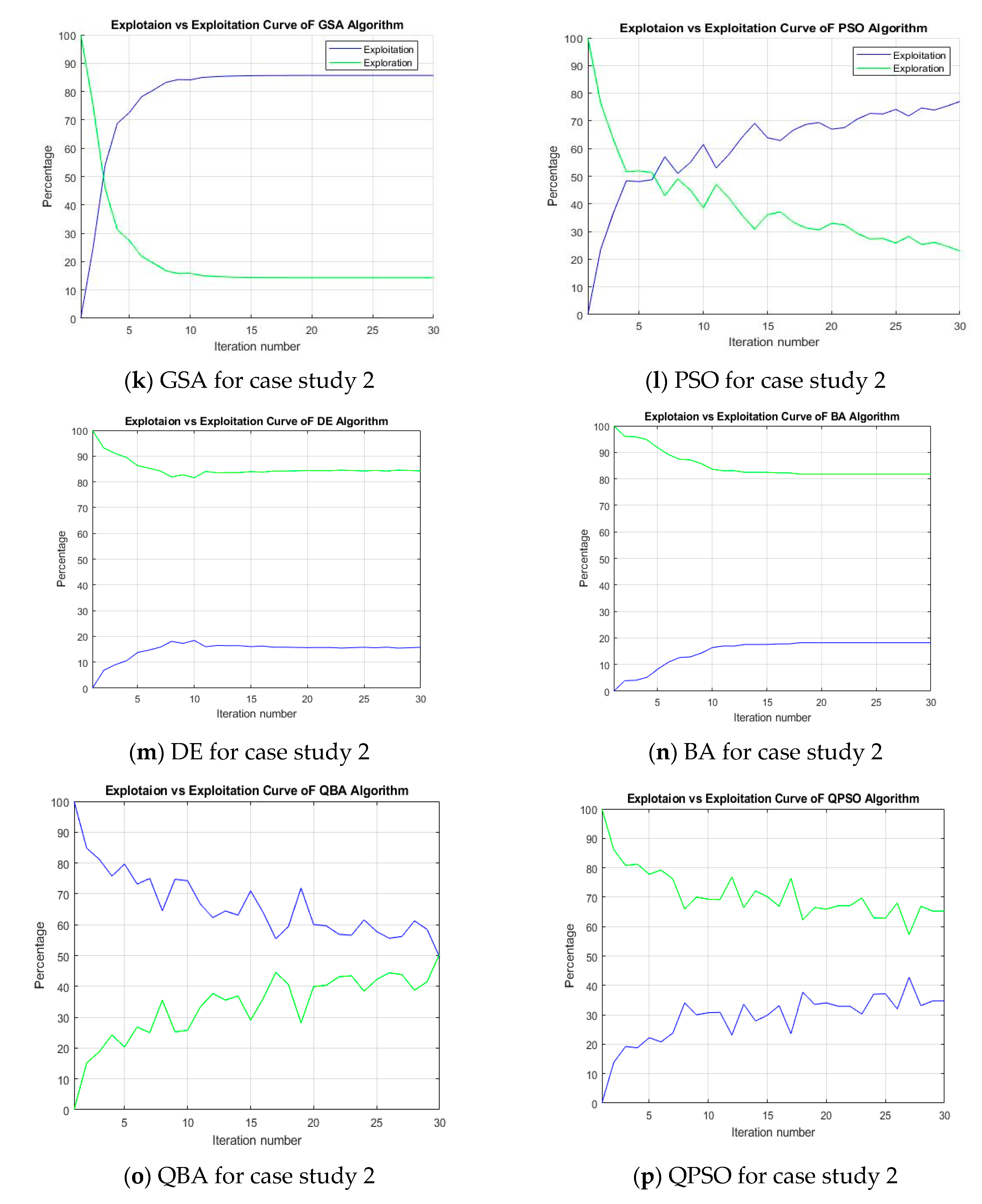
4.6. Exploration and Exploitation Analysis

Dimension wise analysis sheds light on the internal behavior of the algorithms [63]. In this context, it is important to have a strong diversification to better exploit the search space. A small degree of diversification implies local convergence. To measure the diversity in each dimension, the authors have considered the equation proposed in Reference [64]:

$$Di{v}_j=\frac{1}{n}{\displaystyle \sum }_{i=1}^n|median(x_j)-x_{ij}|,$$

(39)

where $x_{ij}$ is the dimension$j$ of the ith swarm, $median(x_j)$ refers to the median of dimension $j$ in the whole population, and n is the total number of the population. So, the average diversity can be calculated using Equation (40):

$$Div=\frac{1}{D}{{\displaystyle \sum }}_{i=1}^{n}Di{v}_j,$$

(40)

where $Div$ is the diversity measurement of the whole population in an iteration.

Hence, Exploration and Exploitation can be measured using the following equation:

$$Exploration=\frac{Div}{Di{v}_{max}}\times 100,$$

(41)

$$Exploitation=(1-\frac{Div}{Di{v}_{max}})\times 100,$$

(42)

where, $Di{v}_{max}$ presents the maximum diversity of whole populations in one run.

Without revealing the behavior of swarms in the iterative process, it is difficult to understand the end result and the value of the objective function. Therefore, to understand the end results of these techniques or convergence curve in Figure 6, this study initiates a graphical illustration to show the algorithms’ exploration and exploitation behavior over the whole iteration. From Figure 8, it can be inferred that a higher NPV can be achieved with an adequate exploration and development ratio. On the other hand, these figures clearly indicate a gradual change in intensity during exploration and exploitation during the iterative process.

The graphs shown in Figure 6 shows that while QPSO and QBA has a high average exploration rate. On the other hand, CSA, GSA, and GA had a relatively low exploration rate. In case Study 1, the overall exploration rate of QBA and QPSO is 74% and 60%, respectively, and a quantum behaved algorithm offered a better optimal solution. Again, among all algorithms, the least average exploration group contains BA, GA, CSA, and GSA and their exploration rate was 6.6%, 8.2%, 17.4%, and 6.4%, respectively. This shows that the average diversity obtained by the other algorithms is much less than the quantum-behaved algorithms. Furthermore, it can be noted that BA, GA, CSA, and GSA obtained the least average NPV value and quantum-behaved algorithms offer a better optimal solution. Again, PSO and DE obtained 27.4% and 54.6% exploration rate, respectively.

On the other hand, in case study 2, the average diversity of BA, CSA, and DE was 85.1%, 83.3%, and 85.2%, respectively. In this case, BA provides the highest exploration rate. However, BA and CSA were unable to achieve better optimization results. Hence, it showcases that the higher exploration rates are not necessary to optimize the well location. Again, PSO, GSA, and GA achieved 39%, 21.93%, 14.2% exploration rates. Moreover, PSO was able to achieve 3rd best average NPV. Similarly, 1st and 2nd best average NPV provider QBA and QPSO achieved 66.4%, 71% exploration, respectively. Therefore, the correct exploration-exploitation ratio should be carefully calculated according to the search field. In general, a roughly balanced response indicates that the algorithm is more efficient. This seems to be one of the explanations for the successful results of The QPSO and QBA algorithm.

Another important finding in this study is the successful search is produced through exploration mechanisms with the effective exploration of mechanisms and appropriate balanced responses. In some cases, the two metaheuristic algorithms offer very different performances to the quality of the solution, but the balanced responses are similar (i.e., in case study 2, DE and BA’s Exploration percentage = 85, exploitation percentage = 15). It simply means that there are not enough balanced solutions to produce successful performance. Therefore, operators must consider the correct diversity conditions in a balanced response to produce viable options.

This study has limitations, as it is primarily focused on optimization methods. Uncertainty quantification and history matching have not been considered. The primary emphasis is on areas such as utilize quantum computation for reservoirs, enhancing efficiency, and increasing the NPV performance of well positioning. The emphasis in this analysis is only on the algorithm for optimization.

5. Conclusions

In this study, quantum computation is implemented for well placement optimization and their application to well placement optimization problem is investigated. Experimental results suggested that the QBA and QPSO algorithm can find a better solution than popular algorithms. It is true that due to strong attraction to local attractor QBA has a strong local search capacity that helped it to tackle this multimodal problem more efficiently. It can be inferred that quantum computation can bring improved results compared to other six algorithms. This study showcases that higher exploration rates are not necessary to optimize the well location. However, the correct exploration-exploitation ratio is should be carefully calculated in the task area. In general, a roughly balanced response indicates that the algorithm is more efficient. This seems to be one of the explanations for the successful results of The QPSO and QBA algorithm. The main conclusions of this paper are as follows:

No global search algorithm can perform well on all kinds of reservoirs. Different reservoir requires different strategy.

Quantum techniques increase exploration rate in the search technique, which helps to find better results.

There is no statistical difference in the results of QBA and QPSO.

The particles are volatile and diverse owning to the local attractor points.

Quantum techniques are less susceptible to premature convergence and less likely to be stuck in local optima.

High exploitation rate can be linked with lower NPV value.

Diversity analysis reveals that dynamic exploration and exploitation strategy is required for each reservoir.

Future optimization studies should focus on using the global search algorithm with a local search approach because it may have the advantage of solving well placement optimization problem successfully. Lots of research papers have used proxy models in recent years to replace actual reservoir simulators, and these models have been found to minimize runtime. The accuracy of this alternative model, therefore, depends on its range of sampling. Future research in this area may focus on improving the reliability of this technique.

References

1. Rosenwald, G.W.; Green, D.W. A method for determining the optimum location of wells in a reservoir using mixed-integer programming. Soc. Pet. Eng. J. 1974, 14, 44–54. [Google Scholar] [CrossRef]
2. Ma, X.; Plaksina, T.; Gildin, E. Integrated horizontal well placement and hydraulic fracture stages design optimization in unconventional gas reservoirs. In Proceedings of the SPE/CSUR Unconventional Resources Conference; Society of Petroleum Engineers (SPE), Calgary, AB, Canada, 5–7 November 2013. [Google Scholar]
3. Pan, Y.; Horne, R.N. Improved methods for multivariate optimization of field development scheduling and well placement design. In Proceedings of the SPE Annual Technical Conference and Exhibition, Society of Petroleum Engineers, New Orleans, LA, USA, 27–30 September 1998. [Google Scholar]
4. Li, L.; Jafarpour, B. A variable-control well placement optimization for improved reservoir development. Comput. Geosci. 2012, 16, 871–889. [Google Scholar] [CrossRef]
5. Jansen, J. Adjoint-based optimization of multi-phase flow through porous media—A review. Comput. Fluids 2011, 46, 40–51. [Google Scholar] [CrossRef]
6. Bangerth, W.; Klie, H.; Wheeler, M.F.; Stoffa, P.L.; Sen, M.K. On optimization algorithms for the reservoir oil well placement problem. Comput. Geosci. 2006, 10, 303–319. [Google Scholar] [CrossRef]
7. Zhang, L.; Zhang, K.; Chen, Y.; Li, M.; Yao, J.; Li, L.; Lee, J. Smart Well Pattern Optimization Using Gradient Algorithm. J. Energy Resour. Technol. 2015, 138, 012901. [Google Scholar] [CrossRef]
8. Siavashi, M.; Tehrani, M.R.; Nakhaee, A. Efficient Particle Swarm Optimization of Well Placement to Enhance Oil Recovery Using a Novel Streamline-Based Objective Function. J. Energy Resour. Technol.-Trans. Asme 2016, 138, 052903. [Google Scholar] [CrossRef]
9. Isebor, O.J.; Durlofsky, L.J.; Ciaurri, D.E. A derivative-free methodology with local and global search for the constrained joint optimization of well locations and controls. Comput. Geosci. 2013, 18, 463–482. [Google Scholar] [CrossRef]
10. Giuliani, C.M.; Camponogara, E. Derivative-free methods applied to daily production optimization of gas-lifted oil fields. Comput. Chem. Eng. 2015, 75, 60–64. [Google Scholar] [CrossRef]
11. Forouzanfar, F.; Reynolds, A. Well-placement optimization using a derivative-free method. J. Pet. Sci. Eng. 2013, 109, 96–116. [Google Scholar] [CrossRef]
12. Davarpanah, A. Feasible analysis of reusing flowback produced water in the operational performances of oil reservoirs. Environ. Sci. Pollut. Res. 2018, 25, 35387–35395. [Google Scholar] [CrossRef]
13. Davarpanah, A.; Nassabeh, S.M.M.; Mirshekari, B. Optimization of drilling parameters by analysis of formation strength properties with utilization of mechanical specific energy. Open J. Geol. 2017, 7, 1590–1602. [Google Scholar] [CrossRef] [Green Version]
14. Chang, C.; Li, Y.; Li, X.; Liu, C.; Fiallos-Torres, M.; Yu, W. Effect of complex natural fractures on economic well spacing optimization in shale gas reservoir with gas-water two-phase flow. Energies 2020, 13, 2853. [Google Scholar] [CrossRef]
15. Zhu, M.; Yu, L.; Zhang, X.; Davarpanah, A. Application of implicit pressure-explicit saturation method to predict filtrated mud saturation impact on the hydrocarbon reservoirs formation damage. Mathematics 2020, 8, 1057. [Google Scholar] [CrossRef]
16. Sun, S.; Zhou, M.; Lu, W.; Davarpanah, A. Application of symmetry law in numerical modeling of hydraulic fracturing by finite element method. Symmetry 2020, 12, 1122. [Google Scholar] [CrossRef]
17. Davarpanah, A.; Mirshekari, B. Mathematical modeling of injectivity damage with oil droplets in the waste produced water re-injection of the linear flow. Eur. Phys. J. Plus 2019, 134, 180. [Google Scholar] [CrossRef]
18. Khoshneshin, R.; Sadeghnejad, S. Integrated well placement and completion optimization using heuristic algorithms: A case study of an iranian carbonate formation. J. Chem. Pet. Eng. 2018, 52, 35–47. [Google Scholar]
19. Afshari, S.; Aminshahidy, B.; Pishvaie, M.R. Application of an improved harmony search algorithm in well placement optimization using streamline simulation. J. Pet. Sci. Eng. 2011, 78, 664–678. [Google Scholar] [CrossRef]
20. Túpac, Y.J.; Vellasco, M.M.R.; Pacheco, M.A.C. Planejamento e otimização do desenvolvimento de um campo de petróleo por algoritmos genéticos. In Proceedings of the VIII International Conference on Industrial Engineering and Operations Management, Bandung, Indonesia, 23–25 October 2002. [Google Scholar]
21. Montes, G.; Bartolome, P.; Udias, A.L. The use of genetic algorithms in well placement optimization. In Proceedings of the SPE Latin American and Caribbean Petroleum Engineering Conference, Bueanos Aires, Argentina, 25–28 March 2001; Society of Petroleum Engineers: Richardson, TX, USA, 2001. [Google Scholar]
22. Yeten, B.; Durlofsky, L.J.; Aziz, K. Optimization of nonconventional well type, location, and trajectory. SPE J. 2003, 8, 200–210. [Google Scholar] [CrossRef]
23. Güyagüler, B.; Horne, R.N. Uncertainty assessment of well-placement optimization. SPE Reserv. Eval. Eng. 2004, 7, 24–32. [Google Scholar] [CrossRef]
24. Lyons, J.; Nasrabadi, H. Well placement optimization under time-dependent uncertainty using an ensemble Kalman filter and a genetic algorithm. J. Pet. Sci. Eng. 2013, 109, 70–79. [Google Scholar] [CrossRef]
25. Feng, Q.; Chen, H.; Wang, X.; Wang, S.; Wang, Z.; Yang, Y.; Bing, S. Well control optimization considering formation damage caused by suspended particles in injected water. J. Nat. Gas Sci. Eng. 2016, 35, 21–32. [Google Scholar] [CrossRef]
26. Awotunde, A.A. Inclusion of well schedule and project life in Well Placement Optimization. In Proceedings of the Nigeria Annual International Conference and Exhibition; Society of Petroleum Engineers (SPE), Lagos, Nigeia, 5–7 August 2014. [Google Scholar]
27. Alghareeb, Z.M.; Walton, S.P.; Williams, J.R. Well Placement optimization under constraints using modified cuckoo search. In Proceedings of the SPE Saudi Arabia Section Technical Symposium and Exhibition; Society of Petroleum Engineers (SPE), Al-Khobar, Saudi Arabia, 21–24 April 2014. [Google Scholar]
28. Naderi, M.; Khamehchi, E. Application of DOE and metaheuristic bat algorithm for well placement and individual well controls optimization. J. Nat. Gas Sci. Eng. 2017, 46, 47–58. [Google Scholar] [CrossRef]
29. Ma, J.; Di, P.; Shen, Y.; Liang, Y.; Zhang, H.; Huang, A.; Huang, Z. An intelligent method for deep-water injection-production well pattern design. In Proceedings of the 28th International Ocean and Polar Engineering Conference: International Society of Offshore and Polar Engineers, Sapporo, Japan, 10–15 June 2018. [Google Scholar]
30. Al Dossary, M.A.; Nasrabadi, H. Well placement optimization using imperialist competitive algorithm. J. Pet. Sci. Eng. 2016, 147, 237–248. [Google Scholar] [CrossRef] [Green Version]
31. Humphries, T.D.; Haynes, R.; James, L. Simultaneous and sequential approaches to joint optimization of well placement and control. Comput. Geosci. 2013, 18, 433–448. [Google Scholar] [CrossRef]
32. Aliyev, E. Use of Hybrid Approaches and Metaoptimization for Well Placement Problems. Ph.D. Thesis, Stanford University, Stanford, CA, USA, 2011. [Google Scholar]
33. Emerick, A.A.; Silva, E.; Messer, B.; Almeida, L.F.; Szwarcman, D.; Pacheco, M.A.C.; Vellasco, M.M.B.R. Well placement optimization using a genetic algorithm with nonlinear constraints. SPE Reserv. Simul. Symp. 2009. [Google Scholar] [CrossRef]
34. Negash, B.M.; Yaw, A.D. Artificial neural network based production forecasting for a hydrocarbon reservoir under water injection. Pet. Explor. Dev. 2020, 47, 383–392. [Google Scholar] [CrossRef]
35. Siddiqui, M.A.Q.; Khan, R.A.; Jamal, S. Multi-objective well placement optimization considering energy sustainability along with economical gains. In Proceedings of the SPE North Africa Technical Conference and Exhibition, Society of Petroleum Engineers (SPE), Cairo, Egypt, 14–16 September 2015. [Google Scholar]
36. Hamida, Z.; Azizi, F.; Saad, G.A. An efficient geometry-based optimization approach for well placement in oil fields. J. Pet. Sci. Eng. 2017, 149, 383–392. [Google Scholar] [CrossRef]
37. Nwankwor, E.; Nagar, A.K.; Reid, D.C. Hybrid differential evolution and particle swarm optimization for optimal well placement. Comput. Geosci. 2012, 17, 249–268. [Google Scholar] [CrossRef]
38. Onwunalu, J.E.; Durlofsky, L.J. Application of a particle swarm optimization algorithm for determining optimum well location and type. Comput. Geosci. 2009, 14, 183–198. [Google Scholar] [CrossRef]
39. Negash, B.M.; Ayoub, M.A.; Jufar, S.R.; Robert, A.J. History matching using proxy modeling and multiobjective optimizations. In ICIPEG 2016; Springer Science and Business Media LLC: Berlin/Heidelberg, Germany, 2017; pp. 3–16. [Google Scholar]
40. Negash, B.M.; Him, P.C. Reconstruction of missing gas, oil, and water flow-rate data: A unified physics and data-based approach. SPE Reserv. Eval. Eng. 2020. [Google Scholar] [CrossRef]
41. Abukhamsin, A.Y.J.U.M.t. Optimization of Well Design and Location in a Real Field; Stanford University: Stanford, CA, USA, 2009. [Google Scholar]
42. Aziz, K.; Settari, A. Petroleum Reservoir Simulation; Applied Science Publ. Ltd.: London, UK, 1979. [Google Scholar]
43. Ross, O.H.M. A Review of Quantum-Inspired Metaheuristics: Going from Classical Computers to Real Quantum Computers; IEEE Access: Piscataway, NJ, USA, 2019. [Google Scholar]
44. Karmakar, S.; Dey, A.; Saha, I. Use of quantum-inspired metaheuristics during last two decades. In Proceedings of the 2017 7th International Conference on Communication Systems and Network Technologies (CSNT), Nagpur, India, 11–13 November 2017; Institute of Electrical and Electronics Engineers (IEEE): Piscataway, NJ, USA, 2017; pp. 272–278. [Google Scholar]
45. Jamasb, A.; Motavalli-Anbaran, S.-H.; Zeyen, H. Non-linear stochastic inversion of gravity data via quantum-behaved particle swarm optimisation: Application to Eurasia-Arabia collision zone (Zagros, Iran). Geophys. Prospect. 2017, 65, 274–294. [Google Scholar] [CrossRef]
46. Zhu, B.; Zhu, W.; Liu, Z.; Duan, Q.; Cao, L. A Novel Quantum-Behaved Bat Algorithm with Mean Best Position Directed for Numerical Optimization. Comput. Intell. Neurosci. 2016, 2016, 1–17. [Google Scholar] [CrossRef] [PubMed] [Green Version]
47. Poli, R.; Kennedy, J.; Blackwell, T. Particle swarm optimization. Swarm Intell. 2007, 1, 33–57. [Google Scholar] [CrossRef]
48. Sun, J.; Feng, B.; Xu, W. Particle swarm optimization with particles having quantum behavior. In Proceedings of the 2004 Congress on Evolutionary Computation (IEEE Cat No 04TH8753) CEC-04, Portland, OR, USA, 19–23 June 2004; Institute of Electrical and Electronics Engineers (IEEE): Piscataway, NJ, USA, 2004. [Google Scholar]
49. Yumin, D.; Li, Z. Quantum behaved particle swarm optimization algorithm based on artificial fish swarm. Math. Probl. Eng. 2014, 2014, 1–10. [Google Scholar] [CrossRef]
50. Meng, K.; Wang, H.-G.; Dong, Z.; Wong, K.P. Quantum-inspired particle swarm optimization for valve-point economic load dispatch. IEEE Trans. Power Syst. 2009, 25, 215–222. [Google Scholar] [CrossRef]
51. Sun, J.; Fang, W.; Wu, X.; Palade, V.; Xu, W. Quantum-behaved particle swarm optimization: Analysis of individual particle behavior and parameter selection. Evol. Comput. 2012, 20, 349–393. [Google Scholar] [CrossRef]
52. Sun, J.; Xu, W.; Liu, J. Parameter selection of quantum-behaved particle swarm optimization. In Proceedings of the Computer Vision, San Diego, CA, USA, 20–25 June 2005; Springer Science and Business media LLC: Berlin/Heidelberg, Germany, 2005; Volume 3612, pp. 543–552. [Google Scholar]
53. Yang, X.-S. A New Metaheuristic Bat-Inspired Algorithm. In Advanced Approaches to Intelligent Information and Database Systems; Springer Science and Business Media LLC: Berlin/Heidelberg, Germany, 2010; Volume 284, pp. 65–74. [Google Scholar]
54. Wolpert, D.; Macready, W. No free lunch theorems for optimization. IEEE Trans. Evol. Comput. 1997, 1, 67–82. [Google Scholar] [CrossRef] [Green Version]
55. Boah, E.A.; Kondo, O.K.S.; Borsah, A.A.; Brantson, E.T. Critical evaluation of infill well placement and optimization of well spacing using the particle swarm algorithm. J. Pet. Explor. Prod. Technol. 2019, 9, 3113–3133. [Google Scholar] [CrossRef] [Green Version]
56. Khan, R.A.; Awotunde, A.A. Determination of vertical/horizontal well type from generalized field development optimization. J. Pet. Sci. Eng. 2018, 162, 652–665. [Google Scholar] [CrossRef]
57. Rashedi, E.; Nezamabadi-Pour, H.; Saryazdi, S. GSA: A gravitational search algorithm. Inf. Sci. 2009, 179, 2232–2248. [Google Scholar] [CrossRef]
58. Chen, H.; Feng, Q.; Zhang, X.; Wang, S.; Zhou, W.; Liu, C. Well placement optimization for offshore oilfield based on theil index and differential evolution algorithm. J. Pet. Explor. Prod. Technol. 2017, 8, 1225–1233. [Google Scholar] [CrossRef] [Green Version]
59. Foroud, T.; Baradaran, A.; Seifi, A. A comparative evaluation of global search algorithms in black box optimization of oil production: A case study on Brugge field. J. Pet. Sci. Eng. 2018, 167, 131–151. [Google Scholar] [CrossRef]
60. Askarzadeh, A. A novel metaheuristic method for solving constrained engineering optimization problems: Crow search algorithm. Comput. Struct. 2016, 169, 1–12. [Google Scholar] [CrossRef]
61. Naderi, M.; Khamehchi, E. Well placement optimization using metaheuristic bat algorithm. J. Pet. Sci. Eng. 2017, 150, 348–354. [Google Scholar] [CrossRef]
62. Floris, F.J.T.; Bush, M.D.; Cuypers, M.; Roggero, F.; Syversveen, A.-R. Methods for quantifying the uncertainty of production forecasts: A comparative study. Pet. Geosci. 2001, 7, S87–S96. [Google Scholar] [CrossRef]
63. Minton, J. A Comparison of common methods for optimal well placement. SIAM Undergrad. Res. Online 2014, 7. [Google Scholar] [CrossRef]
64. Clerc, M. From theory to practice in particle swarm optimization. In Adaptation, Learning, and Optimization; Springer Science and Business Media LLC: Berlin/Heidelberg, Germany, 2011; Volume 8, pp. 3–36. [Google Scholar]
Figure 1. A general flow chart for searching the maximum net present value.
Applsci 10 07000 g001
Figure 2. Flowchart of quantum particle swarm optimization (QPSO).
Applsci 10 07000 g002
Figure 3. Flowchart of quantum-behaved bat algorithm (QBA).
Applsci 10 07000 g003
Figure 4. Description for case study 1.
Applsci 10 07000 g004aApplsci 10 07000 g004b
Figure 5. Description for case study 2.
Applsci 10 07000 g005
Figure 6. Convergence curve for PSO, crow search algorithm (CSA), gravitational search algorithm (GSA), and Niching CSA (NCSA) for case study 1 and 2.
Applsci 10 07000 g006
Figure 7. Box plot for PSO, GSA, CSA, and NCSA for case study 1 and case study 2.
Applsci 10 07000 g007
Figure 8. Exploration and exploitation.
Applsci 10 07000 g008aApplsci 10 07000 g008bApplsci 10 07000 g008c