Compression of Vehicle Trajectories with a Variational Autoencoder

Abstract

The perception and prediction of the surrounding vehicles’ trajectories play a significant role in designing safe and optimal control strategies for connected and automated vehicles. The compression of trajectory data and the drivers’ strategic behavior’s classification is essential to communicate in vehicular ad-hoc networks (VANETs). This paper presents a Variational Autoencoder (VAE) solution to solve the compression problem, and as an added benefit, it also provides classification information. The input is the time series of vehicle positions along actual real-world trajectories obtained from a dataset containing highway measurements, which also serves as the target. During training, the autoencoder learns to compress and decompress this data and produces a small, few element context vector that can represent vehicle behavior in a probabilistic manner. The experiments show how the size of this context vector affects the performance of the method. The method is compared to other approaches, namely, Bidirectional LSTM Autoencoder and Sparse Convolutional Autoencoder. According to the results, the Sparse Autoencoder fails to converge to the target for the specific tasks. The Bidirectional LSTM Autoencoder could provide the same performance as the VAE, though only with double context vector length, proving that the compression capability of the VAE is better. The Support Vector Machine method is used to prove that the context vector can be used for maneuver classification for lane changing behavior. The utilization of this method, considering neighboring vehicles, can be extended for maneuver prediction using a wider, more complex network structure.

1. Introduction

The general approach for modeling autonomous vehicles contains hierarchical three-layered modeling, i.e., the perception layer, a planning layer, and a trajectory control layer. The perception layer preprocesses data from multiple sensors (lidar, radar, video camera, GPS, etc.) to fuse them into a reliable perception of the surrounding environment and traffic situation. The trajectory control layer drives the actuators and gives commands based on the second planning layer. This contains three sublayers: route planning, behavioral decision-making, and path planning [1].

The route and path planning layer generates a global route and feasible local trajectories. The behavioral decision-making layer provides safe and feasible driving actions on the strategic level, such as “left lane change, follow, etc.”. Self-driving vehicles’ decision-making system should foresee the near future to predict the surrounding vehicles’ future driving behavior [2]. Without the prediction function, emergency incidents may happen, such as the collision between MIT’s “Talos” AV and Cornell’s “Skynet” AV during the 2007 urban challenge, which was held by the Defense Advanced Research Projects Agency (DAPRA) [3].

Autonomous vehicles must navigate safely and efficiently in a complex vehicle traffic system, either by individual or cooperative decisions [4]. To do this, they need to make decisions continuously about what steps to take in a given traffic situation, such as when to start an overtaking or lane change maneuver. A necessary condition for decision-making is that the autonomous vehicle could interpret and consider the movement of surrounding vehicles’ behavior [5]. The behavioral prediction for autonomous driving is challenging and surrounded by great attention. Dagli, Brost, and Breuel present a hierarchical dynamic Bayesian network utilized for predicting behavioral patterns [6]. Gaussian process regressions are also used for trajectory pattern classification and prediction by Trautman and Krause [7].

The Gaussian mixture model for trajectory prediction is also a subject of research. Wiest et al. [8] present a solution which can predict the future trajectory by learning patterns in trajectories, to infer a joint probability distribution as a motion model. The future path is predicted by calculating the probability for the motion, conditioned on the current observed trajectory. Their work’s novelty is that they provide a distribution over the future trajectories. Hence, the evaluation of the statistical properties can predict a specific scenario.

Cruz et al. present a study of location prediction applied to trajectories obtained from sensors placed on road networks [9]. A variety of Recurrent Neural Networks (RNN) is applied using a different combination of features to measure the features’ impact on the prediction task. The authors show the underlined road network’s use to estimate a finer granularity trajectory definition and obtain better models in terms of accuracy and error of distance.

A novel approach presents a Long-Short Term Memory (LSTM) model for motion prediction of surrounding vehicles on freeways, aware of all the surrounding cars [10]. This model’s output is not a single motion trajectory but a multi-modal distribution over future motion. A trajectory encoder LSTM encodes the vehicle’s track histories and relative positions being predicted and its adjacent vehicles in a context vector. The context vector is appended with maneuver encodings of the lateral and longitudinal maneuver classes. The decoder LSTM generates maneuver specific future distributions of vehicle positions at each time step, and the maneuver classification branch assigns maneuver probabilities.

Rodrigues et al. claim that, in a system consisting of three planners (global path, behavioral, and local path), the behavior planner is the limitation of a successful oath planning solution. A new tactical behavior planner is proposed, motivated by how expert human drivers behave in intersections and is made up of a three-module architecture [11].

High-reliability lane change maneuver prediction is achieved by combining Support Vector Machine (SVM) and Artificial Neural Network (ANN) methods by Dou, Yan, and Feng [12]. The SVM and ANN classifiers predict the feasibility and suitability to change lane under certain environmental conditions. Three different classifiers to predict lane changes are compared, and the best performance is the proposed combined model with 94% accuracy for non-merge behavior and 78% accuracy for merge behavior.

Izquierdo et al. have examined vehicle movement and lane changing predictions using ANN and SVM classifiers. In their paper [13], they evaluate the performance of two kinds of ANNs predicting the lateral motion of the ego vehicle. Vehicle-to-vehicle communication systems can perform such prediction extensible to the surrounding vehicles. These two ANN architectures are evaluated in two datasets to achieve different results in different datasets with different variability. The authors use a Nonlinear Autoregressive Neural Network (NARNN), which is specially tuned to predict time series in dynamical models, which indicates when mapping between inputs and outputs is desired. In conclusion, the authors propose a baseline method to evaluate the lateral position prediction algorithms’ performance. The NARNN specially indicated to predict dynamical systems is not better than the baseline method. However, the FFNN can reduce the mean absolute error on the predicted positions about 23% and 30% up to 4 s in the University of Peking and University of Alcala datasets, respectively. For lane change detection, an SVM classifier is tested. The SVM can detect precisely a lane change 3 s before it happens [13].

Maneuver detection and short-term forecasting of road vehicles are essential parts of the autonomous cars’ behavior planning algorithms.

Several articles address the problem of classifying the maneuvers of vehicles moving in the ego vehicle’s environment based on their trajectory data [10,11,12,13]. In [14], an LSTM RNN classifier is presented, which can classify 3 s of vehicle trajectory data to three lateral maneuver classes with 86% precision without using any information about surrounding vehicles. For this specific task, other approaches and input compilations are compared and discussed. On the other hand, a completely unified framework for surrounding vehicle maneuver recognition and motion prediction is presented with a greater generality by Nachiket et al. [15]. Their framework outperforms an interacting multiple model-based trajectory prediction baselines and runs in real-time at about six frames per second. Trajectory prediction has an inherent uncertainty because of the surrounding vehicles, and it can be handled by multi-modal prediction. In [16], this problem is addressed even just in [10], but a CNN based approach is presented. Their approach first generates a raster image encoding each vehicle actor’s context and uses a CNN model to output several possible trajectories and their probabilities.

These operations are computationally intensive and require computational capabilities for real-time traffic analysis. On the other hand, the data transferred by V2X are sensitive and need secure communication, which places additional overhead on the computational requirements and hence hardens the real-time application [17,18]. It is advisable to compress the trajectory data in such a way that the compressed data are at least one order of magnitude smaller and capable of reconstructing the real trajectory with relatively high accuracy. At the same time, carrying useful information about the latent properties beyond the data distribution.

Contributions of the Paper

This paper presents a Variational Autoencoder (VAE) to compress trajectory data, which can select useful latent features with little loss and small reconstruction error. It is shown that the representation learned during compression inherently separates the trajectories according to three maneuver classes (lane keeping, right, and left lane change). VAEs can be used for learning images and, based on the encoded information, annotate or label them in an unsupervised way [19,20]. It opens new possibilities for clustering multi-dimensional data [21,22].

Furthermore, this tool can be used to classify texts even better than LSTM-based encoder–decoder tools [23]. It is not a new idea to use VAE and generative models for trajectory analysis either. Krajewski et al. show that Generative Adversarial Networks (GAN)s and VAEs can learn latent features that are unintelligible by polynomial models [24]. Classification and compression are two very distinct tasks. Compression is trained in an unsupervised way, without class labels, merely copying the input trajectory to the output as accurately as possible. During classification, the device learns in a supervised manner using class labels, only the separation without being forced to find the data’s appropriate latent properties. Overall, there are two main findings of the research:

• First, the data compression capabilities of the VAE is presented, which is proved to be an effective tool for representing road vehicle trajectories in a dense, highly compressed context vector.
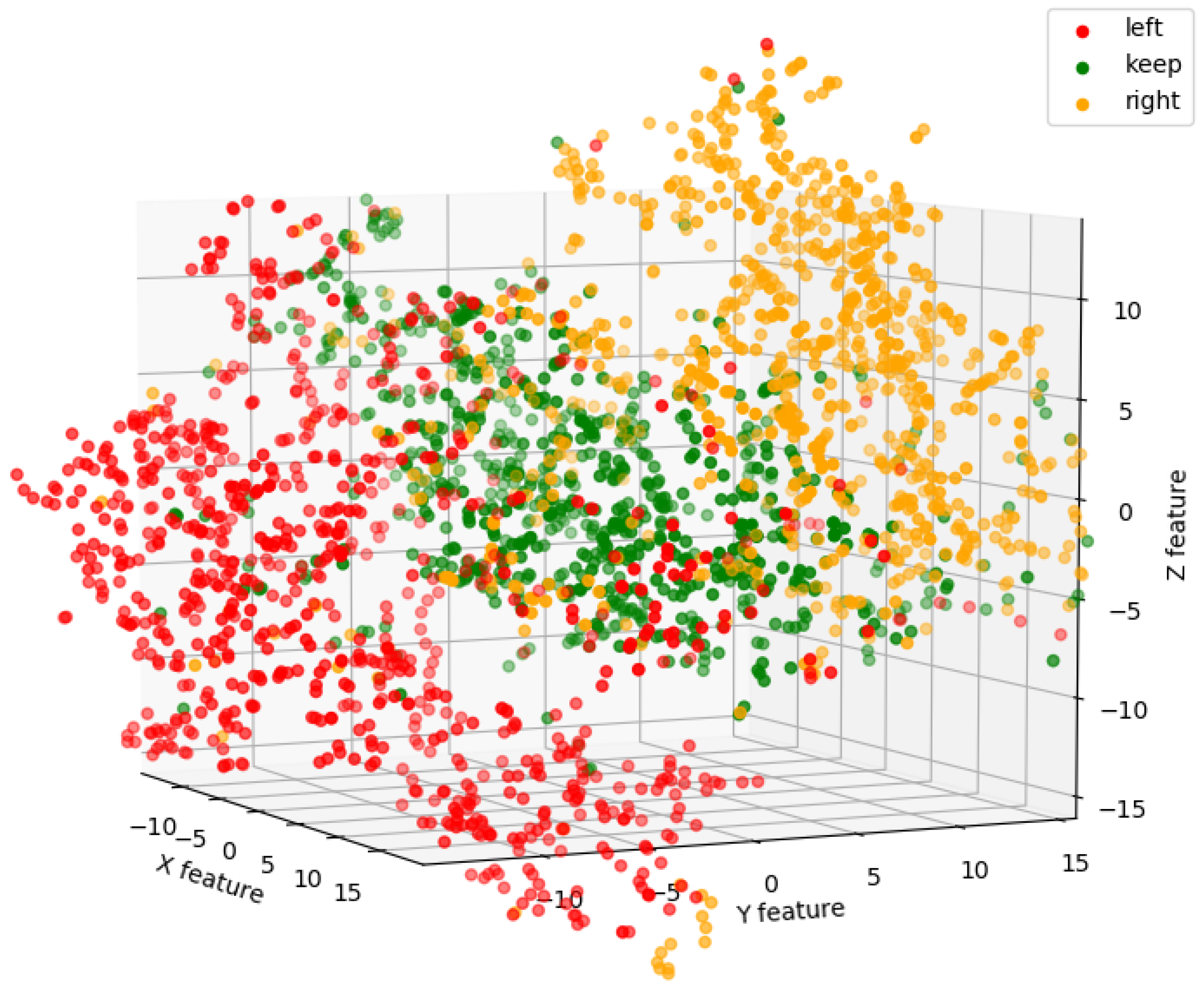
• Second, coming from the continuous encoding nature of the VAE, the encoding of similar trajectories are also close to each other in the context vector, hence it can provide maneuver classification information without training information.

In Section 2, the problem is outlined regarding sequential data encoding and interpretation and gives the motivation of this research. Briefly, the purpose of this article is to provide examples of efficient trajectory data compression for behavior prediction using autoencoder neural networks. Trajectory prediction is not the subject of this article as it attempts to analyze trajectories in more depth. Sequential data compression and classification are separate tasks. All the experiments are performed using the Next Generation Simulation (NGSIM) trajectory database [25,26]. The database is presented in Section 3, along with each preprocessing step. In Section 4, the models used in the research are introduced, with special emphasis on the VAE, divided into three sub-sections. The LSTM and Convolutional Sparse Autoencoders (Section 4.1 and Section 4.2) and the Convolutional Variational Autoencoders (CVAE) Section 4.3 are shown in separate sub-sections. The explanation of the CVAE’s loss function is a key point, and therefore its introduction is justified in more detail. Section 5 presents the results of model training and data research. All details regarding the training can be found in Section 5.1, while the coding ability in Section 5.2 is illustrated with figures. The result of the network’s coding capability is used for a classification problem and discussed in Section 5.3, and finally Section 5.4 is devoted to the analysis of latent spatial behavior.

2. Problem Formulation

Convolutional neural networks (CNN) and LSTM Recurrent Neural Networks [27,28] for the optimization are studied in this paper. Different tools can be applied for the maneuver classification problem, such as Support Vector Machine, Gaussian Classifier, and LSTM neural networks [10,11,12,13,14]. For more precise trajectory forecasting and analysis, one way is to use some method of dimension reduction.

The obvious choice for sequence analysis is an RNN architecture. Still, in the case of longer sequences, the vanishing and exploding gradient problem become the main obstacle of the optimization, according to [29]. To avoid this, one can use, e.g., LSTM RNN, but its complexity (the number of parameters) can be high. Therefore, the training, as well as the inference process, can be slow. It is not an important aspect during the research work if GPUs are available for accelerating the optimization and the inference. Lately, several forecasting and classification concepts have been thoroughly proven in the literature. However, carefully choosing the neural networks’ architecture to minimize the model complexity can be useful in the practice.

A CNN can also find and learn temporal features and patterns in a one-dimensional “image”; in our case, this dimension is the time [16]. Every pixel is one-time step, and the number of channels is equal to the d feature number. CNN based autoencoder can yield the same or better result as a Bidirectional LSTM with a tenth of its complexity.

The context vector can be used for maneuver detection, classification, and data visualization. This paper presents autoencoders trained to copy the trajectories while the context vector is low dimensional and carries useful information. Using the same architecture for predicting future trajectory fails because of the lack of information about the surrounding vehicles [15,30,31]. A hypothesis is set up predicting the future trajectory’s context vector instead of the future trajectory itself. From this, it is decoded that the performance should be better. It is shown that the experimental result overturns this hypothesis, so the trajectories do not decode enough latent information about surrounding vehicle motions.

3. The Training Dataset

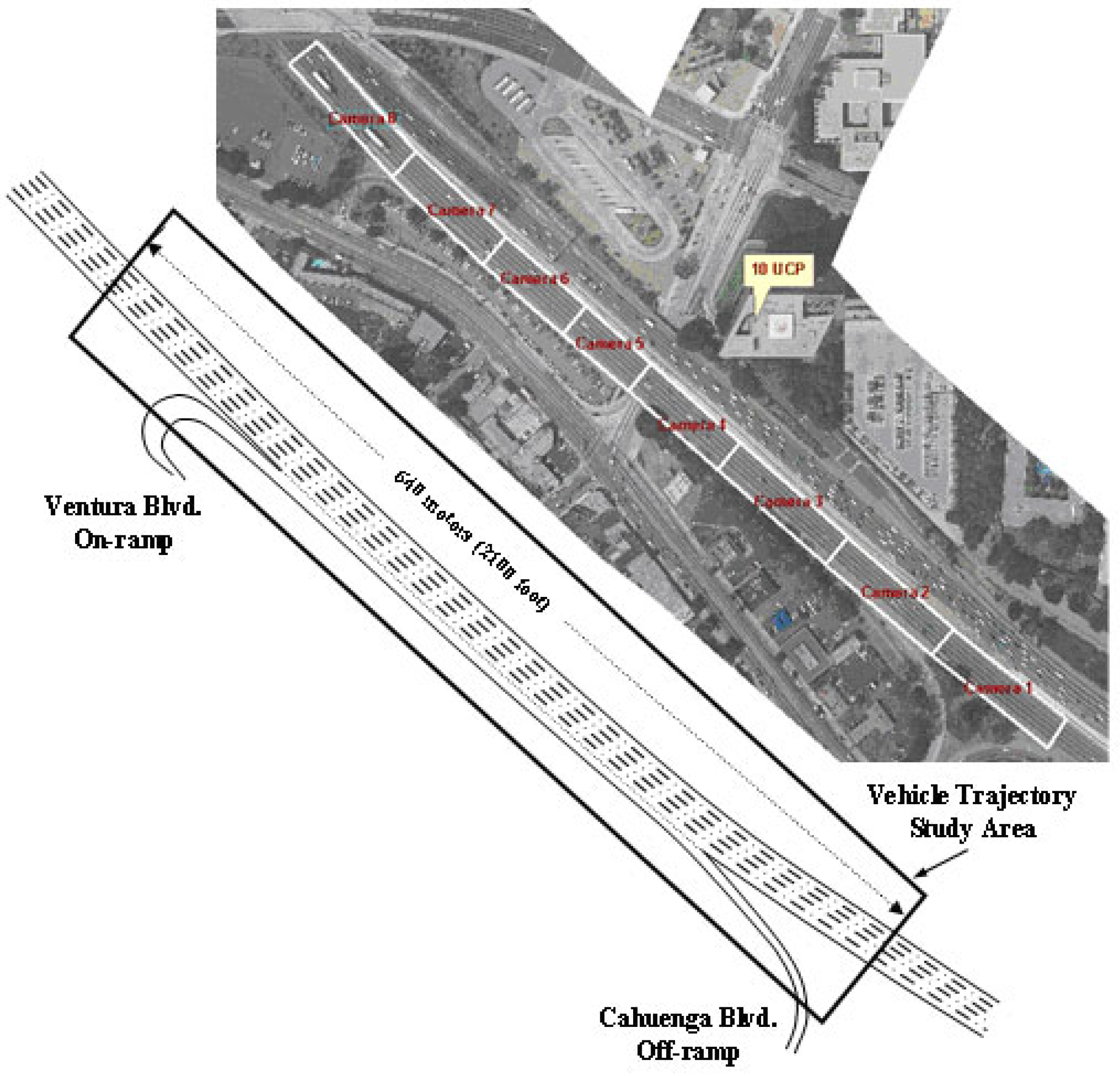
The data set for training is $\mathcal{X}\equiv {\mathbb{R}}^{d\times s}$ and every $x\in \mathcal{X}$ data point is a vehicle trajectory with sequence length s and feature dimension d. Sequence length is $s=60$, which means 6 s, and the feature dimension is $d=2$, which is the longitudinal and lateral coordinate of the vehicle in every time step. The traffic situation is a multi-lane highway road in the US, and the data collection was made by the New Generation Simulations (NGSIM).

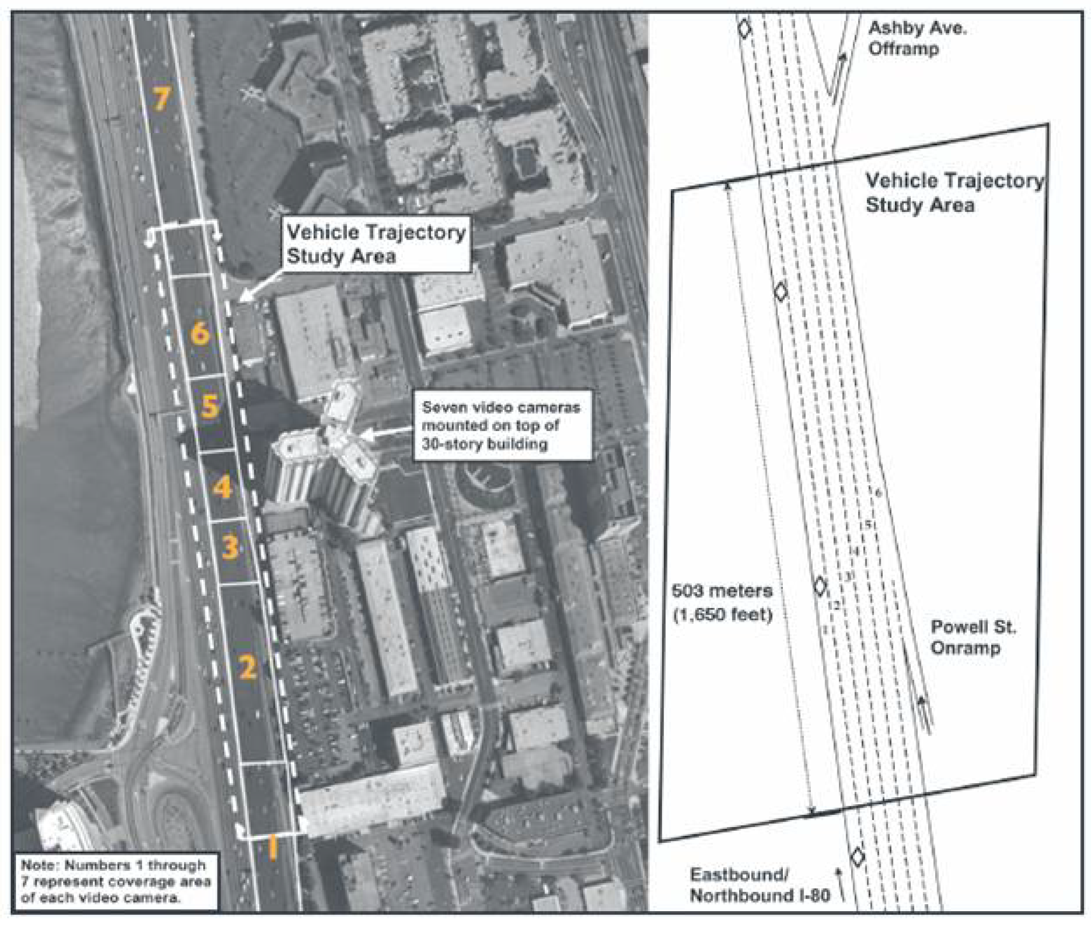
The NGSIM Unites States Highway 101 (US-101) (Figure 1) and Interstate 80 (I-80) (Figure 2) datasets [25,26] are used for training and evaluating the trajectory autoencoding problem. This trajectory data has precise location, velocity, and acceleration of each vehicle within a specific area every $0.1$ s. Furthermore, it provides relative positions to surrounding vehicles and lane position in every frame. There are $11.8$ million rows and 25 columns in this dataset. Each row represents one vehicle in a specific frame with all the information. The columns in ascending order are the following: vehicle identification number, frame identification number ascending by start time, the total number of frames in which the vehicle appears, global time, lateral (x) and longitudinal (y) coordinate of the vehicle’s front center concerning the left-most edge of the section in the direction of travel, global $x,y$ coordinate, length and width of the vehicle, vehicle type (1—motorcycle, 2—auto, 3—truck), instantaneous velocity and acceleration, and lane position.

Data Preprocessing and Preparations

The database for the training consists of 1614 vehicles. One-third of them perform a lane-changing maneuver to the left, and another one third is right lane changing; the rest is lane-keeping. Two trajectory pieces are extracted from the complete path data of each vehicle. One is 6 s (60 time-steps) ahead of the occurrence of the lane index changing, and one other 6 s after. In the case of the lane-keeping ones, two consecutive pieces of trajectory are taken. All the $x,y$ coordinate units have been changed from feet to meters. The following steps have been performed on both subsets.

First, we checked if a vehicle had at least 120 time-steps in the data set because two 60 long sequences are desired, and separated according to what maneuver is done. Second, a vehicle is only considered in the training set if the lane changing occurred later than the first 60 time-steps, with the two sequences extracted. Thirdly, the two sets have been added together and the largest possible balanced data set is randomly chosen and drawn, with the same number of lane-keeping, left, and right lane changing vehicles.

For the sake of the higher generalization capability, every trajectory sample is translated to start from the origin.

4. Methodology

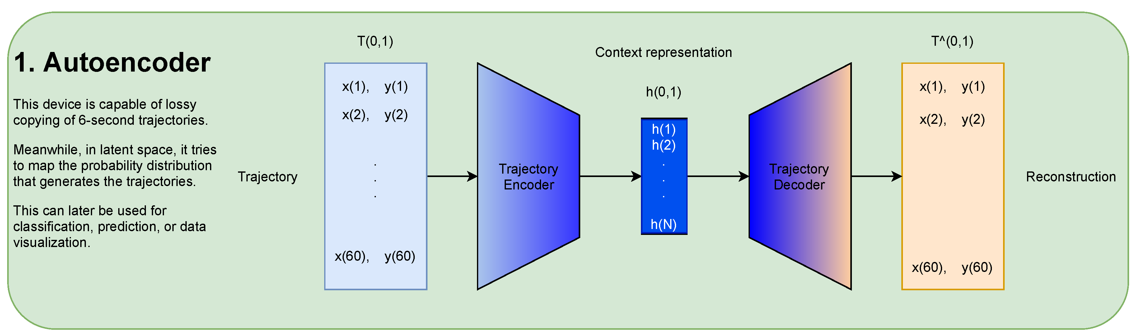
The idea behind the presented research uses autoencoders to train a neural network to a simple task copying the input data into the output as accurately as possible [20]. An Autoencoder (AE) contains an encoder neural network and a decoder network. The encoder takes the input vector and transforms it into another vector (usually with a smaller dimension) called the context vector. The decoder receives this code and dilates it back to the size of the input data. This scheme fits into any AE’s basic concept, and it is summarized in Figure 3. At each epoch, one feeds the data forward, the encoder, and the decoder takes the reconstruction error, backpropagates it through the network, and updates its weights. The process can be trained by any gradient descent optimization method. All the models are optimized by Adam [32] with different learning rates between 0.0001–0.001, depending on the convergence performance.

The training uses mean square error (MSE) loss, which is the reconstruction loss. An additional loss function is also taken to smooth the output. The derivative of the target and decoded sequence is formed, their MSE is calculated and added to the reconstruction loss after multiplication by the weight of $0.1$:

$$L_0=MSE(x,f\left(z\right))+w_{1}MSE(\mathrm{D}x,\mathrm{D}f\left(z\right)),$$

(1)

where ${\left(\mathrm{D}x\right)}_i=x_i-x_{i+1}$

4.1. Bidirectional LSTM Autoencoder

Based on LSTM networks’ success in learning sequential data generation process’s nonlinear, time-dependent dynamics [27,28], the application of LSTM networks is evident. The structure of the model is described below. The Encoder is a Bidirectional LSTM RNN with an adjustable c context dimension—meaning that the LSTM [33] cell has a hidden state and cell state dimension equal to c. Coordinates $x,y$ are fed in every time-step. The hidden and cell states are initialized randomly in the first time step, and the resulting new one is passed to the next step. The last ones are taken as the context vector and used as the initialization of the Encoder LSTM. During training mode, teacher forcing [34] is applied with a ratio of $0.5$. The decoder in the first step takes the original trajectory’s last time step $x,y$ coordinates. The other steps take the previous output or the corresponding ground truth from the original trajectory. In the case of validation and test, teacher forcing is turned off. The context dimension is set to be $c=10,12,15,20$ using three LSTM layers and 0.5 dropout.

4.2. Convolutional Sparse Autoencoder

The encoder and decoder are one-dimensional CNNs with four compound convolutional layers and one linear layer. The numbers of input channels of the layers are 2, 6, 12, and 8 and the kernel sizes 4, 6, 8, and 5, respectively. PReLU activation function is applied in every layer with one parameter per channel. The last two layers use maximum pooling to reduce sequence length. Their kernel size is 3, and 2 with the dilation of 1. Thus, the output shape of the compound convolutional layers is $5\times 5=25$. A single fully connected layer is used to reduce this number to the c context dimension.

The decoder’s transposed convolutional layers upscale the channel number and the sequence length. The channel numbers are 1, 3, 8, 4, and 2:

$$Loss(x,z)=\frac{1}{N}\sum _{i=1}^N\left(\frac{\left|\right|x_i-f\left(z_i\right){\left|\right|}^2}{2c}\right)+\lambda \frac{1}{C}\sum _{i=1}^C\left|z_i\right|$$

(2)

4.3. Convolutional Variational Autoencoder

Variational Autoencoder inherently has an explicit regularization during the training process [35]. VAEs encode the input as a distribution over the latent space instead of encoding it as a point. The context vector is then sampled from this distribution, the sampled context is decoded, and the reconstruction error is computed. One data point from the data set is denoted by x and the encoded representation, called “context vector” is z. Let’s denote the prior distribution over the latent space by $p\left(z\right).$

Probabilistic decoder: This is defined by $p\left(x\right|z)$, and it describes the distribution of the decoded variable given the encoded variable.

Probabilistic encoder: This is defined by $p\left(z\right|x)$, and it describes the distribution of the encoded variable given the decoded variable.

The probabilistic encoder and decoder concept is not enough to solve the regularization problem regarding the content generation. It is easy to see that the model is not prevented from returning distributions like Dirac delta or punctual functions behave like classic models leading to overfitting. In the next paragraphs, the details of the mathematical concepts of the VAE are covered, and the deduction of the correct loss function for the optimization is presented.

Below, two assumptions are made about the distributions:

$$\begin{array}{cc}\hfill p\left(z\right)& \equiv \mathcal{N}(0,\mathbb{I})\hfill \end{array}$$

(3)

$$\begin{array}{cc}\hfill p\left(x\right|z)& \equiv \mathcal{N}\left(f\right(z),c\mathbb{I})f\in F;c>0.\hfill \end{array}$$

(4)

F denotes a set of functions that can be parametrized by a finite number of parameters, so it does not cover all the functions in general. The F elements can be approximated by neural networks, which is the key to finding the optimal decoding. On the other hand, the Bayesian theorem can unfold the probabilistic encoder

$$p\left(z\right|x)=\frac{p\left(x\right|z\left)p\right(z)}{p\left(x\right)}=\frac{p\left(x\right|z\left)p\right(z)}{\int p\left(x\right|u\left)p\right(u)du}$$

(5)

which is used in Equation (7) for the deduction of a practical formula. Otherwise, the integral in Equation (5) cannot be evaluated, so it cannot be used in practice. By means of the variational inference formulation, the $p\left(z\right|x)$ encoder distribution is approximated by an other Gaussian $q_x\left(z\right)$, where the mean and the variance are functions of variable x:

$$q_x\left(z\right)\equiv \mathcal{N}(g\left(x\right),h\left(x\right))g\in G;h\in H.$$

(6)

Here, G and H are sets of parametrized functions just like F. Among these functions, one needs to find the best approximation of the $g,h$ functions by determining their parameters. The best approximation is supposed to minimize the Kullback–Leibler divergence [36] between the approximation and the original $p\left(z\right|x)$ distribution. The optimal $g^{*}$ and $h^{*}$ functions obtained by

$$(g^{*},h^{*})=\underset{(g,h)\in G\times H}{arg\; min}KL(q_x\left(z\right),p\left(z\right|x)).$$

(7)

Here, Equation (5) is substituted and one gets

$$(g^{*},h^{*})=\underset{(g,h)\in G\times H}{arg\; min}\left(\mathbb{E}(log(q_x(z)))-\mathbb{E}\left(log\frac{p\left(x\right|z\left)p\right(z)}{p\left(x\right)}\right)\right),$$

(8)

$$(g^{*},h^{*})=\underset{(g,h)\in G\times H}{arg\; min}\left(\mathbb{E}(log\left(q_x\left(z\right)\right)-\mathbb{E}(logp\left(z\right))-\mathbb{E}(logp\left(x\right|z))+\mathbb{E}(logp\left(x\right))\right).$$

(9)

After rearranging the terms, the Kullback–Leibler divergence of $q_x\left(z\right)$ and $p\left(z\right)$ distributions appears, which can be calculated. The last term does not depend on g and h, so, generally, it gives only a constant contribution so that it can be omitted in the minimization problem:

$$(g^{*},h^{*})=\underset{(g,h)\in G\times H}{arg\; min}\left(-\mathbb{E}(logp\left(x\right|z)+KL(q_x\left(z\right),p\left(z\right))\right)$$

(10)

$$(g^{*},h^{*})=\underset{(g,h)\in G\times H}{arg\; min}\left(\mathbb{E}\left(\frac{\left|\right|x-{f\left(z\right)\left|\right|}^2}{2c}\right)+KL(q_x\left(z\right),p\left(z\right))\right).$$

(11)

The last equation expresses that the optimizer needs to find a balance between the reconstruction loss, which is the maximization of the log-likelihood for the $p\left(x\right|z)$ and the KL divergence of $q_x\left(z\right)$ and the prior which enforce the encoder to stay close to the standard normal distribution. This is a trade-off between how much one can rely on the data and how fair assumption is the prior.

In case of the function f, one should maximize the expected log-likelihood of output x given a z context vector sampled from $g_x\left(z\right)$:

$$f^{*}=\underset{f\in F}{arg\; max}\mathbb{E}(logp\left(x\right|z))=\underset{f\in F}{arg\; max}\mathbb{E}\left(-\frac{\left|\right|x-{f\left(z\right)\left|\right|}^2}{2c}\right).$$

(12)

Taking Equation (11) into account, the final optimization problem is formulated in maximizing the following expression with respect to the parameters of the three functions $(f,g,h)$:

$$(f^{*},g^{*}{h}^{*})=\underset{(f,g,h)\in F\times G\times H}{arg\; max}\left(\mathbb{E}\left(-\frac{\left|\right|x-{f\left(z\right)\left|\right|}^2}{2c}\right)-KL(q_x\left(z\right),p\left(z\right))\right).$$

(13)

The mean square error approximates the first term. The second term is the Kullback–Leibler divergence between the normal distribution $q_x\left(z\right)$ with a diagonal covariance matrix and the standard normal distribution. After performing the calculation, one gets the loss function for the VAE;

$$Loss(x,z)=\sum _i\left(\frac{\left|\right|x_i-f\left(z_i\right){\left|\right|}^2}{2c}\right)+\frac{1}{2}\sum _i\left(h\left(x_i\right)-g{\left(x_i\right)}^2-log\left(h\left(x_i\right)\right)-1\right)$$

(14)

In addition, using the mean squared error of the first derivatives gives a better and smoother result, thus the final loss function for the VAE with Equation (1) takes the following form:

$$Los{s}_{CVAE}(x,z)=L_0(x,f\left(z\right),\mathrm{D}x,\mathrm{D}f\left(z\right))+\lambda \frac{1}{2}\sum _i\left(h\left(x_i\right)-g{\left(x_i\right)}^2-log\left(h\left(x_i\right)\right)-1\right)$$

(15)

All the functions $f,g,h$ are parametrized by the parameters of neural networks, and $F,G,H$ sets are defined by their architectural design. Empirically determined parameters for the encoder and decoder are given in

Table 1. Parameters of the Variational Autoencoder Architecture.

The Parameters of the Common Part of the Encoder
	Channels
	Input	Output	Kernel	Dilation
Conv1D	2	6	4	-
PReLU	6	6		-
Conv1D	6	12	6	-
PReLU	12	12	-	-
Conv1D	12	8	8	-
PReLU	8	8	-	-
MaxPool1D	-	-	3	1
The Two Separate Part for the $\mathbf{\mu }$ and $\mathbf{\sigma }$ Generation
Conv1D	8	5	5	-
PReLU	5	5	-	-
MaxPool1D	-	-	2	1
Dense	25	$D_{i}nt$	-	-
PReLU	$D_{i}nt$	$D_{1}nt$	-	-
Dense	$D_{i}nt$	C	-	-

and

Table 2. The parameters of the decoder.

	Input	Output	Padd.	Kernel	Stride	Dilat.
Dense	C	10
ConvTranspose1D	1	3	2	3	1	1
PReLU	3	3
AdaptiveAvgPool1D	Dimension: 10
ConvTranspose1D	3	8	2	5	2	1
PReLU	8	8
AdaptiveAvgPool1D	Dimension: 15
ConvTranspose1D	8	4	2	5	2	1
PReLU	4	4
AdaptiveAvgPool1D	Dimension: 30
ConvTranspose1D	4	2	0	5	1	1
AdaptiveAvgPool1D	Dimension: 60

.

5. Results

5.1. Training

All the models and the training are implemented using the Pytorch [37] framework. In training mode, random Gaussian noise with zero mean and 0.1 variance is added to every trajectory sample in the training set. Meanwhile, during the validation and test mode, the noise is not applied. This method helps the neural network to learn denoising capabilities and reconstruct the trajectories more smoothly. In this subsection, the training loss values are presented in

Table 3. Loss values of Variational Autoencoder Training.

V-AE	Latent Dimension
C	3	4	5	6	7	8	9	10
Valid	12.87	8.78	6.91	6.27	6.64	6.02	5.67	6.11
Training	14.51	10.67	7.95	6.55	6.42	6.34	5.91	5.87
Complexity	2825	2861	2959	2997	3101	3141	3251	3293

and

Table 4. Loss values of Bidirectional LSTM AE Training.

BiLSTM-AE	Latent Dimension
C	10	12	15	20
Valid	31.2	21.74	14.81	9.6
Training	76.8	32.45	21.94	12.36
Complexity	12522	17714	27182	47442

. The tables contain the lowest value of the validation losses and the corresponding training losses. All values are derived from the reconstruction loss and the regularization term. An average per sample is taken on the data set, so this value is the expected value of the reconstruction and regularization error of a sample trajectory with $2\times 60$-parameters. Furthermore, the learning curves of SAE, LSTM AE, and CVAE are presented in Figure 4 in the case of 10-dimensional latent space. A moving average smoothes the curves with a window size of 1000 epochs for the sake of better visibility.

The Convolutional Sparse Autoencoder (SAE) described in Section 4.2 fails to converge during the training process. Using the regularization term in loss function Equation (2) gives a better result than without using it though the training loss freezes around 50–100 based on the learning rate and latent space dimension. In Figure 4, the red lines show that the SAE gets stuck in a local optimum during the optimization, unable to make that progress like the CVAE (cyan blue curves) does. Since the loss values are the sum of the losses along the 2 times 60 components of the meters’ trajectory, the value above 35 means that the average deviation is around 0.5 m for each component. This is too big to say that SAE training is satisfactory. A similar finding can be made for the LSTM AE.

The LSTM AE (Section 4.1) with the same regularization gives slightly better results regarding the loss values in Table 4. The LSTM can only approach CVAE’s loss values with much greater complexity. Once the latent space dimension is chosen below 10, the training process can not converge, so the losses become unmanageable big values and extremely fluctuating. On Figure 4, the purple lines correspond to the LSTM AE. Much less epoch number is used for the training due to the larger run-time. The training error could be further reduced, but the validation loss’s rise indicates the overfitting phenomenon; therefore, it does not make sense. These results suggest that the sparse regularization term in Equation (2) assumes a prior distribution in the latent space that does not approximate the real one well.

The lowest loss values (Table 3) are resulted by the Convolutional Variational Autoencoder (Section 4.3) with the inherent regularization term in Equation (14). This is included in the assumption of the standard normal distribution for the prior distribution in the latent space. The result of the CVAE is reported below.

5.2. Encoding and Decoding Performance

In Figure 5, the CVAE encoding performance is illustrated on three maneuvers. From top to bottom: Reconstruction with 10-, 6-, and 4-dimensional latent space. From left to right: The same trajectory of a lane-keeping and lane changing on the right and left. The red curve is the ground truth trajectory, while the green one is the most probable reconstruction given the latent distribution. With blue lines, several reconstructions are plotted using 100 different context vectors sampled from the latent distribution. The transparency of the line is proportional to its likelihood. The horizontal axis is the longitudinal y coordinate of the vehicle’s trajectory, and the vertical is the lateral x coordinate. Under the trajectory graphs, the hidden state vector is plotted.

It can be seen that, by reducing the dimension, the reconstruction ability deteriorates, which can also be observed in the values in Table 3. However, this does not have such a significant effect on the classification, see

Table 5. Results of SVM classification on latent representations.

C-SVM	Latent Dimension
C	3	4	5	6	7	8	9	10
0.1	0.767	0.811	0.755	0.860	0.854	0.829	0.888	0.857
1	0.820	0.829	0.866	0.876	0.888	0.869	0.913	0.882
20	0.817	0.827	0.901	0.891	0.888	0.888	0.910	0.894

.

5.3. Maneuver Classification

In a maneuver classification task, a learning algorithm is trained to specify which maneuver from a fixed class belongs to the input trajectories. Supervised learning algorithms solve this task by producing a function mapping from the input space $\mathcal{X}$ to a finite category class $\mathcal{C}$, which is a subset of the natural numbers $\mathbb{N}$. In this case, the input trajectory is a tensor of $\mathcal{X}\equiv {\mathbb{R}}^{2\times 60}$ and the category set is $\mathcal{C}=\{\mathrm{left}\mathrm{lane}\mathrm{changing},\mathrm{lane}\mathrm{keeping},\mathrm{right}\mathrm{lane}\mathrm{changing}\}$ and can be identified by a numeric label code $\{0,1,2\}$ respectively. Although the CVAE is not trained as a classifier, it can cluster the data by learning its intrinsic properties, which is useful for classification as well.

The CVAE has learned latent information about the maneuvers in an unsupervised way, illustrated by the 3D latent space visualization in Figure 6. An arbitrary 6-second trajectory is mapped into the latent space as a Gaussian distribution by the trained CVAE encoder part. The centrum of this distribution is the expected value vector. These vectors can be visualized using a projection from the latent space to the three-dimensional space. On the three-dimensional space in Figure 6, every dot colored by the maneuver label belongs to a trajectory. According to the maneuvers, the points representing different trajectories are automatically separated in the latent space, although the labels belonging to the maneuvers haven’t been used during the training. This is due to the construction of the CVAE with adequate regularizing ability, in which the prior distribution of the latent space variable is assumed to be standard normal, and the probabilistic encoder and decoder follow a normal distribution. The CVAE preprocessed the trajectories by selecting the characteristic features, making it easier to find planes that separate the classes with a small error. A Support Vector Machine [38] on context vectors can classify trajectories according to maneuvers with 88–91% accuracy (see Table 5), which is more than the tools can that have been specifically trained for maneuver detection [14].

5.4. Latent Space Visualization

In Figure 7, an interpolation is visualized in the latent representation space. The series begins with a right lane change and ends with a left lane change. The three internal states result from decoding the weighted average of the two extreme states’ context vectors. Continuous transition is observed in terms of the distance traveled longitudinally and laterally and in the trajectory shape. The continuous transition between two completely different trajectories suggests that the regularization properly organizes the latent space. The decoded trajectories from the internal states are not uncertain as expected without regularization but eligible ones, thus the decoder can be used for content generation. The VAE described in Section 4.3 learns meaningful mapping and coding.

The t-distributed Stochastic Neighbor Embedding (t-SNE) is a widespread technique for the latent space visualization [39]. After 120 data trajectories are encoded by the VAE into a 3 to 10-dimensional vector space, this procedure is applied to visualize the data in three dimensions.

6. Conclusions

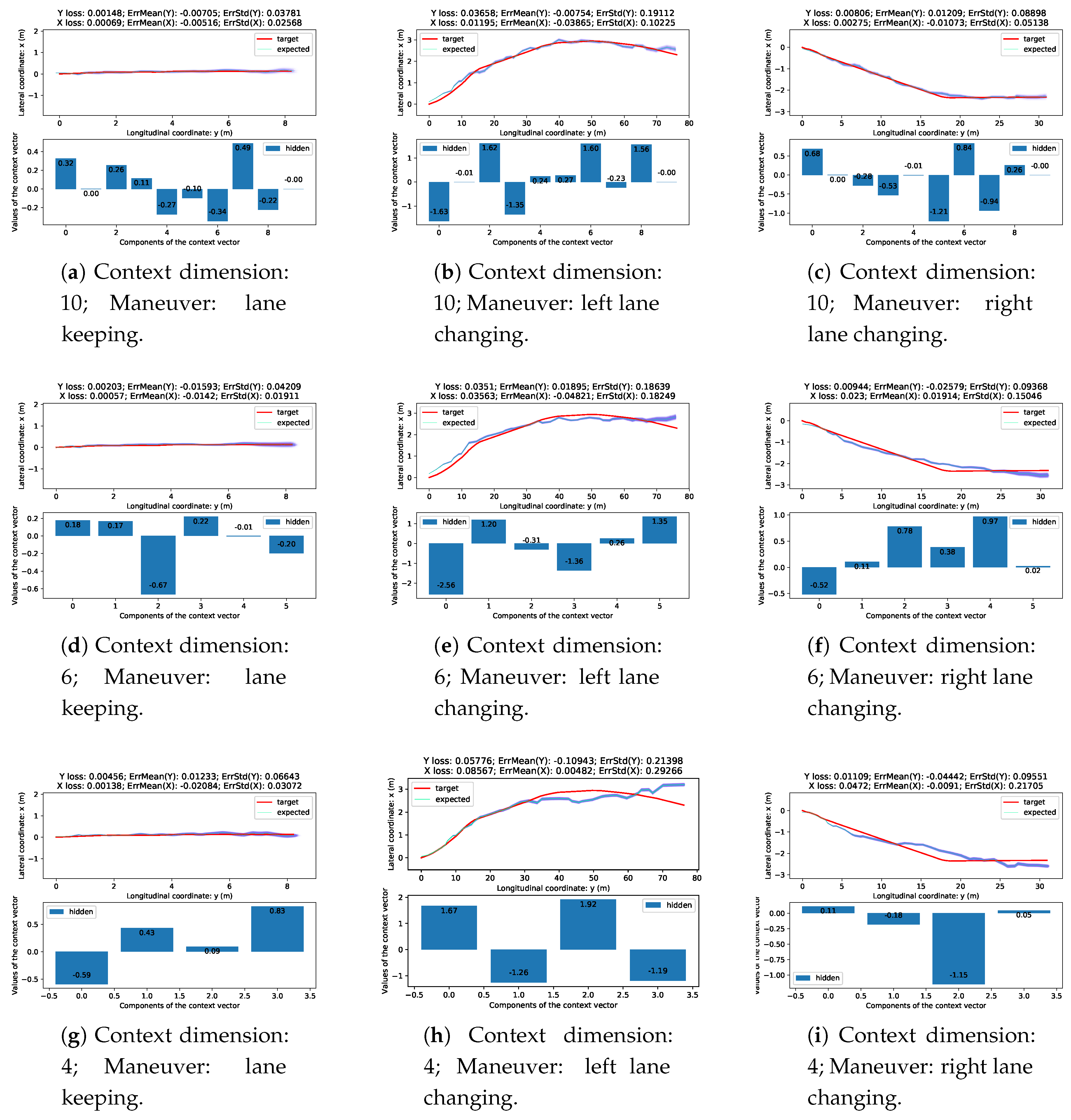
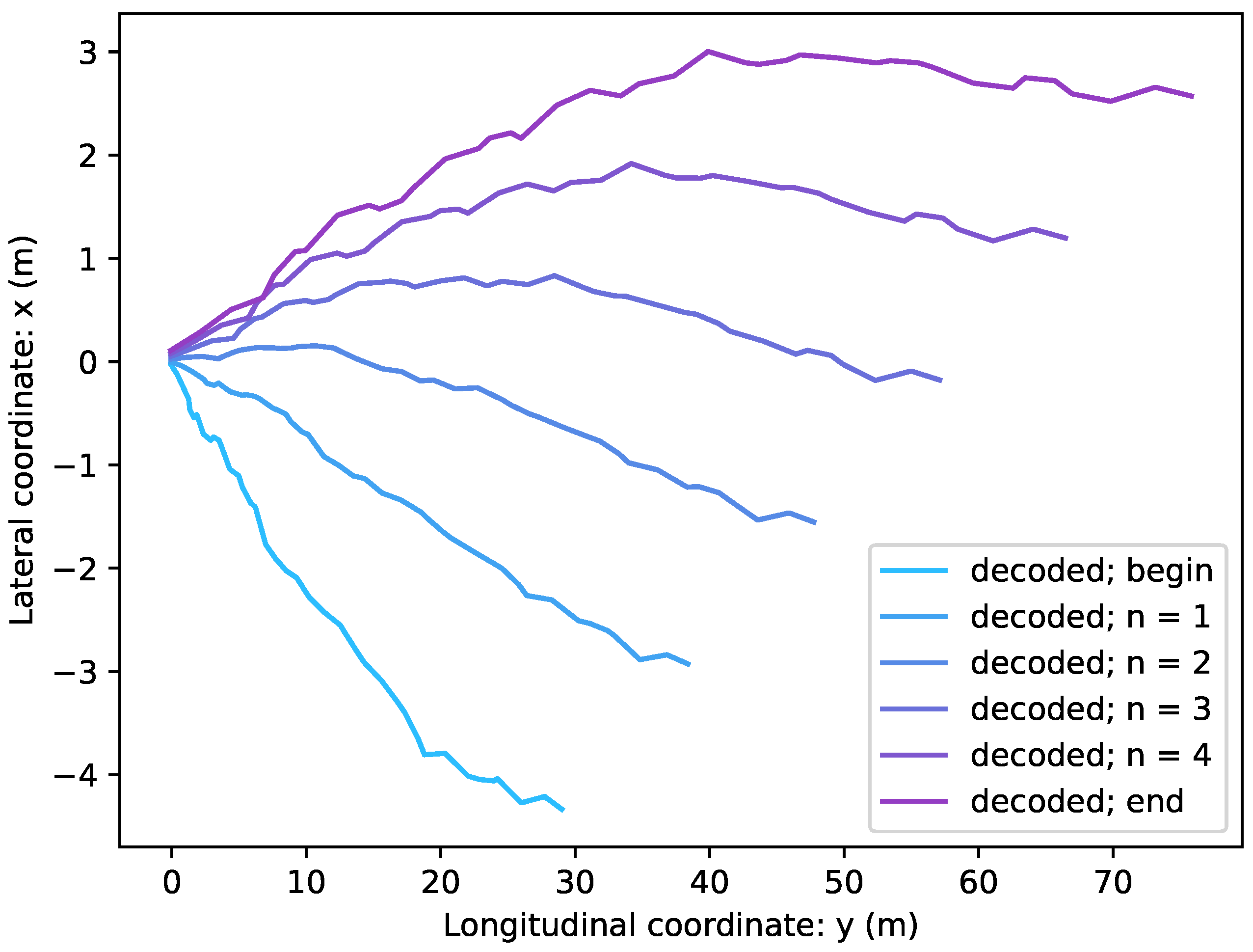
The research presented in this paper shows that a CVAE, with an appropriate neural network structure, is capable of the lossy compression of real-world vehicle trajectories. The compressed code, also known as the context vector, or latent representation, can also be used for maneuver detection and classification. In addition, a representation that continuously maps similar patterns is learned, successfully modeling the vehicle trajectories automatically and meaningfully.

In the future, the input for trajectory data analysis and behavior prediction should be further investigated. A more realistic model should have the three lateral classes for lane changing behavior, multiplied by several longitudinal ones. Longitudinal classes could separate acceleration behaviors. Environmental conditions can also affect driver behavior, as light and dense traffic have different inner structures. Hence, a more sophisticated model should handle maneuvers that are specific to this situation.

The paper also shows that the encoded context vector can be used for maneuver classification. It could be used for trajectory prediction, but it is essential to consider more information about the traffic situation to make predictions. One should take the trajectory of surrounding vehicles into account in some manner. It would be possible to test whether such networks can encode the vehicle’s trajectory under investigation with the information of vehicles moving around it. An autoencoder network should be trained for yielding the future trajectory of the vehicle to the output by feeding the historical trajectory of the ego vehicle and the surroundings to the input. It is possible to separate the input encoding (and copying) task to the prediction task. In other words, on the one hand, one can train to predict the future trajectory, but one can also train the method to predict in latent space. In the latter case, it is quite simply a matter of a separately trained device encoding the trajectories and mapping them into the latent space, followed by another performing the prediction on the context vector from which the decoder decrypts the future trajectory.

References

1. Geng, X.; Liang, H.; Yu, B.; Zhao, P.; He, L.; Huang, R. A scenario-adaptive driving behavior prediction approach to urban autonomous driving. Appl. Sci. 2017, 7, 426. [Google Scholar] [CrossRef]
2. Hegedűs, T.; Németh, B.; Gáspár, P. Challenges and Possibilities of Overtaking Strategies for Autonomous Vehicles. Period. Polytech. Transp. Eng. 2020, 48, 320–326. [Google Scholar] [CrossRef]
3. Buehler, M.; Iagnemma, K.; Singh, S. The DARPA Urban Challenge: Autonomous Vehicles in City Traffic; Springer-Verlag, Berlin, Germany 2009, Volume 56. Springer-Verlag: Berlin, Germany, 2009; Volume 56. [Google Scholar]
4. Ploeg, J.; de Haan, R. Cooperative Automated Driving: From Platooning to Maneuvering. In Proceedings of the 5th International Conference on Vehicle Technology and Intelligent Transport Systems—Volume 1: VEHITS, INSTICC, Heraklion, Greece, 3–5 May 2019; SciTePress: Setubal, Portugal, 2019; pp. 5–10. [Google Scholar] [CrossRef]
5. Llamazares, A.; Molinos, E.J.; Ocaña, M. Detection and Tracking of Moving Obstacles (DATMO): A Review. Robotica 2020, 38, 761–774. [Google Scholar] [CrossRef]
6. Dagli, I.; Brost, M.; Breuel, G. Action recognition and prediction for driver assistance systems using dynamic belief networks. In Net. ObjectDays: International Conference on Object-Oriented and Internet-Based Technologies, Concepts, and Applications for a Networked World; Springer: Berlin, Germany, 2002; pp. 179–194. [Google Scholar]
7. Trautman, P.; Krause, A. Unfreezing the robot: Navigation in dense, interacting crowds. In Proceedings of the 2010 IEEE/RSJ International Conference on Intelligent Robots and Systems, Taipei, Taiwan, 18–22 October 2010; pp. 797–803. [Google Scholar]
8. Wiest, J.; Höffken, M.; Kreßel, U.; Dietmayer, K. Probabilistic trajectory prediction with Gaussian mixture models. In Proceedings of the 2012 IEEE Intelligent Vehicles Symposium, Alcala de Henares, Spain, 3–7 June 2012; pp. 141–146. [Google Scholar] [CrossRef]
9. Cruz, L.A.; Zeitouni, K.; de Macedo, J.A. Trajectory Prediction from External Sensor Data using Recurrent Neural Networks. In Proceedings of the International Conference on Big Data & Cybersecurity Intelligence, Hadath, Lebanon, 13–15 December 2018; pp. 18–20. [Google Scholar]
10. Deo, N.; Trivedi, M.M. Multi-Modal Trajectory Prediction of Surrounding Vehicles with Maneuver based LSTMs. In Proceedings of the 2018 IEEE Intelligent Vehicles Symposium (IV), Changshu, China, 26 June–1 July 2018; pp. 1179–1184. [Google Scholar]
11. Rodrigues, M.; McGordon, A.; Gest, G.; Marco, J. Adaptive tactical behaviour planner for autonomous ground vehicle. In Proceedings of the 2016 UKACC 11th International Conference on Control (CONTROL), Belfast, UK, 31 August–2 September 2016; pp. 1–8. [Google Scholar] [CrossRef] [Green Version]
12. Dou, Y.; Yan, F.; Feng, D. Lane changing prediction at highway lane drops using support vector machine and artificial neural network classifiers. In Proceedings of the 2016 IEEE International Conference on Advanced Intelligent Mechatronics (AIM), Banff, AB, Canada, 12–15 July 2016; pp. 901–906. [Google Scholar] [CrossRef]
13. Izquierdo, R.; Parra, I.; Muñoz-Bulnes, J.; Fernández-Llorca, D.; Sotelo, M.A. Vehicle trajectory and lane change prediction using ANN and SVM classifiers. In Proceedings of the 2017 IEEE 20th International Conference on Intelligent Transportation Systems (ITSC), Yokohama, Japan, 16–19 October 2017; pp. 1–6. [Google Scholar]
14. Rákos, O.; Aradi, S.; Bécsi, T. Lane Change Prediction Using Gaussian Classification, Support Vector Classification and Neural Network Classifiers. Period. Polytech. Transp. Eng. 2020, 48, 327–333. [Google Scholar] [CrossRef]
15. Deo, N.; Rangesh, A.; Trivedi, M.M. How Would Surround Vehicles Move? A Unified Framework for Maneuver Classification and Motion Prediction. IEEE Trans. Intell. Veh. 2018, 3, 129–140. [Google Scholar] [CrossRef] [Green Version]
16. Cui, H.; Radosavljevic, V.; Chou, F.; Lin, T.; Nguyen, T.; Huang, T.; Schneider, J.; Djuric, N. Multimodal Trajectory Predictions for Autonomous Driving using Deep Convolutional Networks. In Proceedings of the 2019 International Conference on Robotics and Automation (ICRA), Montreal, QC, Canada, 20–24 May 2019; pp. 2090–2096. [Google Scholar]
17. Buzachis, A.; Filocamo, B.; Fazio, M.; Ruiz, J.A.; Sotelo, M.A.; Villari, M. Distributed Priority Based Management of Road Intersections Using Blockchain. In Proceedings of the 2019 IEEE Symposium on Computers and Communications (ISCC), Barcelona, Spain, 29 June–3 July 2019; pp. 1159–1164. [Google Scholar]
18. Parra, I.; Corrales, H.; Hernández, N.; Vigre, S.; Llorca, D.F.; Sotelo, M.A. Performance analysis of Vehicle-to-Vehicle communications for critical tasks in autonomous driving. In Proceedings of the 2019 IEEE Intelligent Transportation Systems Conference (ITSC), Auckland, New Zealand, 27–30 October 2019; pp. 195–200. [Google Scholar]
19. Pu, Y.; Gan, Z.; Henao, R.; Yuan, X.; Li, C.; Stevens, A.; Carin, L. Variational autoencoder for deep learning of images, labels and captions. In Advances in Neural Information Processing Systems; Curran Associates Inc.: Red Hook, NY, USA, 2016; pp. 2352–2360. [Google Scholar]
20. Baldi, P. Autoencoders, Unsupervised Learning and Deep Architectures. In Proceedings of the 2011 International Conference on Unsupervised and Transfer Learning Workshop (UTLW’11), Bellevue, WA, USA, 2 July 2011; Volume 27, pp. 37–50. [Google Scholar]
21. Li, X.; Chen, Z.; Poon, L.K.; Zhang, N.L. Learning latent superstructures in variational autoencoders for deep multidimensional clustering. arXiv 2018, arXiv:1803.05206. [Google Scholar]
22. Jiang, Z.; Zheng, Y.; Tan, H.; Tang, B.; Zhou, H. Variational Deep Embedding: An Unsupervised and Generative Approach to Clustering. arXiv 2016, arXiv:1611.05148. [Google Scholar]
23. Xu, W.; Sun, H.; Deng, C.; Tan, Y. Variational autoencoder for semi-supervised text classification. In Proceedings of the Thirty-First, AAAI Conference on Artificial Intelligence, San Francisco, CA, USA, 4–9 February 2017. [Google Scholar]
24. Krajewski, R.; Moers, T.; Nerger, D.; Eckstein, L. Data-Driven Maneuver Modeling using Generative Adversarial Networks and Variational Autoencoders for Safety Validation of Highly Automated Vehicles. In Proceedings of the 2018 21st International Conference on Intelligent Transportation Systems (ITSC), Maui, HI, USA, 4–7 November 2018; pp. 2383–2390. [Google Scholar]
25. Colyar, J.; Halkias, J. Us Highway 80 Dataset; Federal Highway Administration (FHWA): Washington, DC, USA, 2006.
26. Colyar, J.; Halkias, J. US Highway 101 Dataset; Tech. Rep. FHWA-HRT-07-030; Federal Highway Administration (FHWA): Washington, DC, USA, 2007. [Google Scholar]
27. Cho, K.; Van Merriënboer, B.; Gulcehre, C.; Bahdanau, D.; Bougares, F.; Schwenk, H.; Bengio, Y. Learning phrase representations using RNN encoder–decoder for statistical machine translation. arXiv 2014, arXiv:1406.1078. [Google Scholar]
28. Graves, A. Generating sequences with recurrent neural networks. arXiv 2013, arXiv:1308.0850. [Google Scholar]
29. Pascanu, R.; Mikolov, T.; Bengio, Y. On the difficulty of training recurrent neural networks. In Proceedings of the International Conference on Machine Learning, Atlanta Georgia, 16–21 June 2013; pp. 1310–1318. [Google Scholar]
30. Gupta, A.; Johnson, J.; Fei-Fei, L.; Savarese, S.; Alahi, A. Social GAN: Socially Acceptable Trajectories with Generative Adversarial Networks. In Proceedings of the IEEE Conference on Computer Vision and Pattern Recognition (CVPR), Salt Lake City, UT, USA, 18–22 June 2018. [Google Scholar]
31. Lee, N.; Choi, W.; Vernaza, P.; Choy, C.B.; Torr, P.H.S.; Chandraker, M. DESIRE: Distant Future Prediction in Dynamic Scenes With Interacting Agents. In Proceedings of the IEEE Conference on Computer Vision and Pattern Recognition (CVPR), Honolulu, HI, USA, 21–26 July 2017. [Google Scholar]
32. Kingma, D.P.; Ba, J. Adam: A method for stochastic optimization. arXiv 2014, arXiv:1412.6980. [Google Scholar]
33. Hochreiter, S.; Schmidhuber, J. Long short-term memory. Neural Comput. 1997, 9, 1735–1780. [Google Scholar] [CrossRef] [PubMed]
34. Williams, R.J.; Zipser, D. A learning algorithm for continually running fully recurrent neural networks. Neural Comput. 1989, 1, 270–280. [Google Scholar]
35. Doersch, C. Tutorial on variational autoencoders. arXiv 2016, arXiv:1606.05908. [Google Scholar]
36. Kullback, S.; Leibler, R.A. On information and sufficiency. Ann. Math. Stat. 1951, 22, 79–86. [Google Scholar] [CrossRef]
37. Paszke, A.; Gross, S.; Massa, F.; Lerer, A.; Bradbury, J.; Chanan, G.; Killeen, T.; Lin, Z.; Gimelshein, N.; Antiga, L.; et al. PyTorch: An Imperative Style, High-Performance Deep Learning Library. In Advances in Neural Information Processing Systems 32; Curran Associates, Inc.: Red Hook, NY, USA, 2019; pp. 8024–8035. [Google Scholar]
38. Cortes, C.; Vapnik, V. Support-vector networks. Mach. Learn. 1995, 20, 273–297. [Google Scholar] [CrossRef]
39. van der Maaten, L.; Hinton, G. Visualizing Data using t-SNE. J. Mach. Learn. Res. 2008, 9, 2579–2605. [Google Scholar]
Figure 1. Top view of the US-101 freeway from which the data are extracted.
Applsci 10 06739 g001
Figure 2. Top view of the I-80 freeway from which the data are extracted.
Applsci 10 06739 g002
Figure 3. Concept of the autoencoding scheme to learn latent features from the distribution of trajectories. The encoder and decoder are enforced to copy the data with the reconstruction loss as low as possible with an informational bottleneck.
Applsci 10 06739 g003
Figure 4. Training and validating losses are shown for the autoencoders being compared. All three equipped 10-dimensional latent space for comparability. The number of epochs is on the horizontal axis and the loss values are on logarhythmically scaled vertical axis.
Applsci 10 06739 g004
Figure 5. Variational Autoencoder performance on copying the trajectory data without using the traffic information of surrounding vehicles. From top to bottom: Reconstruction with 10-, 6-, and 4-dimensional latent space. From left to right: The same trajectory of a lane-keeping and lane changing on the right and the left, respectively. The red curve is the ground truth; the green one is the most probable reconstruction trajectory. The horizontal axis is the longitudinal y coordinate of the vehicle’s trajectory, and the vertical is the lateral x coordinate. Under the trajectory graphs: The hidden state vector is plotted.
Applsci 10 06739 g005
Figure 6. The 10-dimensional latent space visualized by t-SNE embedding in three dimensions. Every dot represents a trajectory, and the colors encode the maneuver classes.
Applsci 10 06739 g006
Figure 7. An interpolation between two different maneuvers is visualized. The series of trajectory plots begin with a right lane change and ends with a left lane change. There are three internal states that are the result of decoding the weighted average of the context vectors of the two extreme states. The continuous transition illustrates the well-organized nature of the latent space generated by the encoder.
Applsci 10 06739 g007