The Spec-Radiation Method as a Fast Alternative to the Re-Radiation Method for the Detection of Flaws in Wooden Particleboards

Abstract

For real-time evaluation of non-destructive air-coupled ultrasonic testing of wood-based materials, efficient and reliable calculation methods from ultrasonic holography are essential. Presented here is the spec-radiation method as a fast alternative to the re-radiation method. The spec-radiation method offers a more accurate and up to 88% faster evaluation than the re-radiation method for the determination of flaws in particleboards. Flaws of sub-wavelength sizes can be identified and their shape and location can be determined with this method. The spec-radiation method produces a better reproduction of the sound field than the re-radiation method, especially in the area of the measuring plane.

1. Introduction

Panel-shaped, wood-based materials are becoming increasingly important in today’s world. Whether it is in the furniture industry, where furniture with processed wood is becoming more common as an approach to sustainability, or in the construction industry, where wood is considered a cost-effective, durable material unlike expensive high-performance materials such as Carbon Fiber Reinforced Polymer (CFRP) or Glass Fiber Reinforced Polymers (GFRP). Most big name furniture manufacturers want to offer their products at lower prices and this is usually only possible through material savings, without compromising the load-withstanding capacity of the material. This means that a 100% control of the processed wooden particleboards is necessary. This must be non-destructive, fast, and reliable.

This is what non-destructive ultrasonic testing is used for today, which has been continuously developed since Sokolov [1] first used it for material testing. In contact ultrasonic testing, both transmitter and receiver are in contact with the test material. The difference in impedance between the transmitter/receiver and the test material often requires a layer of contact oil. However, this can leave residues on the test material and even be absorbed by the wood material and change its properties (Schafer [2]). The contact force also has a great influence on the accuracy of the results (Gyekenyesi et al. [3]). These led to the development of non-contact testing methods, with air serving as the ambient or contact medium (Fang et al. [4]). Usually, water is used as contact or ambient medium, due to its suitable impedance properties to many materials (Zhang et al. [5], Jasiuniene et al. [6], Mitri et al. [7]). However, due to the large difference in impedance with air as the contact medium, most of the ultrasonic energy is reflected at the interface between the media (Sanabria et al. [8]). To counteract this problem, development of powerful ultrasonic transducers (Hillger et al. [9]) and suitable matching layers between the ultrasonic transducer and the air (Chimenti [10], Álvarez Arenas [11]) were developed, allowing meaningful investigations to be carried out quickly, accurately, and reproducibly. During the industrial production of wooden particleboards, air inclusions and imperfectly glued areas can now occur (Dunky and Niemz [12]).

The first to use ultrasound to detect delaminations and air inclusions in wood were Niemz [13], Bucur and Böhnke [14]. They drew conclusions about flaws or delaminations by means of changes in the propagation time of the signal. In the industrial production of particleboards, due to pressing and gluing, these boards have temperatures of up to $100 °$C, with vapors escaping that lead to receiver damage (Dunky and Niemz [12]). This led to the use of air-coupled ultrasound as a testing method, with large distances to the particleboard (>100 mm). According to Döring [15], the three most common methods to obtain information from non-destructive testing (NDT) with ultrasound are A-, B-, and C-scans. The subdivision describes the amount of information used for evaluation. While an A-scan processes and displays the information of one measuring point, a B-scan already processes the information of a line of connected measuring points. In a C-scan, an area of measuring points is processed and displayed. The C-scan is particularly suitable for determining flaws or delaminations in shape and position. However, when viewed at a large distance from the particleboard, considerable errors occur. This is due to the diffraction of the sound waves behind the flaw (Laybed and Huang [16]). If the receiver measures a plane and the transmitter is stationary during the experiment, tomographic measurements can be done and be displayed in a C-scan (Chimenti [10]). In order to identify the flaws in a particleboard, methods of acoustic holography can be used.

Due to the coherent property of ultrasonic radiation, the back propagation calculation of sound waves is possible, eliminating the diffraction-induced inaccuracies (Singh [17]). A successful method to identify flaws is the re-radiation method (Sanabria et al. [18], Marhenke et al. [19,20,21], Schmelt et al. [22,23]). This is suitable for flaws down to the sub-wavelength range (Marhenke et al. [19], Schmelt et al. [22]) and can be carried out quickly in the experiment by using interpolation methods (Schmelt et al. [22]). Besides the identification of flaws, it is also possible to identify objects in a sound field (Tsysar and Sapozhnikov [24], Schmelt et al. [25]). This method is based on the Rayleigh–Sommerfeld diffraction integral which has made its way from optics to acoustics. It offers a well interpretable mathematical expression by the representation in the spatial domain.

Another method used in the field of optics to propagate the light waves is the angular spectrum method (Delen and Hooker [26]). This was used first by Booker and P. C. Clemmow [27] and then considered by Ratcliffe [28] for application in the diffraction of light rays in the ionosphere. Boyer et al. [29] showed that it is possible to apply this method in the field of acoustics to compute the propagation of sound waves similar to light waves. Identification of holes in the plate was carried out using a 5 MHz transmitter in a through transmission measurement and a steel plate with holes as a sound mirror. Since then, this method has been used in various areas of acoustics. Schafer and Lewin [30] and de Belleval and Messaoud-Nacer [31] employed the method to characterize transmitters. A program called “FOCUS” has been developed to simulate transmitters (McGough et al. [32], Zeng and McGough [33], Alles et al. [34]). It is used for the analysis of tissue harmonic imaging (Yan and Hamilton [35]), as well as the identification of objects (Peng et al. [36]). As a finite element model, it has already been used by Aanes et al. [37]. Liu and Waag [38] have described the forward and backward propagation of sound waves with this method.

Fast and reliable algorithms are indispensable for the idea of a real-time analysis of particleboards in production. With the established re-radiation method, this has been partially achieved. However, the hardware is not economically viable for the required number of computing operations. In this publication, we present the spec-radiation, which takes a further step towards real-time analysis by using the angular spectrum method for the detection of flaws in particleboards. We show that the spec-radiation method offers good detection possibilities even with a coarse measurement grid, in contrast to the re-radiation method, where this is only achievable with additional effort.

We also show that this method can be applied with the extension for increasing the detectability of a coarse measuring grid as presented in Schmelt et al. [22], as it is used in the re-radiation method. We show that the spec-radiation method delivers good reproductions of the sound field, including the area of the measuring plane. We show this through two experiments with flaw imitations in two dimensions. One has a larger diameter than the wavelength $\lambda$ and the other has a smaller one. Large distances (approximately 500 mm) between the transmitter through the particleboard to the receiver have to be bridged with the sound attenuation in air depending on the frequency (Jakevičius and Demcčenko [39], Stößel [40]). For this, we use a low excitation frequency of 50 kHz. The presented spec-radiation method is up to 88% faster then the re-radiation method. We compare the re-radiation method with the spec-radiation method on the basis of measured data from a transmission test of a wooden particleboard with and without flaws. We show the influence of the measuring grid point distance on both methods. Using an academic piston transducer as an example, we investigate the calculation speed of both methods.

This publication is structured as follows: In Section 2 the materials and methods are introduced, with the spec-radiation method in Section 2.1, the re-radiation method in Section 2.2, the experimental setup in Section 2.3, and the practical implementation of the spec-radiation method in Section 2.4. In Section 3 the results are reported. In Section 3.1 the experimental data with a measured grid point distance of 2 mm is studied and the influence of the evaluation window size is investigated. In Section 3.2 the effects of coarse measuring grids are explored. In Section 3.3 are the results from the use of a coarse measuring grid to enhance detectability using the method from Schmelt et al. [22], and in Section 3.4, the difference in the computing speed is investigated. In Section 4 is the discussion.

2. Materials and Methods

In this section the methods of this publication are presented as well as the experimental conditions. In Section 2.1, the spec-radiation method based on the angular spectrum method is presented. Section 2.2 presents the re-radiation method based on the Rayleigh–Sommerfeld diffraction integral. In Section 2.3, the experimental setup is described. Finally, Section 2.4 presents the practical implementation of the spec-radiation method. The differences to the re-radiation method are elaborated.

2.1. The Spec-Radiation Method

The spec-radiation method is based on the angular spectrum method. The following derivation is mainly based on Goodman [41], who described it for light, and on Liu and Waag [38], who described it for acoustics.

The Helmholtz equation describes the propagation of acoustic pressure waves in an incompressible fluid:

$${\nabla }^{2}p(x,y,z,t)-{\displaystyle \frac{1}{c^2}}{\displaystyle \frac{{\partial }^2}{\partial t}}p(x,y,z,t)=0,$$

(1)

where $x,y,z$ are the space coordinates, t is the time, c is the speed of sound in the corresponding medium, which is assumed to be constant here, and $p(x,y,z,t)$ describes the acoustic pressure field in space and time. If Equation (1) is transferred to the Fourier domain, the following results are obtained:

$${\nabla }^{2}p(\mathbf{x},\omega )+kp(\mathbf{x},\omega )=0,$$

(2)

with the space coordinate vector $\mathbf{x}=[x,y,z]$ and:

$$k={\displaystyle \frac{2\pi }{\lambda }}={\displaystyle \frac{\omega }{c}}$$

(3)

where $\omega$ is the time dependent angular frequency. The acoustic sound pressure $p(\mathbf{k},\omega )$ can be written as follows:

$$p(\mathbf{k},\omega )={\int \int \int \int }_{-\infty }^{\infty }p(\mathbf{x},t){\mathrm{e}}^{-\mathrm{i}(\mathbf{k}·\mathbf{x}+\omega t)}\mathrm{d}x\mathrm{d}y\mathrm{d}z\mathrm{d}t.$$

(4)

Here, the wave vector $\mathbf{k}=[k_x,k_y,k_z]$ and $k_x,k_y,k_z$ are the spatial angular frequencies and i is the complex unit. Equation (4) satisfies Equation (2) when the exponent factor also satisfies Equation (2), and we get:

$$k_z=2\pi \sqrt{{\left({\displaystyle \frac{1}{\lambda }}\right)}^2-f_x^2-f_y^2},$$

(5)

with $k_x=2\pi f_x$ and $k_y=2\pi f_y$. The sound pressure distribution in the plane z:

$$p(k_x,k_y,z,\omega )={\mathrm{e}}^{-\mathrm{i}{k}_{z}z}{\int \int }_{-\infty }^{\infty }p(x,y,z,\omega ){\mathrm{e}}^{-\mathrm{i}(k_{x}x+k_{y}y)}\mathrm{d}x\mathrm{d}y.$$

(6)

This now describes the propagation in the z-direction with the spatial frequencies $f_x$ and $f_y$. Two cases must be distinguished:

$$\begin{array}{cc}\hfill 1.& f_x^2+f_y^2\le {\displaystyle \frac{1}{{\lambda }^2}}\hfill \\ \hfill 2.& f_x^2+f_y^2>{\displaystyle \frac{1}{{\lambda }^2}}\hfill \end{array}$$

(7)

The first case describes homogeneous waves and the second case describes exponentially decaying evanescent waves. If the spectrum of a plane, e.g., the measuring plane with the coordinates $x=x^{\prime }$, $y=y^{\prime }$ and $z=z^{\prime }$, is known at $z^{\prime }=0$:

$$\mathfrak{F}\left(p(x^{\prime },y^{\prime },0,\omega )\right)={\int \int }_{-\infty }^{\infty }p(x^{\prime },y^{\prime },0,\omega ){\mathrm{e}}^{-\mathrm{i}(k_x{x}^{\prime }+k_y{y}^{\prime })}\mathrm{d}x\mathrm{d}y$$

(8)

with $\mathfrak{F}$ as the Fourier transform operator and Equation (8) substituted into Equation (5), resulting in:

$$p(k_x,k_y,z,\omega )=\mathfrak{F}\left(p(x^{\prime },y^{\prime },0,\omega )\right){\mathrm{e}}^{-\mathrm{i}{k}_{z}z}.$$

(9)

To display the result in the spatial domain and not in the Fourier domain, an ${\mathfrak{F}}^{-1}$ is necessary:

$$p(x,y,z,\omega )={\mathfrak{F}}^{-1}\left(\mathfrak{F}\left(p(x^{\prime },y^{\prime },0,\omega )\right){\mathrm{e}}^{-\mathrm{i}{k}_{z}z}\right).$$

(10)

Depicted here is that only factor ${\mathrm{e}}^{-\mathrm{i}{k}_{z}z}$ is responsible for the propagation of the sound wave. Equation (10) becomes with propagation function $H(k_x,k_y,z)$:

$$p(x,y,z,\omega )={\mathfrak{F}}^{-1}\left(\mathfrak{F}\left(p(x^{\prime },y^{\prime },0,\omega )\right)H(k_x,k_y,z)\right).$$

(11)

The propagation function can now take two forms, depending on whether the sound waves are to be calculated forward in time or backward. For both forward or backward propagation, the propagation function is now defined as:

$$H(k_x,k_y,z)={\mathrm{e}}^{-\mathrm{i}{k}_{z}z}.$$

(12)

2.2. The Re-Radiation Method

The re-radiation method, which is based on the Rayleigh–Sommerfeld diffraction integral, is derived in this work according to Sanabria et al. [18], Marhenke et al. [19,20,21], Schmelt et al. [22,23], Tsysar and Sapozhnikov [24], Schmelt et al. [25], Schmerr and Song [42], Sommerfeld [43]. Here, the derivation is equal to the derivation of the spec-radiation method from Equation (1) to Equation (6). As Delen and Hooker [26] described, the inverse Fourier transform of Equation (13) is:

$${\mathfrak{F}}^{-1}\left({\mathrm{e}}^{-\mathrm{i}{k}_{z}z}\right)={\displaystyle \frac{1}{2\pi }}{\displaystyle \frac{\partial }{\partial z}}\left[{\displaystyle \frac{{\mathrm{e}}^{-\mathrm{i}kR}}{R}}\right]$$

(13)

and thus describes the derivative of free-space Green’s function, with $R=\sqrt{{(x-x^{\prime })}^2+{(y-y^{\prime })}^2+z^2}$ as the distance description. A spatial representation is thus derived here. Sommerfeld [44] found that the right term in Equation (13) describes oscillating dipoles. Transferred to acoustics, this corresponds to oscillating point sources. This makes it easier to understand the parameters in the equation. If Equation (13) is inserted into Equation (10), the result is:

$$p(\mathbf{x},\omega )={\mathfrak{F}}^{-1}\left(\mathfrak{F}\left(p({\mathbf{x}}^{\prime },\omega )\right)\mathfrak{F}\left({\displaystyle \frac{1}{2\pi }}{\displaystyle \frac{\partial }{\partial z}}\left[{\displaystyle \frac{{\mathrm{e}}^{V\mathrm{i}kR}}{R}}\right]\right)\right),$$

(14)

with ${\mathbf{x}}^{\prime }=[x^{\prime },y^{\prime },(z^{\prime }=0)]$. Here, V describes the propagation parameter, which for $z\le 0$ is $V=-1$ and for $z>0$ is $V=1$. This simplified interpretation of the re-radiation method through representation in the spatial domain is, however, at the expense of additional computational operations, including an additional 2D Fourier Transformation (FFT) that must be performed. A faster calculation is also possible using the spec-radiation method.

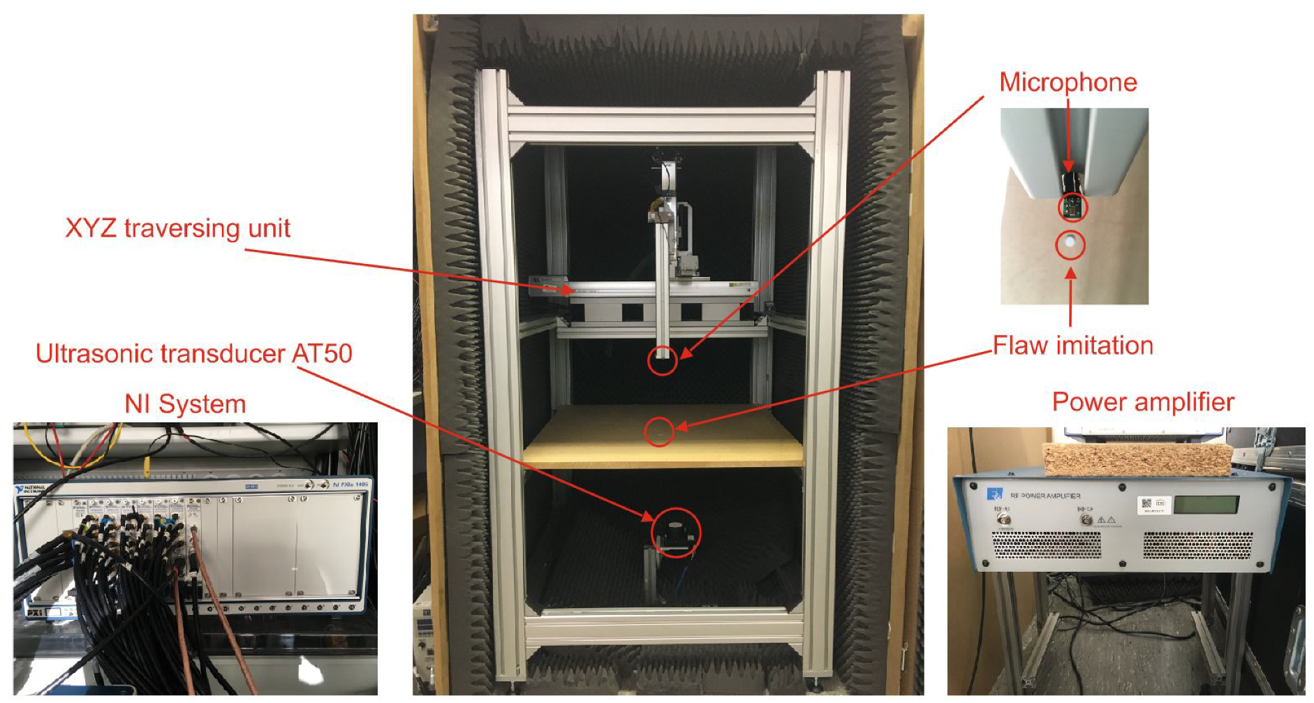
2.3. Experimental Setup

In the experiment, air was used as the coupling medium between the transmitter and the particleboard and the receiver. As a transmitter, an Airmar pulse ultrasonic transducer was used. The used model AT50 has an active diameter of 45 mm and operates at 50 kHz. Therefore, the wavelength in air at 50 kHz is approx. $\lambda =6.9$ mm. With an amplitude of 80 V, the transmitter was sending 10 sinusoidal oscillations with a repeating frequency of 1 Hz. The distance between the transmitter and the particleboard was always 280 mm and, therefore, greater than the near field length, which is, according to Krautkrämer and Krautkrämer [45], approximately 72 mm, of the transmitter in air at this frequency. During the whole measurement, the transmitter was stationary. The particleboard was a commercially available wooden medium-density fiberboard (MDF). The dimensions of the particleboard measured at height = 800 mm, width = 800 mm, and depth = 20 mm. For wooden particleboards, the choice for suitable flaw imitations are pieces of paper (Marhenke et al. [19,21], Schmelt et al. [22,23]) instead of Teflon tape which is historically used for CFRP and GFRP (Fahr [46]). This is through the assumption that paper has nearly the same material properties as the particleboard. Here, the thin air film between the piece of paper and the particleboard serves as flaw imitation. The air film causes a similar impedance change in the material properties like a real air inclusion at the top of the particleboard. The pieces of paper used as flaw imitations were circular with a diameter of ø20 mm, which is larger than the wavelength, and ø4 mm, which is smaller than the wavelength. The wooden particleboard was also immovable. A Knowles microphone, SPU0410LR5H-QB, was used as a receiver, due to its recording frequency up to 80 kHz and its small dimension with the height = 1.1 mm, width = 3 mm, length = 3.76 mm, and an acoustic port of ø0.25 mm. Since both transmitter and particleboard were immobile, the receiver must move to obtain the information for a C-scan. It was attached to an XYZ traversing stage from RoboCylinder with the maximum traversing path of x = 0–400 mm, y = 0–200 mm, and z = 0–200 mm. During the whole measurement, the XYZ traversing stage did not move in the z direction. The entire system was controlled by a standard computer. Via USB, the XYZ stage unit was connected to the computer and controlled by a LabView program. With a National Instruments (NI) system, the transmitter was controlled and the signal of the microphone recorded. The NI system consisted of a chassis PXIe-1085, with an inserted card for the communication with the computer (PXIe-8398), a card to record the measurement data (PXIe-5171R with a maximum sampling frequency of 250 MHz and 8 channels), and a card (PXIe-5423) as a frequency generator to control the transmitter. For the amplification of the control signal of the transmitter, the power amplifier 1040L of the company E&I was used to generate the required amplitude of 80 V. Figure 1 depicts the experimental setup. The experimental setup is identical to that in Schmelt et al. [22], for completeness it is explained here. The only difference is that in the present study, only the experiments with a flaw imitation ø$20\mathrm{mm}>\lambda$ and a flaw imitation ø$4\mathrm{mm}<\lambda$ and a measurement from a flawless particleboard are performed.

2.4. Practical Implementation

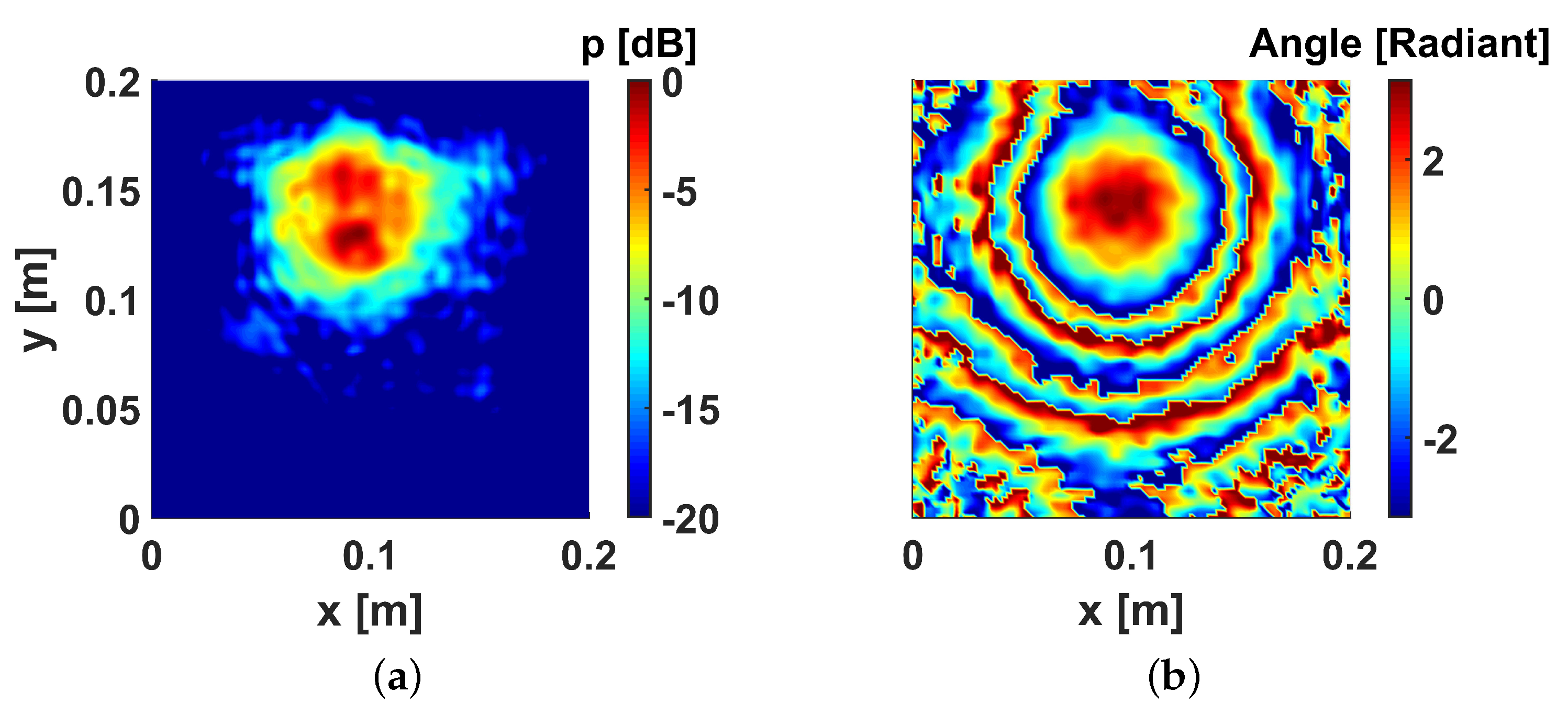
Figure 2 and Figure 3 show the program flow and clarifies the practical realization of the spec-radiation method and the difference to the re-radiation method. The extension for the enhancement of the detectability of a coarse measuring grid made by Schmelt et al. [22] is already included in the flow chart.

The program starts in Figure 2 by loading the measured transient sound pressure field $p(x^{\prime },y^{\prime },0,\omega )$ in the measuring plane at $z^{\prime }=0$ into the working memory. Afterwards, important parameters are set, such as the sound velocity of air, which can be calculated according to Cramer [47]. In these carried out experiments, the speed of sound was approximately 343 m/s. In the next section, a decision has to be made whether an enhancement of the detectability is desired on the basis of whether a coarse measuring grid is to be used or not. If an enhancement of the detectability is desired, the data is interpolated by a spline interpolation to a finer virtual grid and so $p(x^{\prime },y^{\prime },0,t)$ is interpolated to $p(x_{Virt}^{\prime },y_{Virt}^{\prime },0,)$. Afterwards, the transient sound pressure field is brought into the time frequency domain by a one-dimensional FFT, whereby the complex amplitudes in the spatial domain are obtained. These amplitudes then go into the block “Radiation Technique”, depicted in Figure 3. Here, the re-raditaion and the spec-radiation techniques use different codes. For the re-radiation technique, a grid with the spatial coordinates is created first. With this grid, the term can then be calculated from Equation (13). Next, the 2D FFT of this term is calculated to determine the propagation function $H(k_x,k_y,z)$. A 2D FFT of the complex amplitudes in the spatial domain is performed as well to transfer the complex amplitudes into the Fourier domain. Then, the multiplication of $H(k_x,k_y,z)$ and $p(k_x,k_y,0,\omega )$ is performed, which corresponds to the convolution, and the complex amplitudes in the Fourier domain at the distance z are obtained. The complex amplitudes are transferred from the Fourier domain back into the spatial domain utilizing a 2D inverse Fourier Transform (iFFT). For the calculation with the spec-radiation method, a grid of the spatial angular frequencies $k_x$ and $k_y$ is created first. Then, a two-dimensional FFT of the complex amplitudes in the spatial domain is performed to obtain the complex amplitudes in the Fourier domain. In contrast to the re-radiation method, the propagation function $H(k_x,k_y,z)$ can be calculated directly through the grid of the spatial frequencies according to Equations (5) and (12), making a 2D FFT not necessary. The wavenumber step is defined with the size of the measurement field to $\Delta k_x=\frac{2\pi }{x_{max}}$ and $\Delta k_y=\frac{2\pi }{y_{max}}$. By multiplying the complex amplitudes in the Fourier domain with the propagation function, i.e., the convolution, the complex amplitudes in the Fourier domain at the distance z are obtained. The complex amplitudes are transferred from the Fourier domain back into the spatial domain utilizing a 2D iFFT. The results can now be displayed as the amplitude or phase in the spatial domain to identify flaws. To compute the time data, the results must be brought back into the time domain with a corresponding iFFT. It is easy to see that the spec-radiation method is faster in the numerical calculation than the re-radiation method because only one 2D FFT is necessary. The advantages of the spec-radiation method will be discussed in the following section.

3. Results

In this section, the results are reported. In Section 3.1, experimental data with a measured grid point distance of 2 mm is studied. The influence of the evaluation window size on the re-radiation method as well as on the spec-radiation method is investigated. In Section 3.2, the effect of coarse measuring grids are explored. Section 3.3 discusses the results from the use of a coarse measuring grid to enhance detectability using the method from Schmelt et al. [22]. In Section 3.4, the computing speed is determined using an example of an idealized piston transmitter.

3.1. Results with 2 mm Grid Point Distance

In this section, the grid point distance is 2 mm in the x and y direction. First, the experimental result without a flaw imitation is evaluated. The size of the evaluation window corresponds to the measurement window and has 101 × 101 grid points. A single frequency (50 kHz) is evaluated here to draw a straightforward comparison. In Figure 4, the computed pressure distribution on the surface of the particleboard utilizing the spec-radiation method is shown. In Figure 4a, the amplitude is depicted in dB related to the maximum value in the plane. The red area represents the position of the transmitter. In Figure 4b, the corresponding phase distribution is depicted. The position of the transmitter can be seen at the red circle area. In Figure 5, the same measurement is evaluated using the re-radiation method. The result is again given in amplitude (in Figure 5a) and angle (in Figure 5b). When comparing Figure 4 and Figure 5, no difference can be seen at first glance. Upon closer inspection, however, a difference in both phase and amplitude is noticeable. In order to present this difference, an difference image $DI$ of the difference function of the amplitudes was generated (see Figure 6), according to:

$$\begin{array}{c}\hfill DI=20lo{g}_{10}\left({\displaystyle \frac{{\left|\right|p(\mathbf{x},\omega )}_{spec}{|-|p(\mathbf{x},\omega )}_{re}\left|\right|}{max\left(\right|p{(\mathbf{x},\omega )}_{re}\left|\right)}}\right),\end{array}$$

(15)

where ${|p(\mathbf{x},\omega )}_{spec}|$ is the pressure amplitude determined by the spec-radiation method and ${|p(\mathbf{x},\omega )}_{re}|$ is the pressure amplitude determined by the re-radiation method. The difference image is now scaled to −40 dB to make the difference clearer. To find the reason for these differences, several horizontal planes with a distance-step of 1 mm were calculated utilizing both methods. Each method is used to calculate the forward and backward propagation, to and from the measuring plane away. The measuring plane is at $z=0$ m. The result is given in Figure 7. The maximum of each calculated plane is depicted over the propagation direction z in the range −0.36 m to +0.36 m. The values are shown in dB related to the maximum of the re-radiation method of all calculated planes.

It can be seen in Figure 7a that the results of the spec-radiation and the re-radiation method are not identical. Due to a pole at the measurement plane in the re-radiation method, significant differences can be found, with distance to the measurement plane being similar but not equal. The maximum value of both methods changes in relation to the size of the evaluation window. To show this, the measurement window, with a size of 101 × 101 grid points, was inserted into a larger evaluation window which is produced by zero padding. The grid point distance remains dx = dy = 2 mm. In Figure 7b, the respective results for 128 × 128 and 151 × 151 grids are given. With increasing grid size, the difference become smaller. The results depicted in Figure 7c show that for a further increase in the measurement grids, the differences nearly vanish, with only the difference around the measurement plane remaining. The possible reason for this pole in the re-radiation method is the calculation. The re-radiation method starts from Equation (14), where the term for the free space Green’s function for the center of the coordinate system ($x=y=0$) at a distance for $z=0$ with $R(0,0,0)=0$ takes the following value:

$$\begin{array}{c}\hfill {\left.{\displaystyle \frac{1}{2\pi }}{\displaystyle \frac{\partial }{\partial z}}\left[{\displaystyle \frac{{\mathrm{e}}^{V\mathrm{i}kR}}{R}}\right]\right|}_{x=0,y=0,z\to 0}=\left\{\begin{array}{c}\hfill -\infty z<0\\ \hfill +\infty z>0\end{array}\right..\end{array}$$

(16)

On the other hand, Equation (12) is for $H(k_x,k_y,z=0)=1$, which returns the measurement results again with the spec-radiation method. Since a pole location at the position of the measuring plane does not make sense, due to physical reasons, the spec-radiation method reflects the reality better than the re-radiation method in the region of the measurement plane. The calculated sound fields at the surface of the flawless particleboard with a calculation window size of 256 × 256 grid points are depicted for the spec-radiation method in Figure 8 and for the re-radiation method in Figure 9, respectively. These are optically almost identical, with only phase differences visible at the corners. However, these differences are irrelevant, because this area around the measurement window was only filled with zeros and, therefore, depending on the numerical deviations, large differences in a phase can be expected there. The difference image $DI$ of the two amplitudes is shown in Figure 10. The scaling had to be extended to −60 dB in order to make the minute differences recognizable. In Conta et al. [48], the influence of zero-padding for the fictitious increase of the frequency resolution is described in detail. The results are now considered identical for a calculation window size of 256 × 256 at a sufficient distance from the measuring plane. In Figure 11, the amplitude distribution of the measurement with a ø4 mm flaw on the top (the side closer to the microphone) of the particleboard is depicted. In the middle of the red area, i.e., in the middle of the transmitter influence area, a yellow spot can be seen in a size of approximately ø4 mm. This identifies the ø4 mm flaw which is smaller than the wavelength $\lambda =6.9$ mm in air. In Figure 12, the ø20 mm flaw is well identified by the blue area in the influence area of the transmitter. This shows that with the spec-radiation method, it is possible to identify flaws both larger and smaller than the wavelength by evaluating a single frequency reference. The resolution limit for both the re-radiation method and the spec-radiation method, without further processing, is theoretically $\lambda /2$, according to Wolf [49] and Simonetti [50]. To visualize the result from the spec-radiation method, we provide a Video Supplementary Materials S1 within the supplementary materials, where the amplitude distribution of each plane above the particleboard can be seen in 3D space. The influence of the flaw and the diffraction behind can be seen.

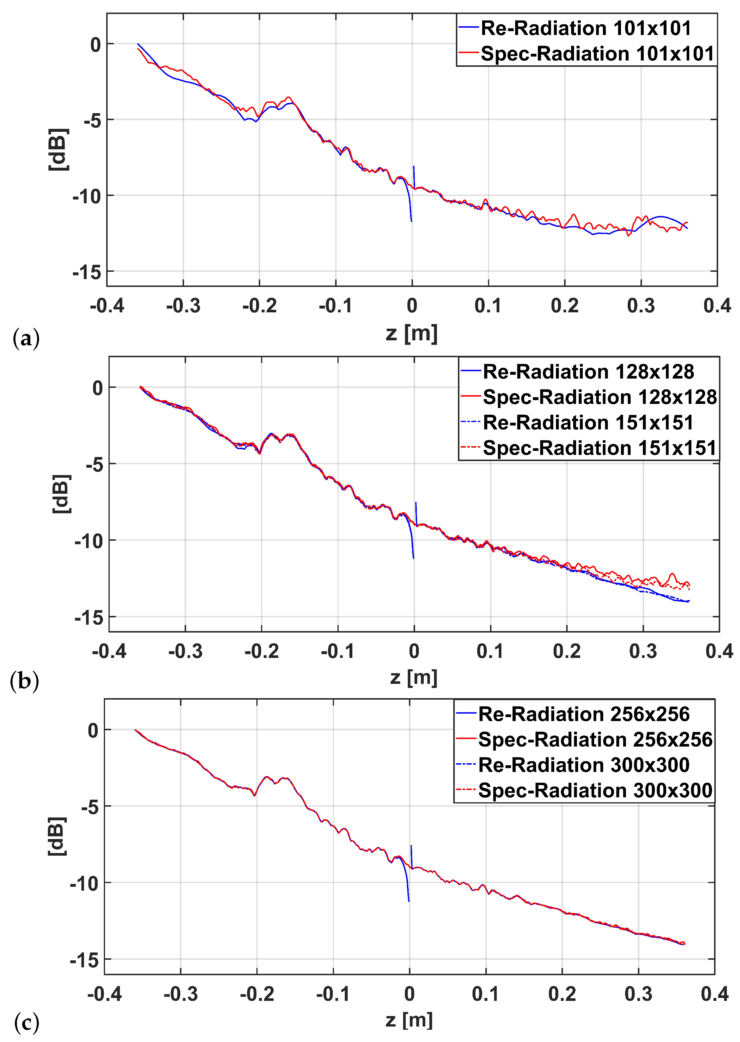
3.2. Influence of the Grid Point Distance

For the efficiency of non-destructive testing with air-coupled ultrasound (ACU), the measurement point distance in the experiment is also an important parameter. The more measurement points are required, the more time for the data acquisition or more equipment (e.g., more receivers) is needed. Using the measurement with the ø20 mm flaw imitate, the influences of the grid point distance is investigated for both the re-radiation method and the spec-radiation method. Here, and for further investigations, the measurement window size is constant at approximately 200 mm × 200 mm, and the evaluation window size is approximately 2.5 times larger, due to zero-padding. Only the grid point distance dx and dy will change. In order to get a good comparison with the re-radiation method, the amplitude distribution on the surface of the particleboard is first calculated and displayed for different grid point distances using the re-radiation method. Figure 13a depicts this for the 2 mm grid. As expected, this is optically identical to the result of the spec-radiation method in Figure 12 from Section 3.1, with a grid point distance of 2 mm. There are artifacts in the corners that can be misinterpreted as another sound source and thus complicate the evaluation with a 8 mm grid point distance (see Figure 13b). However, if the approximate position of the transmitter is known, the flaw is still detectable. With a grid point distance of 12 mm, these errors occur at a higher rate and are closer to the evaluation area (see Figure 14a). However, with knowledge of the approximate range in which the transmitter is located, the flaw can still be identified since a separation from the artifacts is possible. From a grid point distance of 16 mm, the artifacts are so close to the evaluation area that it is no longer possible to ignore them (see Figure 14b). The flaw can at most be identified by exact knowledge of its position, everything else would be an estimation. When calculating the same situations with the spec-radiation method, these artifacts do not occur.

Figure 15a depicts the result for a grid point distance of 8 mm calculated by the spec-radiation method. The transmitter and the flaw can be seen clearly. There are no artifacts that could be mistaken for sound sources. Even with a grid point distance of 12 mm, both the transmitter and the flaw are still clearly visible (see Figure 15b). In the area of the flaw, however, it is noticeable that the amplitude drop is not as strong and, therefore, only a yellowish coloring and no blue coloring appears. While the re-radiation method identifies the ø20 mm flaw with a grid point distance of 16 mm (see Figure 14b) through guessing or by exact knowledge of the position of the flaw, the spec-radiation method identifies both the transmitter and the flaw unambiguously (see Figure 16a). At a grid point distance of 18 mm, the flaw can no longer be identified (see Figure 16b). The transmitter and its position can still be identified. These results show that the spec-radiation method gives clearer results than the re-radiation method using rough measurement grids. The extent to which the results with large grid point distances can be improved and thus increase the detectability of flaws with the spec-radiation method using the technique from Schmelt et al. [22], as with the re-radiation method, is examined in the following Section 3.3.

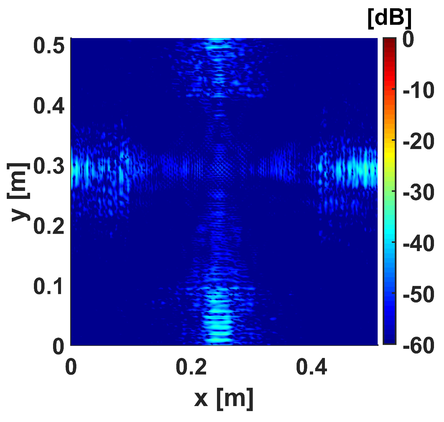
3.3. Results with Enhancement of the Detectability

For the re-radiation method, it has already been shown in [22] that from the data used here, a grid point distance of dx = dy = 18 mm is sufficient to identify the ø20 mm flaw if the time data of the measurement are interpolated to a finer grid before processing. The resulting new grid then contains the measured points and interpolated points. This results in a virtual grid point distance that is smaller than the one originally used for the measurement. In [22], the grid point distance was changed from 18 mm to 2 mm. The command “interp3” with the “spline” interpolation in the program Matlab was identified as a good compromise in effort and accuracy. The same refinement method has been applied to the data from Figure 16b. The sound pressure field is reconstructed by the spec-radiation method, depicted in Figure 17. This shows that the refinement method can be applied here as well. The evaluated data allow a clear identification of the flaw, unlike in Figure 16b. This is expected, since the re-radiation method also produces positives results for this grid point distance with a virtual grid point distance of 2 mm. This is because the calculation methods were not changed and the time data was interpolated before processing. This describes a situation similar to Section 3.1, where the input data and the calculation window are large enough and identical.

3.4. Determination of the Computing Speed

To compare the speed and efficiency of the spec-radtiation method compared to the re-radiation method in the numerical calculation obtained using the process shown in Figure 3, an idealized circular piston transducer was investigated. The amplitude distribution in the plane is depicted in Figure 18. In the red area, the amplitude is 1, and in the blue area the amplitude is 0. The signal is a pulse of two 50 kHz sinusoidal waves and the grid point distance is 2 mm. The surrounding medium was air. The propagation was calculated up to a distance of 1 m in increments of 1 mm, which requires the calculation of 1000 planes. In Figure 19, the amplitude distributions of the two calculations are given. These look almost identical. Differences only become prominent when the scaling is extended to −60 dB (see Figure 20). The larger differences become visible especially at the borders. During the re-radiation method, it appears as if sound enters the volume from the sides and the sound from the piston transducer cannot spread uninhibitedly to the sides. This is not the case with spec-radiation. Corresponding to the pole point of the re-radiation method described in Section 3.1 (see Figure 7), it does not give the default values in layer 0, whereas the spec-radiation method reproduces this exactly.

For the calculation, a standard computer was used with a processor of the type: Intel(R) Core(TM) i5-6500 CPU @ 3.2GHz with 32GB RAM and a 64 bit operating system with Windows 10 Pro. The calculation of the 1000 planes with the re-radiation method needed a time of 141 s and the calculation with the spec-radiation method needed 16.6 s. The spec-radiation method took about 12% of the time compared to the re-radiation method. To visualize the result from the spec-radiation method, we produced the Video Supplementary Materials S2, where the amplitude distribution of each plane can be seen in 3D space. Therefore, the spec-radiation method is faster and more accurate than the re-radiation method in calculation.

4. Discussion

In this paper, a new innovative method called spec-radiation for the detection of flaws in wooden particleboards was presented and evaluated. With this method, flaws near the theoretical resolution limit of $\lambda /2$ can be identified. We showed in the analytical derivation that the re-radiation method can be easily interpreted by its representation with spatial coordinates, but requires a lot of computational effort. While the spec-radiation method is more complicated to interpret by using the spatial angular frequency coordinates, it is much more efficient to compute. A comparison of the two methods showed that the spec-radiation method can be 88% faster in computation than the re-radiation method. We showed this using an example of an idealized circular piston transmitter. We also showed that the re-radiation method is less accurate than the spec-radiation method, especially in the peripheral areas (see Figure 20). Another important aspect when it comes to time efficiency is the number of measuring points needed. We showed that with the re-radiation method, it is possible to identify the flaw up to a certain grid point distance, but that there are artifacts that make the interpretation less clear (see Figure 13 and Figure 14). In order to get good interpretable results with the re-radiation method despite a large grid point distance, one has to rely on techniques, as in Schmelt et al. [22]. For the spec-radiation method, it was shown that a large grid point distance does not produce the same artifacts as with the re-radiation method and that a ø20 mm flaw can still be clearly identified with a 16 mm grid point distance. For even larger grid point distances, we showed that the technique from Schmelt et al. [22] can also be used to increase detectability. We also showed that the re-radiation method has a pole near the measuring plane, which makes the calculation results inaccurate close to the measurement plane. This pole position does not exist in the spec-radiation method and at the position of the measuring plane exactly the measuring plane is returned. With the help of the attached videos, we showed that we can determine and interpret the amplitude sound fields in space as well as the transient sound fields with the spec-radiation method. We are confident that this is a big step towards real-time analysis in the non-destructive air-coupled ultrasonic testing of wood-based materials.

References

1. Sokolov, S.Y. On the problem of the propagation of ultrasonic oscillations in various bodies. Elek. Nachr. Tech. 1929, 6, 454–460. [Google Scholar]
2. Schafer, M. The Effect of Experimental Conditions on Acousto-Ultrasonic Reproducibility. IEEE Ultrason. Symp. 2000, 771–778. [Google Scholar] [CrossRef]
3. Gyekenyesi, A.L.; Harmon, L.M.; Kautz, H.E. The Effect of Experimental Conditions on Acousto-Ultrasonic Reproducibility. In Proceedings of the Nondestructive Evaluation and Health Monitoring of Aerospace Materials and Civil Infrastructures SPIE, San Diego, CA, USA, 18 June 2002; Volume 4704, pp. 177–186. [Google Scholar] [CrossRef]
4. Fang, Y.; Lin, L.; Feng, H.; Lu, Z.; Emms, G.W. Review of the use of air-coupled ultrasonic technologies for nondestructive testing of wood and wood products. Comput. Electron. Agric. 2017, 137, 79–87. [Google Scholar] [CrossRef]
5. Zhang, Y.; Sidibé, Y.; Maze, G.; Leon, F.; Druaux, F.; Lefebvre, D. Detection of damages in underwater metal plate using acoustic inverse scattering and image processing methods. Appl. Acoust. 2016, 103, 110–121. [Google Scholar] [CrossRef]
6. Jasiuniene, E.; Raisutis, R.; Sliteris, R.; Voleiis, A.; Jakas, M. Ultrasonic NDT of wind turbine blades using contact pulse-echo immersion testing with moving water container. Ultragarsas J. 2008, 63, 28–32. [Google Scholar]
7. Mitri, F.G.; Greenleaf, J.F.; Fatemi, M. Comparison of continuous-wave (CW) and tone-burst (TB) excitation modes in vibro-acoustography: Application for the non-destructive imaging of flaws. Appl. Acoust. 2009, 70, 333–336. [Google Scholar] [CrossRef]
8. Sanabria, S.; Mueller, C.; Neuenschwander, J.; Niemz, P.; Sennhauser, U. Air-coupled ultrasound as an accurate and reproducible method for bonding assessment of glued timber. Wood Sci. Technol. 2011, 45, 645–659. [Google Scholar] [CrossRef] [Green Version]
9. Hillger, W.; Bühling, L.; Ilse, D. Review of 30 Years Ultrasonic Systems and Developments for the Future. CNDT2014. Available online: https://www.ndt.net/search/docs.php3?id=16725 (accessed on 2 September 2020).
10. Chimenti, D.E. Review of air-coupled ultrasonic materials characterization. Ultrasonics 2014, 54, 1804–1816. [Google Scholar] [CrossRef]
11. Álvarez Arenas, T.E.G. Acoustic Impedance Matching of Piezoelectric Transducers to the Air. IEEE Trans. Ultrason. Ferroelectr. Freq. Control 2014, 51, 624–633. [Google Scholar] [CrossRef]
12. Dunky, D.; Niemz, P. Holzwerkstoffe und Leime; Springer: Berlin/Heidelberg, Germangy, 2002. [Google Scholar] [CrossRef]
13. Niemz, P. Bestimmung von Fehlverklebungen mittels Schallaufzeitmessung. Holz Als Roh Und Werkst. 1995, 53, 236. [Google Scholar] [CrossRef]
14. Bucur, V.; Böhnke, I. Factors affecting ultrasonic measurements in solid wood. Ultrasonics 1994, 32, 385–390. [Google Scholar] [CrossRef]
15. Döring, D. Air-Coupled Ultrasound and Guided Acoustic Waves for Application in Non-Destructive Material Testing; OPUS: Stuttgart, Germany, 2011. [Google Scholar] [CrossRef]
16. Laybed, Y.; Huang, L. Ultrasound time-reversal MUSIC imaging with diffraction and attenuation compensation. IEEE Trans. Ultrason. Ferroelectr. Freq. Control 2012, 59, 2186–2200. [Google Scholar] [CrossRef] [PubMed]
17. Singh, V. Acoustical imaging techniques for bone studies. Appl. Acoust. 1989, 27, 119–128. [Google Scholar] [CrossRef]
18. Sanabria, S.; Marhenke, T.; Furrer, R.; Neuenschwander, J. Calculation of volumetric sound field of pulsed air-coupled ultrasound transducers based on single-plane measurements. IEEE Trans. Ultrason. Ferroelectr. Freq. Control 2018, 65, 72–84. [Google Scholar] [CrossRef]
19. Marhenke, T.; Neuenschwander, J.; Furrer, R.; Zolliker, P.; Twiefel, J.; Hasener, J.; Wallaschek, J.; Sanabria, S. Air-coupled ultrasound time reversal (ACU-TR) for subwavelength non-destructive imaging. IEEE Trans. Ultrason. Ferroelectr. Freq. Control 2020, 67, 651–663. [Google Scholar] [CrossRef]
20. Marhenke, T.; Sanabria, S.; Chintada, B.; Furrer, R.; Neuenschwander, J.; Goksel, O. Acoustic field characterization of medical array transducers based on unfocused transmits and single-plane hydrophone measurements. Sensors 2019, 19, 863. [Google Scholar] [CrossRef] [Green Version]
21. Marhenke, T.; Sanabria, S.; Twiefel, J.; Furrer, R.; Neuenschwander, J.; Wallaschek, J. Three dimensional sound field computation and optimization of the delamination detection based on the re-radiation. In Proceedings of the 12th European Conference on Non-destructive Testing (12th ECNDT), Gothenburg, Sweden, 11–15 June 2018. [Google Scholar]
22. Schmelt, A.; Marhenke, T.; Hasener, J.; Twiefel, J. Investigation and Enhancement of the Detectability of Flaws with a Coarse Measuring Grid and Air Coupled Ultrasound for NDT of Panel Materials Using the Re-Radiation Method. Appl. Sci. 2020, 10, 1155. [Google Scholar] [CrossRef] [Green Version]
23. Schmelt, A.; Li, Z.; Marhenke, T.; Twiefel, J. Aussagefähigkeit von Fehlstellenimitaten in der ZfP. In Daga2020; University of Oldenburg: Oldenburg, Germany, 2020; pp. 1133–1136. ISBN 978-3-939296-17-1. [Google Scholar]
24. Tsysar, S.; Sapozhnikov, O. Ultrasonic holography of 3D objects. In Proceedings of the IEEE International Ultrasonics Symposium, Rome, Italy, 20–23 September 2009; pp. 737–740. [Google Scholar] [CrossRef]
25. Schmelt, A.; Marhenke, T.; Twiefel, J. Identifying objects in a 2D-space utilizing a novel combination of a re-radiation based method and of a difference-image-method. In Proceedings of the 23rd International Congress on Acoustics (ICA 2019), Aachen, Germany, 9–13 September 2019; ISBN 978-3-939296-15-7. [Google Scholar]
26. Delen, N.; Hooker, B. Free-space beam propagation between arbitrarily oriented planes based on full diffraction theory: A fast Fourier transform approach. J. Opt. Soc. Am. A 1998, 15, 857–867. [Google Scholar] [CrossRef]
27. Booker, H.G.; Clemmow, P.C. The concept of an angular spectrum of plane waves, and its relation to that of polar diagram and aperture distribution. Proc. IEEE Part III Radio Commun. Eng. 1950, 97, 11–17. [Google Scholar] [CrossRef] [Green Version]
28. Ratcliffe, J.A. Some Aspects of Diffraction Theory and their Application to the Ionosphere. Rep. Prog. Phys. 1956, 19, 188–267. [Google Scholar] [CrossRef]
29. Boyer, A.L.; Hirsch, P.M.; Jordan, J.A.; Lesem, L.B.; Van Rooy, D.L. Reconstruction of tultrasonic images by backward propagation. Proc. Acoust. Hologr. 1970, 3, 333–348. [Google Scholar] [CrossRef]
30. Schafer, M.E.; Lewin, P.A. Transducer characterization using the angular spectrum method. J. Acoust. Soc. Am. 1989, 85, 2202–2214. [Google Scholar] [CrossRef]
31. De Belleval, J.F.; Messaoud-Nacer, N. Ultrasonic transducer beams model, using transient angular spectrum. Rev. Prog. Quant. Nondestruct. Eval. 1999, 18, 1101–1106. [Google Scholar] [CrossRef]
32. McGough, R.J.; Samulski, T.; Kelly, J. An efficient grid sectoring method for calculations of the near-field pressure generated by a circular piston. J. Acoust. Soc. Am. 2004, 115, 1942–1954. [Google Scholar] [CrossRef] [PubMed]
33. Zeng, X.J.; McGough, R.J. Evaluation of the angular spectrum approach for simulations of near-field pressures. J. Acoust. Soc. Am. 2008, 123, 68–76. [Google Scholar] [CrossRef] [PubMed]
34. Alles, E.J.; Zhu, Y.; van Dongen, K.W.A.; McGough, R.J. Rapid Transient Pressure Field Computations in the Nearfield of Circular Transducers Using Frequency-Domain Time-Space Decomposition. Ultrason. Imaging 2012, 34, 237–260. [Google Scholar] [CrossRef] [Green Version]
35. Yan, X.; Hamilton, M.F. Angular Spectrum Decomposition Analysis of Second Harmonic Ultrasound Propagation and Its Relation to Tissue Harmonic Imaging. In Proceedings of the 4th International Workshop on Ultrasonic and Advanced Methods for Nondestructive Testing and Material Characterization, North Dartmouth, MA, USA, 19 June 2006; pp. 155–168. [Google Scholar]
36. Peng, H.; Lu, J.; Han, X. High frame rate ultrasonic imaging system based on the angular spectrum principle. Ultrasonics 2006, 44, e97–e99. [Google Scholar] [CrossRef]
37. Aanes, M.; Lohne, K.D.; Lunde, P.; Vestrheim, M. Ultrasonic beam transmission through a water-immersed plate at oblique incidence using a piezoelectric source transducer. Finite element-angular spectrum modeling and measurements. In Proceedings of the 2012 IEEE International Ultrasonics Symposium, Dresden, Germany, 7–10 October 2012; pp. 1972–1977. [Google Scholar] [CrossRef]
38. Liu, D.L.; Waag, R.C. Propagation and backpropagation for ultrasonic wavefront design. IEEE Trans. Ultrason. Ferroelectr. Freq. Control 1997, 44, 1–13. [Google Scholar] [CrossRef]
39. Jakevičius, L.; Demčenko, A. Ultrasound attenuation dependence on air temperature in closed chambers. Ultrasound 2008, 63, 1942–1954. [Google Scholar]
40. Stößel. Air-Coupled Ultrasound Inspection as a New Non-Destructive Testing Tool for Quality Assurance; OPUS: Stuttgart, Germany, 2004. [Google Scholar] [CrossRef]
41. Goodman, J.W. Introduction to Fourier Optics; W. H. Freeman and Company: New York, NY, USA, 2017. [Google Scholar]
42. Schmerr, L.; Song, S.J. Ultrasonic Nondestructive Evaluation Systems; Springer: Boston, MA, USA; New York, NY, USA, 2007. [Google Scholar] [CrossRef]
43. Sommerfeld, A. Optics: Lectures on Theoretical Physics; Academic: New York, NY, USA, 1964. [Google Scholar]
44. Sommerfeld, A. Über die Ausbreitung der Wellen in der drahtlosen Telegraphie. An. Der Phys. 1909, 4, 665–736. [Google Scholar] [CrossRef] [Green Version]
45. Krautkrämer, J.; Krautkrämer, H. Werkstoffprüfung mit Ultraschall; Springer: Berlin/Heidelberg, Germany, 1980. [Google Scholar] [CrossRef]
46. Fahr, A. Aeronautical Applications of Non-Destructive Testing; DEStech Publications, Inc.: Lancaster, PA, USA, 2014. [Google Scholar]
47. Cramer, O. The variation of the specific heat ratio and the speed of sound in air with temperature, pressure, humidity, and CO2 concentration. J. Acoust. Soc. Am. 1993, 93, 2510–2516. [Google Scholar] [CrossRef]
48. Conta, S.; Santoni, A.; Homb, A. Benchmarking the vibration velocity-based measurement methods to determine the radiated sound power from floor elements under impact excitation. Appl. Acoust. 2020, 107457. [Google Scholar] [CrossRef]
49. Wolf, E. Three-dimensional structure determination of semi-transparent objects from holographic data. Opt. Commun. 1969, 1, 153–156. [Google Scholar] [CrossRef]
50. Simonetti, F. Multiple scattering: The key to unravel the subwavelength world from the far-field pattern of a scattered wave. Phys. Rev. 2006, 73. [Google Scholar] [CrossRef] [PubMed]
Figure 1. Experimental setup with a flaw imitation at the top of the wooden particleboard. NI = National Instruments, Schmelt et al. [22].
Applsci 10 06663 g001
Figure 2. Flow chart for the practical realization of the spec-radiation and re-radiation technique.
Applsci 10 06663 g002
Figure 3. Flow chart of the flow chart block of the radiation technique (see Figure 2) for the practical realization of the spec-radiation and re-radiation technique.
Applsci 10 06663 g003
Figure 4. Amplitude (a) and angle (b) at the top of the wooden particleboard without a flaw. Evaluated with the spec-radiation method for the frequency 50kHz, with dx = dy = 2 mm and a grid of the size 101 × 101 points.
Applsci 10 06663 g004
Figure 5. Amplitude (a) and angle (b) at the top of the wooden particleboard without a flaw. Evaluated with the re-radiation method for the frequency 50kHz, with dx = dy = 2 mm and a grid of the size 101 × 101 points.
Applsci 10 06663 g005
Figure 6. Difference image D I of the amplitudes of the back propagated sound field of the spec- and re-radiation method.
Applsci 10 06663 g006
Figure 7. Maximum value of several calculated planes using the re-radiation method for calculation (blue) and with the spec-radiation method for calculation (red). For the grid of the size 101 × 101 points (a), for the grid of the size 128 × 128 points and for the grid of the size 151 × 151 points (b) and for the grid of the size 256 × 256 points and for the grid of the size 300 × 300 points (c).
Applsci 10 06663 g007
Figure 8. Amplitude (a) and angle (b) at the top of the wooden particleboard without a flaw. Evaluated with the spec-radiation method for the frequency 50kHz, with dx = dy = 2 mm and a grid of the size 256 × 256 points.
Applsci 10 06663 g008
Figure 9. Amplitude (a) and angle (b) at the top of the wooden particleboard without a flaw. Evaluated with the re-radiation method for the frequency 50kHz, with dx = dy = 2 mm and a grid of the size 256 × 256 points.
Applsci 10 06663 g009
Figure 10. Difference image D I of the amplitudes of the back propagated sound field of the spec- and re-radiation method with an evaluation window size of 256 × 256 point.
Applsci 10 06663 g010
Figure 11. Amplitude at the top of the wooden particleboard with a ø4 mm piece of paper. Evaluated with the spec-radiation method for the frequency 50 kHz, with dx = dy = 2 mm and a grid of the size 256 × 256 points.
Applsci 10 06663 g011
Figure 12. Amplitude at the top of the wooden particleboard with a ø20 mm piece of paper. Evaluated with the spec-radiation method for the frequency 50 kHz, with dx = dy = 2 mm and a grid of the size 256 × 256 points.
Applsci 10 06663 g012
Figure 13. Amplitude at the top of the wooden particleboard with a ø20 mm piece of paper. Evaluated with the re-radiation method for the frequency 48–52 kHz, with (a) dx = dy = 2 mm and (b) dx = dy = 8 mm a grid of the size 512 mm × 512 mm.
Applsci 10 06663 g013
Figure 14. Amplitude at the top of the wooden particleboard with a ø20 mm piece of paper. Evaluated with the re-radiation method for the frequency 48–52 kHz, with (a) dx = dy = 12 mm and (b) dx = dy = 16 mm a grid of the size 512 mm × 512 mm.
Applsci 10 06663 g014
Figure 15. Amplitude at the top of the wooden particleboard with a ø20 mm piece of paper. Evaluated with the spec-radiation method, for the frequency 48–52 kHz, with (a) dx=dy=8 mm and (b) dx = dy = 12 mm and a grid of the size 512 mm × 512 mm.
Applsci 10 06663 g015
Figure 16. Amplitude at the top of the wooden particleboard with a ø20 mm piece of paper. Evaluated with the spec-radiation method, for the frequency 48–52 kHz, with (a) dx = dy = 16 mm and (b) dx = dy = 18 mm and a grid of the size 512 mm × 512 mm.
Applsci 10 06663 g016
Figure 17. Amplitude at the top of the wooden particleboard with a ø20 mm piece of paper. Evaluated with the spec-radiation method, for the frequency 48–52 kHz, with an original grid point distance of dx = dy = 18 mm enhancet to d x V i r t = d y V i r t = 2 mm and a grid of the size 512 mm × 512 mm.
Applsci 10 06663 g017
Figure 18. Amplitude distribution of the idealized circular piston transducer.
Applsci 10 06663 g018
Figure 19. Amplitude distribution of the idealized circular piston transducer after forward propagation with the (a) spec-radiation method and (b) the re-radiation method. Normalized to the maximum in the volume.
Applsci 10 06663 g019
Figure 20. Amplitude distribution of the idealized circular piston transducer after forward propagation with the (a) spec-radiation method and (b) the re-radiation method. Normalized to the maximum in the volume. Scaled to −60 dB.
Applsci 10 06663 g020