Intersection Routing Based on Fuzzy Multi-Factor Decision for VANETs

Abstract

Vehicular ad hoc network (VANET) is a special form of mobile ad hoc network (MANET), which plays a key role in the intelligent transportation system (ITS). Though many outstanding geographic routing protocols are designed for VANETs, a majority of them use parameters that only affect routing performance. In this article, we propose an intersection routing based on fuzzy multi-factor decision (IRFMFD), which utilizes several features. The scheme is divided into two parts, namely vehicular decision management and intersection decision management. In the vehicular component, candidate vehicles between two static nodes (SNs) located at two intersections derive potential routing paths considering distance, neighbor quantity, and relative velocity. In the intersection component, the candidate SN was chosen from the current intersection’s 2-hop neighbors which were connected with the current intersection by a route that was decided on in part one. To get the best scheme, we also introduced other factors to estimate the number of hops in each link and link lifetime. The simulation shows that the IRFMFD outperforms on delivery ratio and end-to-end delay compared with AODV (Ad hoc on-demand distance vector), GPSR (Greedy perimeter stateless routing) and GeOpps (Geographical opportunistic routing).

1. Introduction

The rapid increase in the number of vehicles and advancements in mobile internet has drawn the attention of experts in academia and industry towards vehicular ad-hoc networks (VANETs). VANET is a special kind of mobile ad-hoc networks (MANETs), where vehicles are the main communication participants [1,2]. VANET system communication is in two forms, namely vehicle-to-vehicle (V2V) and vehicle-to-infrastructure (V2I). In contrast to MANETs, VANETs are characterized by high mobility. Hence, the network topology of VANETs changes continuously. As a result of vehicular movements, communication link conditions among vehicles vary frequently, influencing intermittent network disconnection. Nevertheless, mobility of vehicles is predictable through GPS indicators, such as obstacles on both sides of the road segment, vehicle position, and speed [3].

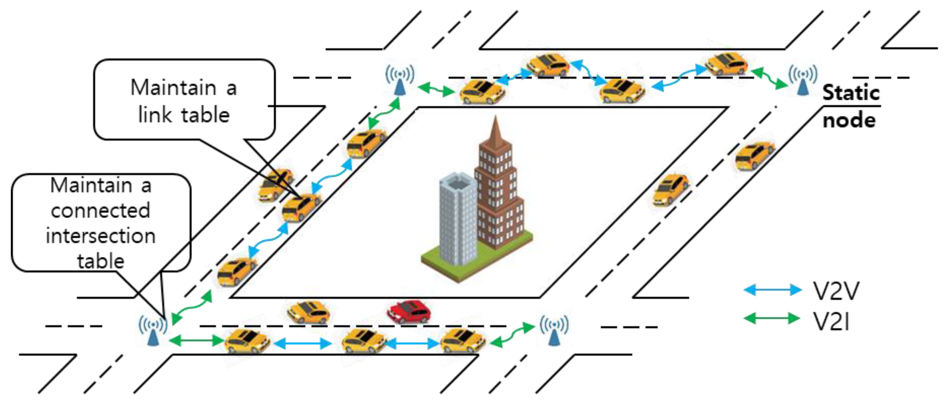
Owing to the characteristics of VANETs, designing a suitable routing protocol remains challenging due to the requirement of a high delivery ratio at the final destination within a short time [4,5]. In VANETs, data packets are transferred along road segments and routing decisions are made at intersections. Hence, if a link breaks, the packet will be retransferred to the last intersection node to determine another potential route. Hence, SNs at intersections analyze connection information of adjacent SNs to guarantee connectedness. Accordingly, vehicles select potential road segments to forward data packets. Selecting a vehicle from the candidate vehicles as the next hop between two SNs remains a key challenge to be addressed.

Herein we propose a routing protocol for VANETs that derives two types of decisions, namely vehicle decision and intersection decision. Vehicles between two SNs at two intersections derive vehicle decisions. (1) Candidate vehicles are selected by analyzing three vehicle factors. A fuzzy performance score is calculated for each candidate based on the fuzzy factor score and their real-time weights. Finally, a link decision between two SNs can be made by candidates with the highest performance score. Every vehicle in the link will keep the complete link information when the link path discovery finishes between two intersections. (2) The candidate SNs are chosen from the current vehicle’s 2-hop neighbors who are connected with the current vehicle by a route that is decided in vehicle decision. Every SN also keeps a table on connected SNs at the intersection. Figure 1 shows the architecture of this paper. The simulation shows that the IRFMFD outperforms on delivery ratio and end-to-end delay compared with AODV, GPSR and GeOpps.

The rest of this paper is organized as follows: in Section 2, we discuss the related works; in Section 3, the details of the routing protocol we proposed are described; in Section 4, the simulation results are shown; in Section 5, we discuss the simulation results and our future work; and finally, in Section 6, this paper is concluded.

2. Related Work

In this section, we review some existing routing protocols to indicate our motivations.

This section describes the unicast routing protocols in which a single data packet is transported to the destination vehicle without any duplication due to the overhead concern. There are two categories of routing protocols: topology-based routing protocols and geographic (position-based) routing protocols [6,7].

In topology-based routing protocols, the links’ information that exists in the network is used to perform packet forwarding. They can also further be divided into proactive and reactive routing. The distinct feature of proactive routing is that the full routing information such as the next forwarding hop is maintained in the background regardless of communication requests. In reactive routing, a route will be established only when a vehicle must communicate with another vehicle.

The two more famous topology-based routing protocols are ad hoc on-demand distance vector (AODV) [8] and the dynamic source routing (DSR) [9]. These two routing protocols maintain only current route information to reduce packet overhead. Nevertheless, increasing overhead size is inevitable with increasing network diameter results from vehicle mobility.

Geographic routing (GR) determines forwarding route considering destination position and the positions of the vehicle’s 1-hop neighbors. Vehicles that are within a vehicle’s radio range will become neighbors of the vehicle. Geographic routing assumes that not only every vehicle knows its position, but also the sending vehicle knows the receiving vehicle’s position by the global positioning system (GPS) unit. Since GR neither exchanges link state information nor maintains established routes as topology-based routing protocols, it is more robust and promising compared with VANETs which are highly dynamic.

GR can be sub-classified into three categories, namely non-delay tolerant network (non-DTN), delay tolerant network (DTN), and hybrid [10]. DTN considers dysconnectivity, whereas non-DTN does not consider intermittent connectivity and is suitable for densely populated VANETs. Hybrid combines non-DTN and DTN routing protocols to exploit partial network connectivity. The key objective of non-DTN is to minimize packet delivery time from source to destination. Greedy forwarding is the commonly used technique in which the fundamental principle is to forward packets to a neighbor, which is geographically closer to the destination. However, the local maximum issue could appear when a vehicle reaches closer to the destination and finds no neighbors closer to the destination than the vehicle itself.

Greedy perimeter stateless routing (GPSR) [11] is the most well-known geographic routing protocol in VANETs. A vehicle forwards a packet to a 1-hop neighbor which is geographically closest to the destination vehicle. This mode is called greedy mode, and a recovery mode is switched to when a packet reaches the local maximum. The packet is forwarded along the perimeter of a planar graph without crossing edges based on the right-hand rule. If the packet reaches a vehicle whose distance to the destination is closer than the vehicle at the local maximum to the destination, the packet resumes forwarding in greedy mode. Greedy perimeter coordinator routing (GPCR) [12] enhances GPSR by using the Dijkstra shortest path algorithm to determine the junctions that have to be traversed based on a static street map. A packet has to be forwarded to a vehicle that is located on the junction because junctions are the only places where routing decisions are made. Packets can be forwarded between the junctions in greedy mode. And GPCR consists of two parts. One is a restricted greedy forwarding procedure and another is a repair strategy that is based on the topology of real-world streets and junctions. Hence, GPCR not only eliminates the inaccuracy of vehicle planarization but also improves routing performance as packets travel shorter hops in the perimeter mode.

More and more researchers proposed protocols considering urban traffic characteristics and intersections. The shortest-path-based traffic-light-aware routing (STAR) protocol [13] considers the status of traffic lights. In STAR, packets are attempted to forward to a connected road segment based on the status of traffic lights. Similarly, the intersection-based connectivity aware routing (iCAR) [14] obtains the road connectivity proactively and decides the next intersections by evaluating the lifetime of a link based on real-time traffic information. However, both STAR and iCAR only consider the traffic conditions of the current road segment and ignore the subsequent routing. The infrastructure-based connectivity aware routing (iCAR-II) [15] not only adopts the intersection-based connectivity-aware routing, but also makes the routing direction based on the global network topology. The strategy of iCAR-II is to construct a global network topology by predicting the network connectivity and update location servers with real-time network information. It then selects the shortest path from source to destination. Though iCAR-II enables multi-hop vehicular application, it also loses packets when roads are disconnected. Furthermore, based on the name of iCAR-II, it is known that iCAR-II is very dependent on infrastructure.

The notable DTN vehicular routing protocols are VADD and GeOpps. In vehicle-assisted data delivery (VADD) [16], each vehicle maintains a matrix of estimated delay based on the information of the distance between intersections and the vehicular density on the road. Then, the routing path is decided by the delay matrix. The enhancement of VADD is called static-vehicle assisted adaptive data distribution protocol in VANETs (SADV) [17] and SNs are employed at intersections to store-and-forward packets in due time.

Geographical opportunistic routing (GeOpps) [18] determines a vehicle which is closer to the destination based on a navigation system. It calculates the shortest distance from the packet’s destination to the nearest point (NP) and estimates the arrival time to the destination. During the travel of vehicles, if there is another vehicle that has a shorter estimated arrival time, the packet will be forwarded to that vehicle. The process repeats until the packet arrives at the destination. The GeOpps was equipped with local infostations at the intersections.

The traffic-aware routing protocol (TAROC) [19] proposed a cooperative collection method. A real-time traffic condition map is drawn by cooperation between information aggregators at intersections and information collectors on road segments, and a data route with a weight score is constructed.

While many geographic routing protocols have been proposed, all of them forward the packets based on the greedy forwarding strategy, which means the packet should be forwarded as far as possible inside the range of communication radio. However, as we know, the biggest characteristic of the VANETs is the high mobility, meaning the link is easily broken. The biggest advantage of the greedy forwarding strategy is that it reduces the hop counts, but the link break rate is increased. The link should be recovered or rebuilt when the link is broken. At that condition, the hop counts must increase and more time must also be spent. Due to the fact that the routing decision is made at the intersection, the packet forwarded should return the last intersection along the road segment and find another route if the link is unconnected between two intersections. Therefore, if the vehicles know the connection status in advance, the vehicles can choose the best segment to forward the packets such that the hop count can be reduced. In addition, most of the existing proposals only consider a single factor, such as velocity. This is another reason why the link is fragile and easy to break.

In recent years, more and more researchers have focused on fuzzy routing protocols. Adaptive fuzzy multiple attribute decision routing (AFMADR) [20] designs an adaptive weight assignment mechanism to calculate weights of four proposed attributes and selects a candidate with the highest fuzzy utility score as the next hop transmission. Fuzzy logic-based directional geographic routing (FL-DGR) [21] proposed the fuzzy logic decision system (FL-DS) which is used for estimating multiple metrics to choose the next hop for forwarding packets. Since the recovery strategy of FL-DGR adopts the carry-and-forward approach, it is a DTN routing protocol, and it will perform well in some conditions where there are few vehicles and links break frequently, such as late at night.

We summarize the characteristics of the representative routing protocols including AODV, GPSR, GeOpps, iCAR, iCAR-II, TAROC, and AFMADR schemes to compare with our proposed scheme as shown in

Table 1. Summary of related routing protocols.

Routing Protocol	Type	Sub-Type	Map-Based	Intersection Based	Traffic Aware
AODV	Topological	Reactive	No	No	No
GPSR	Geographic	Non-DTN	No	No	No
GeOpps	Geographic	DTN	Yes	No	No
iCAR	Geographic	Non-DTN	Yes	Yes	Yes
iCAR-II	Geographic	Non-DTN	Yes	Yes	Yes
TAROC	Geographic	Non-DTN	Yes	Yes	Yes
AFMADR	Geographic	Non-DTN	Yes	Yes	Yes
FL-DGR	Geographic	DTN	Yes	No	Yes
IRFMFD	Geographic	Non-DTN	Yes	Yes	Yes

.

3. Intersection Routing Based on Fuzzy Multi-Factor Decision

In this section, the proposed routing protocol is discussed in detail. The proposed protocol is further divided into two parts: (1) vehicle decision and (2) intersection decision. In the vehicle decision, the routing is performed based on the vehicle routing between two adjacent SNs. However, in the intersection decision, the routing is decided based on the SN routing.

3.1. System Components

In this paper, we suppose the vehicles and SNs have the following features:

• Vehicles and SNs are equipped with a GPS receiver and a digital map. A wireless transceiver also exists and the transmission coverage of SNs can cover the area of the intersections.
• Each vehicle maintains a neighbor table to record the information about other vehicles based on the beacon messages they received.

  Table 2. Beacon message.

  ID

  Position Vector

  Velocity Vector

  Neighbor Quantity

  Road ID

  Source Intersection ID

  Target Intersection ID

  Link Sequence

  Lifetime

  shows the format of the beacon message. The link sequence maintains the information about the reverse route to the source intersection node. The lifetime is the minimum time between two vehicles in the link path.
• Each SN also maintains a neighbor table to record the information of its neighbors within 2-hop.

  Table 3. Static node neighbor table.

  Node ID	Position	1-Hop	2-Hop	Joint Node	Road ID	Link Sequence	Vehicle Quantity	Lifetime
  a b -	$({\mathrm{X}}_a,{\mathrm{Y}}_a)$ $({\mathrm{X}}_b,{\mathrm{Y}}_b)$ -	Yes No -	No Yes -	- a -	- - -	- - -	${\mathrm{n}}_a$ ${\mathrm{n}}_b$ -	${\mathrm{t}}_a$ ${\mathrm{t}}_b$ -

  shows the format of an SN neighbor table. Assume the SN is $S{N}_c$. Then, $S{N}_a$ is its 1-hop neighbor and $S{N}_b$ is its 2-hop neighbor. $S{N}_a$ is the joint node between $S{N}_c$ and $S{N}_b$. Vehicle quantity $n_b$ is the sum of vehicles in links from $S{N}_c$ to $S{N}_b$. Lifetime $t_b$ is the minimum time between $lin{k}_{ac}$ (the link between $S{N}_c$ and $S{N}_a$) and $lin{k}_{ab}$ (the link between $S{N}_a$ and $S{N}_b$).

3.2. Vehicle Decision

The routing protocols in VANETs presented in the current literature depends on a certain number of factors. Therefore, to follow a standard nomenclature for the characterization, we consider three key factors as follows:

• Distance: between the current vehicle and the candidate vehicle;
• Neighbor quantity: the number of candidate vehicles’ neighbors;
• Relative velocity: between the current vehicle and the candidate vehicle.

To quantify the three factors, we select a nine-point fuzzy scale system. The fuzzy number is put forward as a triangular fuzzy number (TFN), denoted as follows [22]:

$$\tilde{\mathrm{A}}=\left(\mathrm{l},\mathrm{m},\mathrm{u}\right),$$

(1)

where $\mathrm{l}$ and $\mathrm{u}$ are the lower and upper bounds of the fuzzy number $\tilde{\mathrm{A}}$ respectively, and $\mathrm{m}$ is the modal value. In this paper, we assigned four values to the linguistic variable as presented in

Table 4. Triangular fuzzy number.

Linguistic Variable	Triangular Fuzzy Number
Lower	$\tilde{2}=\left(1,2,3\right)$
Low	$\tilde{4}=\left(3,4,5\right)$
High	$\tilde{6}=\left(5,6,7\right)$
Higher	$\tilde{8}=\left(7,8,9\right)$

.

Next, we will illustrate the details on how to evaluate the candidate factors.

3.2.1. Distance

On the premise of receiving the entire message, it is obvious that the best next hop is the vehicle that is farthest away from the current vehicle. Thus, to ensure the integrity of the message forwarded, we divided the radio range into five groups. Further, we evaluated the distance factor of a vehicle with a score D based on different places where the vehicle is located. The farther away from the current vehicle, the higher the score evaluated as presented previously. The fuzzy number D of the distance factor is shown in the following formula:

$$D=\{\begin{array}{ll}\tilde{2},& if 0< distanc\le \frac{1}{4}r\\ \tilde{4},& if \frac{1}{4}r<distance\le \frac{1}{2}r\\ \tilde{6},& if \frac{1}{4}r<distance\le \frac{3}{4}r\\ \tilde{8},& if \frac{3}{4}r<distance\le r\end{array}$$

(2)

where r represents the radio radius.

3.2.2. Neighbor Quantity

Collisions may be introduced if there are many neighboring vehicles around the current vehicle. Also, the current vehicle can choose a much better neighbor as next-hop from these candidates to keep the routing connectivity. As presented previously [23], the road is crowded when the traffic flow reaches 133 vehicles/km/lane. However, in a common urban scenario, the vehicle speed is less than 70 km/h, and the vehicle density is about 20 vehicles/km/lane. We assume that the range of the radio is 250 m and the message can be forwarded within 200 m. We set the period of communication information from an SN to be less than 1 s. In such situations, we can calculate the density within a 6 vehicle/km/lane. In most situations, there is more than one lane on the road, thus we assume the fuzzy number of density factors using the following formula:

$$\mathrm{N}=\{\begin{array}{ll}\tilde{2},& \mathrm{if} \mathrm{neighbors}\le 3\\ \tilde{4},& \mathrm{if} 3<\mathrm{neighbors}\le 6\\ \tilde{6},& \mathrm{if} 6<\mathrm{neighbors}\le 9\\ \tilde{8},& \mathrm{if} \mathrm{neighbors}\ge 10\end{array}$$

(3)

3.2.3. Relative Velocity

The less the relative velocity of two vehicles, the longer the link can be kept between them. The proposed routing protocol keeps the link between two adjacent SNs for some time instead of being used immediately, which preserves the link lifetime for a longer period of time. Also, this not only guarantees the availability of data transmission but can also reduce the collision due to the formation of the link. Suppose the current vehicle speed is $v_0$ and the neighbor vehicle speed is $v_1$. The fuzzy number of the relative velocity between the current vehicle and candidate vehicle is computed with the help of the following equation:

$$\mathrm{V}=\{\begin{array}{ll}\tilde{2},& \mathrm{if}{v}_0\mathrm{and}{v}_1\mathrm{are}\mathrm{in}\mathrm{different}\mathrm{directions}\\ \tilde{4},& \mathrm{if}{v}_0<v_1\\ \tilde{6},& \mathrm{if}{v}_0>v_1\\ \tilde{8},& \mathrm{if}{v}_0=v_1\end{array}$$

(4)

3.2.4. Candidate Vehicle Selection

After the quantification of all three factors, the next step is to calculate the fuzzy performance scores of the potential candidate factors. We defined the set of candidate vehicles as $\mathrm{C}=\left\{C_i\right|i=1,2\dots n\}$, the set of factors as $\mathrm{F}=\left\{F_j\right|j=1,2,3\}$, and weights $\mathrm{W}=\left\{{\tilde{w}}_j\right|j=1,2,3\}$, $\mathrm{X}=\left\{{\tilde{x}}_{ij}\right|i=1,2\dots n;j=1,2,3\}$, which means the jth fuzzy factor score of the ith candidate vehicle based on the factor evaluation of the candidate vehicle as shown above. The fuzzy weights of factors distance, neighbor quantity, and relative velocity are indicated by a TFN, ${\tilde{w}}_j=\left\{l{w}_j,m{w}_j,u{w}_j\right\}$. Here,$l{w}_j$, $m{w}_j$, and $u{w}_j$ stand for the lower, middle, and upper values of the fuzzy weight of the jth factor, respectively.

To depict the differences of the factor scores between vehicles, we import descriptor, the standard deviation of probability theory, and statistics to calculate the weight of these factors. A small variance means that the data points are close to the expected value and each other. Correspondingly, high variance means that the data points are dispersed from the expected value and from each other. In this paper, the standard deviation is used to measure the difference of the same factor between candidate vehicles.

First, the expected value of scores of the jth factor was calculated using the following equation:

$$\widetilde{{\mathrm{r}}_{\mathrm{J}}}\left(\mathrm{x}\right)=\frac{1}{\mathrm{n}}\ast {\sum }_{\mathrm{i}=1}^{\mathrm{n}}\widetilde{{\mathrm{x}}_{\text{IJ}}}$$

(5)

Then, the standard deviation of each factor was calculated as follows:

$$\widetilde{{\mathrm{D}}_{\mathrm{J}}}=\sqrt{\frac{1}{\mathrm{n}}\ast {\sum }_{\mathrm{i}=1}^{\mathrm{n}}{\left[\widetilde{{\mathrm{x}}_{\text{IJ}}}-\widetilde{{\mathrm{r}}_{\mathrm{J}}}\left(\mathrm{x}\right)\right]}^2}$$

(6)

Hence, the weight of each factor was calculated as shown below:

$$\widetilde{{\mathrm{w}}_{\mathrm{J}}}=\widetilde{{\mathrm{D}}_{\mathrm{J}}}/{\displaystyle {\sum }_{\mathrm{j}=1}^3}\widetilde{{\mathrm{D}}_{\mathrm{J}}}$$

(7)

According to the above formulas, the fuzzy performance score and fuzzy relative weight of each factor were obtained and the utility $\widetilde{{\text{u}}_{\text{l}}}$(x) of the ith candidate vehicle can be calculated as follows:

$$\widetilde{{\mathrm{u}}_{\mathrm{I}}}\left(\mathrm{x}\right)={\sum }_{\mathrm{j}=1}^3\widetilde{{\mathrm{x}}_{\text{IJ}}}\ast \widetilde{{\mathrm{w}}_{\mathrm{J}}}$$

(8)

The vehicle with the highest utility will be selected as the next hop:

$$\mathrm{C}=\left\{\widetilde{{\mathrm{u}}_{\mathrm{I}}}\right|\text{max}\widetilde{{\mathrm{u}}_{\mathrm{I}}}\left(\mathrm{x}\right),\mathrm{i}=1,2\dots \mathrm{n}\}$$

(9)

The $\widetilde{{\mathrm{u}}_{\mathrm{I}}}$ is a fuzzy number. However, the non-fuzzy ranking method for fuzzy numbers must be employed to compare the various candidates. The procedure of de-fuzzification involves the location of the best non-fuzzy performance (BNP) value. Generally, several available methods include the mean of maximum, center-of-area (COA), and α-cut method [24]. In this paper, we utilize the center of area (COA) method to determine the best non-fuzzy performance (BNP) [25] value of the candidates. The BNP value for the fuzzy number $\widetilde{{\mathrm{u}}_{\mathrm{l}}}\left(\mathrm{x}\right)$ can be found using the following equation:

$${\mathrm{BNP}}_{\mathrm{i}}=\left[\left({\mathrm{ur}}_{\mathrm{i}}-{\mathrm{lr}}_{\mathrm{i}}\right)+\left({\mathrm{mr}}_{\mathrm{i}}-{\mathrm{lr}}_{\mathrm{i}}\right)\right]/3+{\mathrm{lr}}_{\mathrm{i}}.$$

(10)

According to the value of the derived BNP, the ranking of $\widetilde{{\mathrm{u}}_{\mathrm{l}}}\left(\mathrm{x}\right)$ proceeds and the best candidate can be selected.

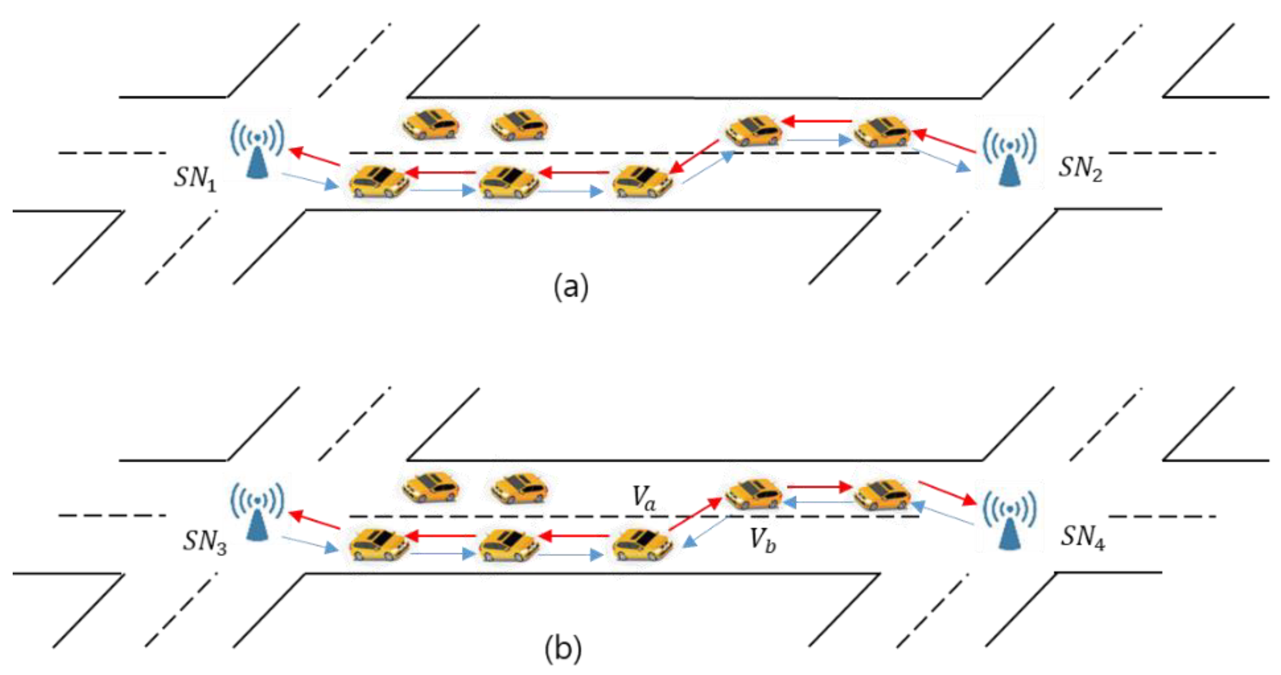
3.2.5. Two Conditions of Link Discover

If an SN finds that the link between it and the adjacent SN is broken (link expires), the node broadcasts a message (as shown in Table 2) to a vehicle on the corresponding road segment. In one condition, the vehicle selects the next-hop vehicle according to the above formulas until the message reaches the target intersection node. Then, the target intersection $S{N}_2$ sets up the reverse path from all vehicles back to the source intersection $S{N}_1$ (Figure 2a). In another condition, vehicles $V_a$ and $V_b$ find that each of their source intersection is the other’s target intersection (Figure 2b). Each vehicle then adds the other’s link information to its own table to form a complete link path between two adjacent intersection nodes, and update the new link information along the reverse path to two intersection nodes.

3.3. Intersection Decision

In this section, we will present routing over an SN (intersection node) level. Based on the information stored in the memory about the neighbor vehicle and the link connection information, we also employ other features for selecting the next best SN to forward data. The features include a 2-hop neighbor, the count of the vehicle in a whole link, the link lifetime, and the vehicle density on the segmented road between two SNs. The three features are described as follows:

• 2-hop neighbor: each SN keeps the information around itself in 2-hop. If a vehicle has a 2-hop neighbor, we consider the SN between them as the best candidate vehicle.
• The number of the vehicle in the effective link: the hop count recording starts whenever a link is created. Finally, the hop count of a link is recorded in the SN as a factor of an SN that can further choose the next hop.
• The link lifetime: longer link lifetimes are better for data forwarding. We assume that the link lifetime is the shortest lifetime between two vehicles which are in the same link as the standard. Each vehicle calculates and keeps the shortest lifetime and forwards it to the SN.

Before the selection of the SN, several steps are taken into account as shown in Figure 3.

DSN is the destination static node which is the two SNs located at both ends of the road segment where the destination vehicle is located.

• If the SN has only one 2-hop neighbor, the data packet is forwarded along with the link to the next SN.
• If the SN has more than one 2-hop neighbors, the SN selects the road segment with the highest degree of connectivity and the one which is geographically closest to the destination. The degree of connectivity is calculated based on the other two features using the following equation:

  $${\mathrm{Deg}}_{\mathrm{i}}={\mathrm{w}}_1{\mathrm{N}}_{\mathrm{i}}+{\mathrm{w}}_2{\mathrm{T}}_{\mathrm{i}},\mathrm{i}=1,2\dots \mathrm{n},$$

  (11)

  where ${\mathrm{N}}_{\mathrm{i}}$ is the number of vehicles in the effective link and ${\mathrm{T}}_{\mathrm{i}}$ is the link lifetime.
• If the SN has no 2-hop neighbor, but its neighbor SN is located on the destination segment which is also the destination vehicle, then the packet is forwarded to the neighbor SN. Otherwise, the packet is forwarded back to the last SN with more than one 2-hop neighbors and a suboptimum SN is chosen for forwarding the packet.
• When the packet arrives at the SN located at the destination segment and the packet cannot be forwarded to the destination immediately, the packet is forwarded toward another DSN.

The pseudocode of the intersection decision is described in Figure 4.

3.4. A Brief Description of the Routing

Figure 5 simply shows the working process of the proposed IRFMFD protocol. Source vehicle S sends packets to destination vehicle D. First, vehicle S selects a neighbor vehicle as the next hop which is a point in the link path between two adjacent intersections, and the packets are forwarded to an SN located at the intersection. Second, the SN chooses the next SN which keeps a link path between them, and the packets are forwarded to the next intersection until it reaches the destination vehicle.

4. Results

In this section, the simulation experiments are shown to evaluate the performance of the proposed routing protocol. To evaluate and compare the performance of IRFMFD, GPSR, GeOpps, and AODV, the simulations were performed with the same parameters.

4.1. Simulation Setting

IRFMFD was simulated using an NS2 simulator, with a mobility model consisting of an area of 3000 m × 4000 m. This was constructed using SUMO and formed a map shown in Figure 6a, which contained 28 junctions and 43 bidirectional road segments with four lanes. Figure 6b shows the view of an intersection. The initial positions and destination of vehicles are randomly distributed. The simulation parameters are shown in

Table 5. Simulation parameter.

Parameter	Value
Simulation area	3000 m × 4000 m
Number of vehicles	100, 150, 200, 250, 300, 350, 400
Vehicle speed	5–20 m/s
Radio range	250 m
Data packet size	1 k
Packet sending rate	4 pkt/s
Traffic Type	Constant bit rate (CBR)
Time to Live (TTL) of Packet	60 s
Simulation time	1000 s

. The vehicles moved with a speed ranging from 5–20 m/s. The transmission range was set to 250 m and the period of the traffic light was set to 50 s. The number of vehicles varied from 100 to 400, and the packet sending rate was set to 4 pkt/s. The simulation time duration was 1000 s.

4.2. Simulation Results

As shown in Figure 7, as the number of vehicles increases, so does the delivery ratio. This is because the higher network density provides a greater chance of successful transmission for forwarding packets to the destination. Simultaneously, the network density increases which also leads to a lower delivery delay as shown in Figure 8. Figure 9 shows changes in the number of hops of each routing protocol as the vehicle increases.

5. Discussion

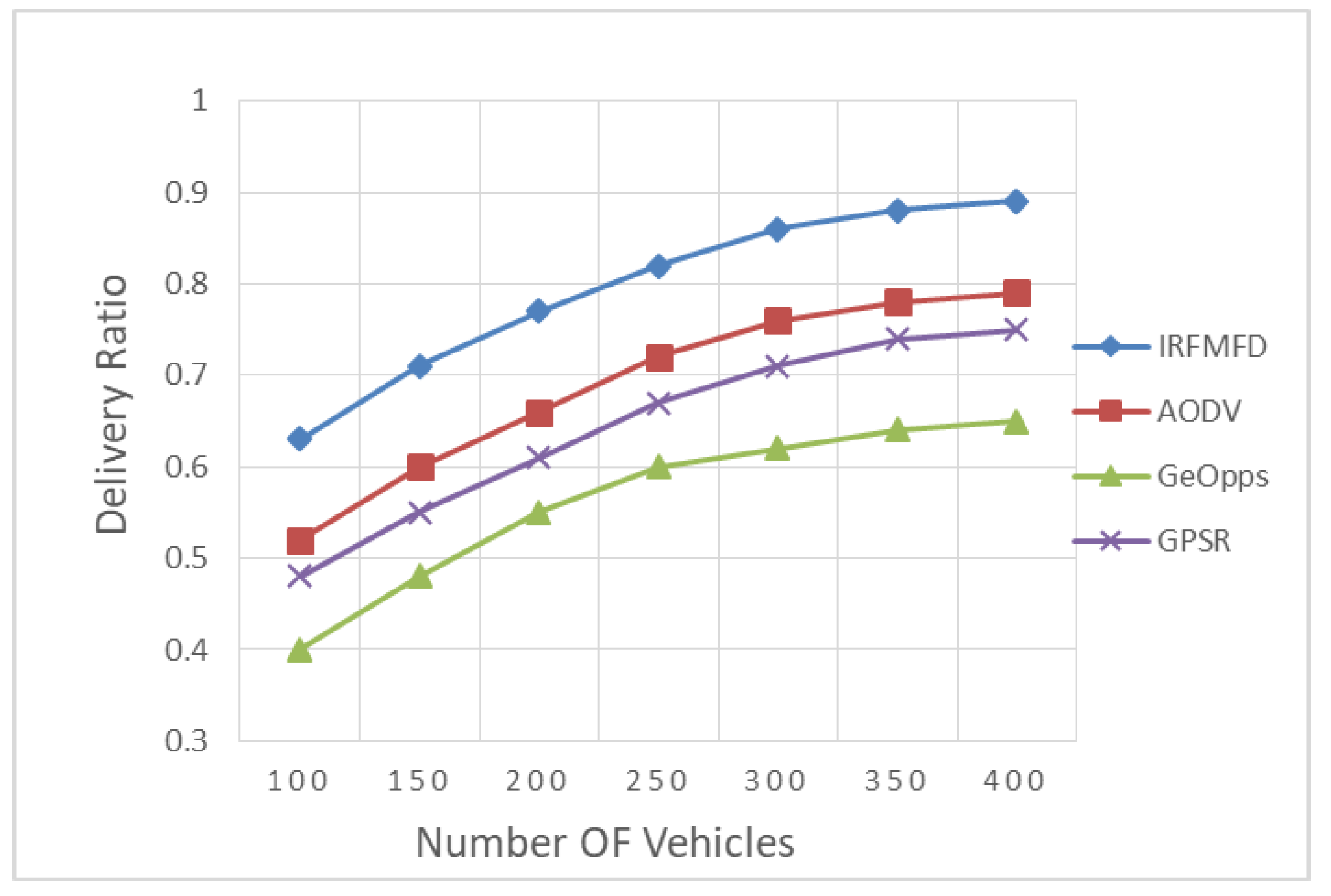
The performance of IRFMFD is better than AODV, GeOpps, and GPSR in the context of delivery ratio as shown in Figure 7 with an increasing number of vehicles. As mentioned before, the GeOpps is a DTN vehicular routing protocol, and it is designed to adapt to the environment in which packets are carried by the vehicles to the destination. Thus, this limitation of the GeOpps protocol makes it difficult to cope with the scenario where vehicles are carrying a high number of packets. The performance of GPSR is unsatisfactory because it only considers a single factor which is the geographic distance between the vehicle with the packet and the destination. The AODV outperforms GPSR and GeOpps in common urban environments where the speed of vehicles is not very fast and the topology does not change rapidly. Also, the AODV can adapt to changes more quickly than GeOpps and GPSR. The IRFMFD shows the best performance on delivery ratio because more elements are taken into account to decide for selecting the next-hop vehicle to forward the packet. Furthermore, it exhibits the characteristics of the topology-based routing protocols between two adjacent SNs.

Figure 8 also reveals that the IRFMFD, GPSR, and GeOpps show almost similar performance on the end-to-end delivery delay. However, the AODV has the highest delay compared with the others because the AODV establishes a route between packet carrier and destination to forward the packet. This strategy makes it possible for the packet-carrying vehicles to keep the packet for a long time in order to increase the delivery delay. However, since the path to SN has been established in advance, the packet-carrying vehicles do not need to wait.

As shown in Figure 9, IRFMFD has more hop count compared with other routing protocols. This is because the choice of each hop of IRFMFD has more constraints. It also inevitably increases some unnecessary hop that the packets have to be forwarded to every SN. At the same time, more hop count also increases the data delivery ratios.

In the future, our work will be focused on the routing design supported by 5G and blockchain technology. We will study and analyze which characteristics of vehicles are more suitable for 5G and blockchain technology. It is foreseeable that vehicles will be equipped with a large number of sensors in the future and that data collection and sharing will be greatly supported by 5G and blockchain technology.

6. Conclusions

In this paper, IRFMFD improves routing performance in VANETs for urban environments, which is achieved through vehicle decision and intersection decision. Vehicle decision calculates a fuzzy performance score to choose the next-hop vehicle between SNs located in the intersections using three factors. Intersection decision preferentially selects SNs with 2-hop neighbors, with the introduction of three factors if there is more than one candidate. By using the fuzzy number and introducing multiple factors simulation results show that the IRFMFD performs better with a high delivery ratio and low end-to-end delay than other protocols used for the same purpose in the literature.