Scheduling in Heterogeneous Distributed Computing Systems Based on Internal Structure of Parallel Tasks Graphs with Meta-Heuristics

Abstract

The problem of scheduling parallel tasks graphs (PTGs) represented by directed acyclic graphs (DAGs) in heterogeneous distributed computing systems (HDCSs) is considered an nondeterministic polynomial time (NP) problem due to the diversity of characteristics and parameters, generally opposed, intended to be optimized. The PTGs are scheduled by a scheduler that determines the best location for the sub-tasks that constitute the PTGs and is responsible for allocating the resources of the HDCS to the sub-tasks of the PTGs. To optimize scheduling and allocations, the scheduler extracts characteristics from the internal structure of the PTGs. The prevailing characteristic in existing research is the critical path (CP), which is limited to providing execution paths of PTGs; considering this limitation, we extend the array method proposed in Velarde, which extracts two additional characteristics to the CP: the layering and the density of the graph for scheduling. These characteristics are represented as integer values of the PTGs to be scheduled; the values obtained from the characteristics are stored in arrays representing populations that are evaluated with the heuristic univariate marginal distribution algorithm (UMDA) and in terms of comparison with the genetic algorithm. With the best allocations produced by the algorithms, two performance parameters are evaluated: makespan and waiting time. The results indicate that when more PTGs characteristics are considered, resource allocations are optimized, and scheduling times are reduced. The results obtained with the heuristic algorithms show that UMDA provides shorter scheduling and allocation times compared with the genetic algorithm; UMDA widely distributes the sub-tasks in the clusters, whereas the genetic algorithm compacts the assignments of the PTGs in the clusters with a longer convergence time that translates into longer scheduling and allocation times. Extensive explanations of these conclusions are provided in this work, based on the conducted experiments.

1. Introduction

The diversity of the characteristics of heterogeneous distributed computing systems (HDCSs), such as the speed of the processors, the number of cores per processor, the geographic distances between processors, and the number of local networks, among others, make it difficult to optimize resource use when seeking to maximize computing power with parallel applications. One of the most widespread methods used to program parallel applications running on HDCSs is through parallel tasks graphs (PTGs) [1]. The PTGs are constituted by a set of sub-tasks that are assigned in the HDCS computer resources for their execution [2,3] through a previous scheduling. The scheduling and allocation are performed by a scheduler that works in two phases: first, it schedules the sub-tasks using the characteristics of the PTGs and the HDCS resources, and second, it allocates the sub-tasks of the PTGs to the target resources, where each sub-task is executed until its completion [4,5,6,7,8]. The following two paragraphs describe each phase of a PTG scheduler in an HDCS, to explain the general context of this research and thus facilitate its understanding.

The task scheduling phase requires an analysis of the characteristics of the PTGs. The most frequently used characteristic is the Critical Path (CP), which defines the structure of a graph and is obtained by traversing all the paths from the start node to the end node of the PTG. By definition, this is the most expensive path in the execution of a PTG [5,6,7,9,10], and it is high priority in the allocation of resources to speed up the execution of the application. Other characteristics also define the graph’s internal structure, such as the graph density and layering [11,12]. The graph density allows seeing how much information is transferred between sub-tasks in the PTGs, whereas the layering determines the number of sub-tasks per PTG level. These two features, in addition to the CP, when considered in the scheduling of the PTGs, can speed up scheduling and optimize the resource allocations of the HDCS, as shown in this paper. The task allocation phase requires placing each sub-task of the PTG to a HDCS resource, where it remains until the completion of its execution. To optimize the execution of the PTGs, the allocation considerations in this work include two determining factors:

• the proximity of the sub-tasks that have dense communication, which can be obtained by means of graph density, and
• the permanence of the sub-tasks of a PTG in the same cluster, considering the layering as a determining factor for the assignment.

To conduct experiments with both factors, PTGs should be created randomly with sufficiently heterogeneous characteristics and the schedulers should be evaluated in uncontrolled environments [13]. In addition, it is necessary to consider the generation of PTGs from real applications.

This paper extends the array method [8], a scheduler whose functionality is based on the extraction of three characteristics: CP, graph density, and layering of the PTGs that remain in a queue for execution in an HDCS (in this paper, the terms HDCS and target system are used equivalently). The characteristics of each PTG are represented as integer values that are stored in arrays that are used to generate allocations in the target system and, with these allocations, produce populations that are later evaluated by two algorithms: Univariate Marginal Distribution Algorithm (UMDA) and genetic algorithm. Evaluations with both algorithms produce the best allocations of sub-tasks to HDCS resources, with the aim of optimizing two performance parameters, which are graphed to observe and describe their results.

The performance parameters that are evaluated in this paper are makespan and waiting time. The makespan evaluates the total execution time of the parallel task [6], and the waiting time is the time a PTG waits for its scheduling and allocation in the HDCS. The results obtained from the evaluations show that the UMDA exceeds the genetic algorithm in the scheduling speed and resource allocation but significantly lacks a process for task grouping in the clusters, causing a disaggregation of sub-tasks that belong to a PTG. The genetic algorithm has slower scheduling and allocation times but it achieves closer sub-task groupings of PTGs, which optimizes communication times between tasks.

This research, which extends a previously published method [8], includes six new contributions, as described below.

First, in [8], only one algorithm for random task generation was used, and thus, we used the following.

• The Markov chain algorithm [14] for the random generation of PTGs, whose main feature is the generation of PTGs with a greater distribution of sub-tasks in the initial phase, allowing a rapid consumption of resources and observing the behavior of the heuristic algorithms.
• The parallel approach for the random generation of graphs on Graphics Processing Units (GPUs) [15], shows a thinning of the width of the PTG, and each level produces a substantial number of edges, indicating the parallel applications with high rates of communication between them, allowing evaluation of the communication times of the target system [13].

Second, two performance parameters—makespan and waiting time—are evaluated separately with each of the above algorithms to evaluate the proposed scheduler in terms of its response times with different workloads as follows,

• the makespan parameter, which is the most widely used parameter in the literature to evaluate a schedulers’ performance, which provides a perspective on the total time each of the PTGs remains in the HDCS from their arrival in the queue to the end of their execution, and
• the waiting time, which is the time that a PTG waits for scheduling and allocation in the queue of the HDCS. This parameter provides an evaluation of the scheduler’s response times.

Third, the number of clusters in the target system is increased to evaluate the growth of the resource matrix, and the response times of the algorithm when many processors remain available.

Fourth, an example is provided of the array method to show how it works and to achieve an understanding of its concepts and algorithms.

Fifth, the quality parameter of the allocations is evaluated to verify the percentage of allocated (used) resources of the HDCS once each of the algorithms (UMDA and genetic) performs the scheduling and allocation. Evaluating the quality of allocations is important because it measures the performance of the algorithm when increasing and decreasing the number of resources available in the HDCS; it also allows observing the behavior of each of the algorithms with a minimum or maximum amount of resources, which represents the optimization of resources.

Sixth, the section on basic definitions is extended for a broader understanding of the proposed scheduler.

The remainder of this paper is structured as follows. Section 2 presents a set of terms and the UMDA (the base algorithm used in this paper). Section 3 summarizes related studies that deal with scheduling problems and critical paths, and studies that proposed solutions to the layering problem in Directed Acyclic Graph (DAG) tasks. Section 4 explains the array method with an example using the basic concepts in Section 2; then, Section 5 describes the experiments and the results obtained on the hardware and software platforms. Section 6 provides a discussion of this work. Section 7 outlines the subsequent studies that are currently being carried out, and Section 8 describes the materials and methods used to carry out this research. Finally, Section 7 presents the conclusions of this work.

2. Basic Definitions

This section defines a set of terms to help understand the following sections in this paper. It considers the definitions contained in [8,13] and other definitions arising from the extension of this research. An additional subsection to explain the UMDA is provided.

Definition 1.

The target system is constituted by $C_k$ clusters $C_1,C_2,...C_k$, where k is the number of clusters of the HDCS. Each cluster contains m heterogeneous processors with n processing cores. Therefore, $C_{k,n,m}$ denotes the core k processor n processing core m.

Definition 2.

A PTG can be modeled by a directed acyclic graph (DAG) $T=(N,E)$, where $N=\{{\eta }_i:i=1,...,N\}$ is a set of N nodes or sub-tasks and $E=\{E_{i,j}:i,j=1,...,N\}$ is a set of E edges. Parallel task graph T can be characterized by $({\eta }_i,\{1\le j\le {\eta }_i|{\tau }_{i,j}\},G_i,V_i,W_i)$, where ${\eta }_i$ is the number of sub-tasks of $T_i$, the second parameter is the set of sub-tasks, $G_i$ is the set of relations directed between the sub-tasks, $V_i$ is the number of levels of ${\tau }_i$, and $W_i$ the width of each level of ${\tau }_i$ (represented by a vector). The PTG consists of a set of nodes and edges (directed relationships). The nodes represent the execution requirements of the task, whereas the directed relationships show the execution flow.

Definition 3.

A directed relationship from sub-task ${\tau }_{i,j}$ to ${\tau }_{i,k}$ means that ${\tau }_{i,k}$ can start its execution only if ${\tau }_{i,j}$ completes its own. In this case, we call ${\tau }_{i,j}$ a parent sub-task of ${\tau }_{i,k}$ and ${\tau }_{i,k}$ the child of ${\tau }_{i,j}$. Each sub-task in a given DAG task can have several parents and children. An initial sub-task is a sub-task without parents, whereas a final sub-task is a sub-task without children. A PTG has a start sub-task and a finish sub-task.

Definition 4.

Layering. Given T, where each $n\in N$ node has a positive width $W_i$, a division by layers or levels of $T_i$ (also called stratification of $T_i$) is a partition of its set of nodes V within disjointed subsets $V1,V2,...,Vh$, such that if $(u,v)\in E$, where $u\in V_i$ and $v\in V_j$, then $i>j$. A DAG with a stratification or division by levels is called a stratified digraph.

Definition 5.

The width of a level $V_k$ is traditionally defined as $w\left(V\right)={\sum }_{v\in V_k}$, and the width of a stratified digraph (divided into layers or levels) is defined by the equation $w=ma{x}_{1\le k\le h}w\left(V_k\right)$

Definition 6.

The height of a vertex is denoted by [6]:

$$height\left(n_i\right)=\left\{\begin{array}{c}0ifPRED\left(n_i\right)=Ø\hfill \\ \\ 1+max\left(height\left(n_j\right)\right)\forall n_j\in PRED\left(n_i\right)otherwise\hfill \end{array}\right.$$

(1)

Definition 7.

The set of DAG tasks that represents a synthetic load is denoted by $\tau =\{{\tau }_1,...,{\tau }_n\}$.

Definition 8.

The length of the critical path of a DAG task [6], is denoted by

$$M=\lceil \frac{\sum W_{n_i}}{cplength}\rceil$$

where M is the minimum number of processors and $W_{n_i}$ is the processing time of task i.

Definition 9.

The cost of calculating an execution cost (EC) of a sub-task represented by a node expressed in flops is the cost of executing a sub-task once it is assigned to a processor. The cost of executing the total of the sub-tasks of task i is expressed as

$$\sum _{\forall {\tau }_{i,j}\in {\tau }_i}^{}E{C}_{i,j}.$$

(2)

Definition 10.

The cost of communication represented by $C{C}_{{\tau }_{i,j}\to {\tau }_{i,k}}$ between sub-tasks ${\tau }_{i,j}$ and ${\tau }_{i,k}$ is expressed in bytes.

Definition 11.

Makespan, the length of the scheduling produced by the algorithm, is expressed as

$$makespan=max\left(FT\left(n_i\right)\right).$$

(3)

Definition 12.

The start time of the task is the start time of each DAG task and is calculated according to:

$$S_t\left(T_n\right)=E{X}_t\left(\sum _{T_1}^{n-1}\right)+DC{T}_t\left(\sum _{T_1}^{n-1}\right)+S{T}_{T_n\to {\pi }_m},$$

(4)

where $S_t\left(T_n\right)$ is the start time of the task, $E{X}_t\left({\sum }_{T_1}^{n-1}\right)$ is the execution time of its predecessor nodes, $DC{T}_t\left({\sum }_{T_1}^{n-1}\right)$ corresponds to the data communication time of its predecessor nodes, and $S{T}_{T_n\to {\pi }_m}$ is the sending time of the task to the processor.

Definition 13.

The task completion time (TCT) is the time that is recorded in the matrix once the task has finished its execution in the processor; the parameter is calculated by

$$TCT=S_t\left(T_n\right)+TaskExecutionTime.$$

(5)

Definition 14.

The quality of the allocations represents the percentage of occupied processors in each allocation made by the algorithms, and is calculated as the total sum of processors that are occupied in the allocation, among the total number of processors in the target system times 100. The quality of the allocations is obtained with

$$Q_a=\left(\frac{{\sum }_{i=0}^m\forall {\pi }_{m}thatcontainsa{\eta }_i}{\left|\pi \right|}\right)\times 100.$$

(6)

With the aforementioned definitions, we consider an HDCS with $C_k$ clusters and synthetic load $\tau$ of tasks. Each PTG is scheduled in the $C_k$ cluster set by means of a scheduler respecting the execution requirements, the directed relationships, and the start times of each DAG task.

UMDA

Distribution Estimation Algorithms (DEAs), are evolutionary algorithms that use a collection of candidate solutions to perform search paths avoiding local minima [16,17]. These algorithms use the estimation and simulation of the joint probability distribution as an evolutionary mechanism instead of directly manipulating the individuals that represent solutions to the problem. In a DEA, a population of individuals represents solutions to the problem. Three types of operations are iteratively performed on the population: generating a subset of the best individuals in the population, learning a probability distribution model from the selected individuals, and new individuals are generated by simulating the obtained distribution model. The algorithm stops when a certain number of generations is reached or when the population’s performance stops significantly improving.

To estimate the joint probability distribution at each generation from the selected individuals, the univariate marginal distribution algorithm (UMDA) is used. Thus, the joint probability distribution is factored as the product of independent univariate distributions [16,18], i.e.,

$$p_l\left(x\right)=p(x\mid D_{l-1}^{Se})=\prod _{i=1}^n{p}_l\left(x_i\right).$$

(7)

Each univariate probability distribution is estimated from the marginal frequencies:

$$p_l\left(x_i\right)=\frac{{\sum }_{j=1}^n{\delta }_j(X_i=x_i\mid D_{l-1}^{Se})}{N}$$

(8)

where

$${\delta }_j(X_i=x_i\mid D_{l-1}^{Se})=\left\{\begin{array}{c}0ifinj-th{D}_{l-1}^{Se},X_i=x_i\\ 1inothercase\end{array}.\right.$$

(9)

The definitions in this section are explicitly referenced in the following sections.

3. Related Works

This section describes research work in which contributions in the area of scheduling using the structure of the PTGs are highlighted.

3.1. Scheduling Problems and Critical Paths

Qamhieh et al. [2] analyzed the DAG tasks considering the internal structure and execution flow of the DAGs. They presented the optimal scheduling algorithm global earliest deadline first (global EDF) for scheduling in homogeneous multiprocessor systems; it is a fixed work priority allocation algorithm in which the DAG task with the first absolute deadline has the highest priority. Mustafizur et al. [10] described the dynamic critical path for grids (DCP-G) algorithm that makes use of two execution parameters: absolute execution time (AET), defined as a minimum execution time according to the size of the task, and absolute data transfer time (ADTT), which is defined as the minimum time required to transfer the task output given its current location on the grid. Ahmad et al. [6] proposed a solution based on the evolutionary stochastic technique known as particle swarm optimization (PSO) in three consecutive steps using the critical path of the PTGs: preparation of the graph, representation of the solution, and particle generation. The scheduling is evaluated after assigning each task to its corresponding processor by calculating the capacity of the particles. The best particle is the one with the minimum makespan. Takpe et al. [5] presented a solution based on a heterogeneous collection of homogeneous C clusters with identical processors. The main objective is to assign parallel tasks within a single cluster using a critical path algorithm. The algorithm proceeds in two steps: allocation and placement. In the first, the reference allocation is determined and a function is designed to deduce the number of processors to be assigned to a task in each cluster. In the second step, each completed task is allocated according to the earliest possible completion time. Minhaj et al. [7] started from the intuitive assumption that effective scheduling occurs when the tasks on the critical path are scheduled first. The scheduling proceeds is as follows. First, the graph is walked initially, and critical paths are found based on two costs: average costs of execution and the communication costs of the sub-tasks. Second, the processors are allocated, using queues based on restricted critical path and containing tasks ready for scheduling. Duk et al. [9] presented the Critical Path Identification (CPI) method, which analyzes the characteristics of workflow control structures. It is based on the average execution time of the activities and it systematically determines the critical path in a workflow.

3.2. Solutions to the Layering Problem in DAG Tasks

To stratify DAG tasks, layers are applied and sets of vertices are divided into subsets so that the nodes connected by a directed route belong to different subsets. The subsets are assigned whole ranges so that the range of the subset that contains the edge is smaller than the range of the subset that contains its ancestor edge [11]. In current studies, different methods have been proposed to stratify a graph [11]. Three widely used stratification algorithms find the disposition of a DAG task; they are subject to some of the following aesthetic criteria: the longest path algorithm, the Coffman–Graham algorithm, and the Gansner ILP (Integer Linear Programming) algorithm [12]. In graph stratification studies, two aesthetics of the graph are sought: stratification area and the number of fictitious nodes that introduce the algorithms [12]. For node stratification, we did not consider the aesthetics of the graph in this study.

4. Array Method

This section defines the concepts and algorithms of the array method proposed in [8]. The operation of the array method is further explained and complemented using an example.

The array method neither modifies the PTG nor are subgraphs created during the analysis of the PTGs. The queue discipline that stores PTGs on arrival at HDCS is first come first serve (FCFS) and is large enough to accommodate PTGs.

The array method is a scheduler that uses procedures for filling a set of arrays in each of its two phases. The scheduling phase considers the procedures for filling the following arrays; resources, characteristics, allocations, and populations. The allocation phase considers the arrays of the start times of the tasks.

The following paragraphs describe each array and explain the procedures that generate the values for the arrays and how the arrays are used to build the populations that are evaluated by the UMDA and genetic algorithm.

4.1. Task Scheduling Phase

4.1.1. The Resource Matrix

Definition 15.

The Resource Matrix, is a symmetrical matrix that stores the characteristics of the resources.

Consider an HDCS, as shown in Figure 1, similar to the system previously proposed [19]. In our case, the system is constituted by three clusters joined by a high-speed network; each cluster is formed by different commodity processors and different number of processing cores in each commodity processor.

The cluster is characterized in the

Table 1. Resource matrix. Symmetric matrix with distance between HDCS processors from Figure 1.

	1	2	3	4	5	6	7
$C_1$$1_2$	0	1	1	1	1	1	1
$C_2$$2_2$	1	0	0	0	1	1	1
$C_2$$3_4$	1	0	0	0	1	1	1
$C_2$$4_8$	1	0	0	0	1	1	1
$C_3$$5_2$	1	1	1	1	0	0	0
$C_3$$6_4$	1	1	1	1	0	0	0
$C_3$$7_4$	1	1	1	1	0	0	0

resource matrix according to Definition 1. For our sample case, Table 1 shows the resource matrix of the HDCS in Figure 1 using three clusters. Then, using Definition 1, $C_{k,m,n}$ represents cluster k, processor m, and processing core n. Thus, $C_{1,1,2}$ represents cluster 1, processor 1, and processing cores 2. The positions of the matrix that contain 0 represent the processors that remain in the same network. Although the distance of the processors is 0, the communication time must be considered at the start time of all the tasks. A list of the main steps of the algorithm to create resource matrix is provided in Algorithm A1.

The columns that constitute the resource matrix include the following.

• Resource ID number: an incremental number generated according to its integration to HDCS.
• Number of processing cores of the resource: identified by an integer that represents the number of processing cores of each processor according to Definition 1.
• Distance from one resource to another: a value obtained from the distance (the number of jumps) from one processor to each of the processors in external clusters.

When a new resource is added to the HDCS, its features are extracted and placed into this matrix using the feature extraction and resource sorting algorithm (the algorithm for verification of new resources in the system is provided in Algorithm A1).

The resource matrix aims to solve the problem of changes in resource availability [10], which occurs during the release and allocation of resources.

The procedure for filling and updating values in this matrix is performed with the algorithm for verification of new resources in the system, as shown in Appendix A. Processor speeds were not considered in this study.

4.1.2. The Characteristics Matrix of the Evaluated DAGs

Definition 16.

The Characteristics Matrix of the evaluated DAGs is a data structure that stores the data obtained by the feature extraction algorithm.

This array is composed of the following columns.

• DAG ID number, which is allocated according to arrival to the queue of the system.
• The number of paths of the DAG, which are extracted by means of the depth first search (DFS) algorithm, with a worst-case temporal complexity of $O\left(b^m\right)$. By means of DFS, all the execution paths of the PTG are extracted with their lengths, obtaining the execution and communication from each path.
• The number of levels of the DAG and the number of vertices per level: a stratification or division by levels; see Definition 4 in Section 2.
• DAG density: The density of the graph denotes the number of edges between two levels of the DAG. With a low value in this property, there are few edges; with large values, there are many edges in the DAG.

The procedure for filling the characteristics matrix is as follows. Once DFS is run in the system, the PTG execution paths are found, the costs of each task are sorted to obtain the PTG critical path (the path that generates the highest execution costs as calculated using Definition 8) with the highest scheduling and allocation priority. The remaining paths are considered as sub-critical paths and have a decreasing priority in the allocation of system resources. The number of PTG levels (Definition 4) and the number of vertices of each level are also generated during the same execution of the DFS algorithm.

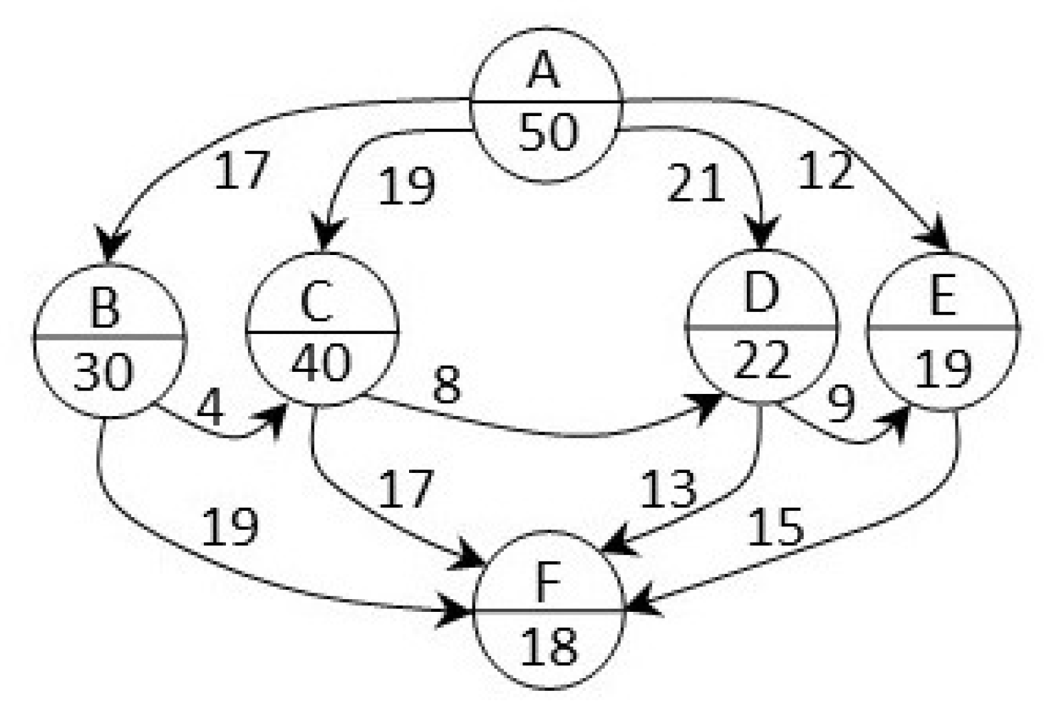
The matrix of characteristics in this example considers the PTGs in Figure 2 and Figure 3 that contain the same number of nodes. For this example, Figure 2 represents PTG ID 1 and Figure 3 represents DAG task ID 2. The characteristics of both PTGs are placed in

Table 2. Characteristics matrix of the Parallel Task Graphs (PTGs) from Figure 2 and Figure 3.

DAG ID	DAG Paths	Path Nodes	Number Level	Nodes Per Level	DAG Density
1	1	ABDF	1	2	0-1 → 2
1	2	ABEF	2	2	1-2 → 3
1	3	ACF			2-3 → 2
2	1	ABF	1	4	0-1 → 4
2	2	ABCF			1-2 → 4
2	3	ABCDF
2	4	ABCDEF
2	5	ACF
2	6	ACDF
2	7	ACDEF
2	8	ADF
2	9	ADEF
2	10	AEF

to represent the matrix of characteristics of both PTGs. This table contains all the information of the analyzed PTGs.

4.1.3. The Allocation Matrix

Definition 17.

The allocation matrix is a dynamic matrix that grows or decreases as the search for resources for the PTGs is carried out.

This array is composed of the following columns.

• System processors with their number of cores, according to Definition 1 in Section 2.
• PTG sub-task identifier according to Definition 2 in Section 2.

The procedure for filling the allocation matrix is as follows. With the characteristics matrix of the PTGs, it is possible to start the process of searching for the resources in the HDCS, which performs the filling of the characteristics matrix.

The sub-task to a resource is allocated based on the characteristics of the PTGs, which, in the execution of the algorithm, are called search criteria. The following paragraphs describe in detail how the algorithm proceeds to search the resources in the HDCS.

The first search criterion is the PTG paths. The resource allocation process is started using each of the routes in the DAG considering the first path in the characteristics matrix (column 2 DAG paths, Table 2) as the critical path with the highest allocation priority; the rest of the paths are considered subcritical paths by the algorithm. The vertices of the PTG that constitute the critical path are trimmed, and then each of the subcritical paths is trimmed. The algorithm checks the processing cores in each processor with the number of nodes in each path. Depending on the number of nodes in the path, it looks for a processor with a number equal to or less than the number of nodes in the path. If the number of nodes in the path is greater than the maximum number of cores than one (or more) of the system processors, then it applies the divide and conquer method: it divides the number of nodes in the path by two, rounds down to the lowest number, and then looks again for a processor with the number of nodes obtained with the division. If, with this division, it is not possible to cover the number of nodes in the path again, the two results are again divided by two. This condition ends when it obtains a number of nodes that can be covered by the number of processor cores in the system.

When a PTG sub-task is likely to be allocated to the resource in the row, the column is marked with a value of 1, indicating the processor as a candidate to contain the sub-task. The algorithm seeks to allocate one sub-task per processing core, which avoids overloading threads or processes in each core.

The allocation matrix is updated if a processor is located for the sub-task; the update occurs with the PTG sub-tasks and the cores of each processor as follows. If a processor meets the condition of the number of cores equal to or less than the number of nodes in the path, then this processor is placed in the allocation matrix, indicating which DAG nodes will be allocated to that processor. This allocation of cores to nodes indicates how many nodes of the DAG will remain in the same cluster for processing and how many nodes of the DAG must be placed in other clusters. With the diversity of clusters where the nodes are allocated, the distance is calculated to determine the communication load. Definition 10 (overhead) is used to generate the task during its processing. It is clear that the minimization function will seek to process all the nodes of the DAG in the same cluster.

For the example described in this paper,

Table 3. Example of a first assignment in the grid for the Figure 2 DAG task using the DAG task paths (each solution is shown in a different shade of gray).

	A	B	C	D	E	F	HD
$C_1$$1_2$	0	0	0	0	0	0
$C_2$$2_2$	0	0	1	0	0	0
$C_2$$3_4$	1	1	0	1	0	1
$C_2$$4_8$	0	0	0	0	1	0	0
$C_3$$5_2$	0	0	1	0	0	0
$C_3$$6_4$	0	0	0	0	1	0
$C_3$$7_4$	1	1	0	1	0	1	0

and

Table 4. Example of a second assignment in the grid for the Figure 2 DAG task using the DAG task paths (each solution is shown in a different shade of gray).

	A	B	C	D	E	F	HD
$C_1$$1_2$	0	0	1	0	0	0
$C_2$$2_2$	0	0	0	0	1	0
$C_2$$3_4$	0	0	0	0	1	0
$C_2$$4_8$	1	1	0	1	0	1	1
$C_3$$5_2$	0	0	0	0	0	0
$C_3$$6_4$	1	1	0	1	0	1
$C_3$$7_4$	0	0	0	0	0	0	2

show the allocation of the graph in Figure 2 using the DAG paths (each solution is shown in a different shade of gray). The PTG has four vertices. The algorithm looks for a first allocation of a processing element (PE) of four cores. If it is not able to locate the path in a PE with this number of cores, it will seek to assign two dual core PEs with a minimum distance, considering that the minimum value of the distance is 0, which corresponds to a processing element within the same local network (LAN). The next step is to look for the allocation of the next path of the DAG without considering the vertices already allocated; for the example in question, vertex D is allocated and a subsequent step aims to allocate vertex E, both with a dual core PE. If a PE with these characteristics is not obtained, it will look for two PEs.

The second search criterion for the allocation of resources is the levels of the PTG. The information provided by the PTG levels is the number of PTG levels and the number of vertices per level (see Definition 4). For the case of the PTG in Figure 2, allocating by paths is the most feasible process to accelerate the execution of the task, but this is not the case for the PTG in Figure 3 due to the large number of paths generated. For this case, the algorithm seeks to assign only three PEs as follows. For the case of level 1, it looks for a PE with a processing core; for level 2, the algorithm looks for assigning a PE with eight processing cores (according to Definition 3); and for the last level of the DAG, it looks for a PE of a single core, or in its case, a dual core.

For all three PEs, it is necessary to look for the minimum distance. Once the three PEs are assigned, the DAG is processed sequentially so that the processing data flows in one direction. If the algorithm does not locate an octa-core PE, the divide and conquer method is applied again. The aim is to locate two quad-core PEs with a minimum distance. With this second search criterion, the assignment matrix is created to allocate the nodes to the processing cores of each processor, exactly as the allocation was made for the DAG paths.

For the case of the PTG in Figure 3, given space limitations, only one solution is shown in

Table 5. Example of a first assignment in the grid for the Figure 3 DAG task using the DAG task paths.

	A	B	C	D	E	F	HD
$C_1$$1_2$	1	0	0	0	0	0
$C_2$$2_2$	0	0	0	0	0	1
$C_2$$3_4$	0	1	1	1	1	0	1
$C_2$$4_8$	1	1	1	1	1	1	0
$C_3$$5_2$	0	0	0	0	0	0
$C_3$$6_4$	1	1	1	0	0	0
$C_3$$7_4$	0	0	0	1	1	1	0

. For this case, three solutions (each solution is shown in a different shade of gray) are presented, each with its respective calculation of processor distances in the HDCS.

In conclusion, for the allocation matrix of this example, due to space reduction, only the processors selected in the allocation process are listed. Table 3, Table 4 and Table 5 represent allocation solutions to the HDCS of the PTG in Figure 2 and Figure 3 using the run paths. In this case, possible assignments or solutions are generated (each assignment is shown in different colors of gray). For each allocation produced, the distance D (last column of the array) is calculated. This value is used in

Table 6. Initial population. A first set of evaluation results for each parameter.

	${\mathit{S}}_1$	${\mathit{S}}_2$	${\mathit{S}}_3$	${\mathit{S}}_4$	${\mathit{S}}_5$	${\mathit{S}}_6$	${\mathit{S}}_7$	${\mathit{S}}_8$
Distance	0	0	1	2	1	0	0	1
Processor status	0	1	1	1	0	0	2	2
Distance to objective cluster	0	0	1	0	1	0	0	1
$h\left(x\right)$	0	1	3	3	2	0	2	4
$\widehat{p}$	0	0.75	0.33	0.33	0.5	0	0.5	0.25

and

Table 7. Initial population. A second set of evaluation results for each parameter.

	${\mathit{S}}_1$	${\mathit{S}}_2$	${\mathit{S}}_3$	${\mathit{S}}_4$	${\mathit{S}}_5$	${\mathit{S}}_6$	${\mathit{S}}_7$	${\mathit{S}}_8$
Distance	0	0	1	2	1	0	0	1
Processor status	0	0	1	1	0	0	0	2
Distance to objective cluster	0	0	1	0	1	0	0	1
$h\left(x\right)$	0	0	3	3	2	0	0	4
$\widehat{p}$	0	0	0.33	0.33	0.5	0	0	0.25

, called the initial population, in which each column $S_n$ represents a generated solution, with the respective values of each parameter.

4.1.4. Generation of the Population Matrix

First, the initial population is created from all the generated allocations (solutions) in the HDCS using the search criteria. For our example, some of the allocations in Table 3, Table 4 and Table 5 are shown in Table 6 and Table 7, which represent the initial population denoted by $P_0$, where $h\left(x\right)$ represents the sum of the independent variables and $\widehat{p}$ represents univariate probability distribution.

Second, some individuals are selected from $P_0$ through the standard truncation selection method. Half of the initial population is selected, denoted by $P_0^{Se}$. The selection is carried out by a function that minimizes the values of the three parameters. In the case of ties, when evaluating individuals, the selection is conducted using probabilistic means.

The joint probability distribution expresses the characteristics of the selected individuals. They are not considered to be interdependencies between variables, so they are considered to be independent from the rest; thus,

$P_1\left(x\right)=P_1(x_1,...,x_3)={\prod }_{i=1}^{3}p(x_i\mid D_0^{Se})$.

The model is specified with three parameters. For each parameter,

$p(x_i\mid D_0^{Se})withi=1,2,3$.

The parameter values are shown in the last rows of Table 6 and Table 7.

Table 8. File of cases for the solutions generated for the DAGs in Figure 2 and Figure 3; where $S_n$ represents a generated solution

${\mathit{S}}_1$	${\mathit{S}}_2$	${\mathit{S}}_3$	${\mathit{S}}_4$	${\mathit{S}}_5$	${\mathit{S}}_6$	${\mathit{S}}_7$	${\mathit{S}}_8$
$S_1$: 0	$S_2:0.75$	$S_3:0.33$	$S_4:0.33$	$S_5:0.5$	$S_6:0$	$S_7:0.5$	$S_8:0.25$
$S_1$: 0	$S_2:0$	$S_3:0.33$	$S_4:0.33$	$S_5:0.5$	$S_6:0$	$S_7:0$	$S_8:0.25$

represents the case consisting of the individuals obtained from the simulation of $P_1\left(x\right)$ extracted from Table 6 and Table 7.

The previous steps are repeated until the stop conditions are met, which is the maximum number of populations indicated in the algorithm, or when the population does not improve with respect to the best of the individuals obtained in previous generations.

4.2. Allocation of Processors to Tasks

In the phase of allocating processors to tasks, if the processor is free at the time of allocation, only the time of sending the task to the processor is considered. For the other case, if the processor is busy, the time that the task waits to be sent to the processor is considered.

In our case, an unoccupied processor has a higher probability of being allocated, whereas an occupied processor has a lower probability of being allocated. The task start time is calculated when all predecessor nodes have finished their execution.

4.2.1. Best Allocation Search

The UMDA is executed based on the results presented by the allocation matrix. The contents of the allocation matrix include the following.

• The distance of the nodes located on the processors. A high value in the indicates that the task was disaggregated into several clusters.
• The processor status parameter: occupied or unoccupied. An unoccupied processor is assigned a value of 0; an occupied processor is assigned a value of 1.
• The task location in the cluster parameter is a value obtained from the distance of the cluster where the queue of tasks from the cluster where the task can be executed. The value of this parameter depends on the number of clusters that the task must pass through to get to the cluster where it will be executed. For example, suppose that the task from DAG 1 is located in cluster 2 and cluster 3, then the task location parameter will take the value of the necessary time to locate the task in both clusters. When a task is located in the same cluster where the queue resides, this parameter takes a value of 0.

For our example case, the queue resides in cluster 1 and the results of the three parameters are shown in the allocation matrix (Table 3 and Table 4).

The different node allocations aim to minimize the distance that provides the location of the task in the cluster or in the clusters of the HDCS.

4.2.2. Matrix of the Start Times of the Tasks

Definition 18.

Matrix of the Start Times of the Tasks, stores the results of the calculations of the start times of each sub-task of the PTGs.

This matrix is constituted by the following columns.

• Task ID
• Task arrival time: The time at which the task was queued in the waiting queue.
• Task start time: This parameter is calculated according to Definition 12.
• Rask completion time: This time is calculated using the formula in Definition 13 and is recorded in the matrix when the execution on the processor is complete.

The procedure for filling the the matrix of the start times of the task, four parameters are used:

• Processor status. When the processor is unoccupied, the task can start its execution, and only the time of the task transfer is considered. When the processor is occupied, it considers the waiting time in the queue plus the time of the task transfer.
• The execution time of the parent tasks of n. Any task that has one or more parent tasks (predecessor nodes) is considered the longest completion time for each of the parent tasks. The execution time of its predecessor nodes takes a value of 0 when the task has no parent node; when the task has predecessor nodes, the time is the sum of the execution times of its predecessor nodes; see Definition 9.
• The communication time of the data of the parent tasks of n. This time is obtained from the time required for the data to reach the processor allocated to the task; this is considered the longest communication time. This parameter is obtained by calculating the communication times for all the parent tasks of the node. The time with the highest value is obtained from this operation, which means that the task must wait until all its parent nodes have finished their execution.
• The transmission time of the task to the processor is a value that depends on the network speed and it is calculated through two parameters: if the task is allocated in the same cluster, the internal speed of the cluster is considered, if the task is transmitted to an external cluster, then the internal speed of the cluster is considered and it is added to the speed of the external cluster. The transmission time of the task to the processor is considered as a fixed parameter of 5 nanoseconds for each distance unit.

For the start sub-task that has no predecessors, the start time is limited by the release of the processor assigned to it.

Table 9. Start times of DAG task nodes from Figure 2.

Task ID	Arrival Time	Task Start Time	Task Finalization Time
A	12:00	12:00	12:30
B	12:00	12:41	13:06
C	12:00	12:47	13:18
D	12:00	13:20	13:50
E	12:00	13:19	13:44
F	12:00	14:11	14:21

shows the DAG task start times for Figure 2, and

Table 10. Start times of DAG task nodes from Figure 3.

Task ID	Arrival Time	Task Start Time	Task Finalization Time
A	10:00	10:00	10:50
B	10:00	11:07	11:37
C	10:00	11:09	11:49
D	10:00	11:11	11:32
E	10:00	11:02	11:21
F	10:00	11:49	12:07

shows the start times of Figure 3. For both cases, the transmission time of the task to the processor is 0 because the task is executed in the cluster where the arrival queue resides.

With the table of task start times, whether the DAG is allocated to the selected resources or queued for execution is determined. A list of the main steps of the algorithm is provided in Appendix A.1 in Algorithm A2 for once the data structures that the algorithm uses have been exposed.

5. Results

For the target system, tests with the arrays method were conducted in a cluster composed of three servers configured with the Linux operating system, which is called a controlled environment, connected to a high-speed network.

Two types of workloads were used to perform the tests of the arrays method: synthetic loads and the loads of real applications proposed in the literature. The synthetic loads were generated with smaller increments to enable meticulous and strict observations of the convergence times of the evaluated algorithms; thus, the segments of the synthetic loads were constituted by 25, 50, 75, 100, 125, 150, 175, 200, 225, 250, 275, 300, 325, 350, 375, 400, 500, 750, and 1000 PTGs. These loads were generated with the two methods described in [13]: the Markov chain [14] and the parallel approach for the random generation of graphs on GPUs [15]. For real applications, only the following PTGs were produced; the decomposition of Lu [6], the elimination of Gauss–Jordan [6], molecular dynamic code [20,21], and the fast Fourier transform [20], which constituted the PTG load and were built directly in the program to generate PTGs from real loads. To compare results, the same loads were applied to the UMDA and the genetic algorithm.

The programming language used was C.

In this study, we compared the genetic algorithm and UMDA. The genetic algorithm was chosen because it is the most referenced heuristic method in the literature. The parameters of both algorithms remained unchanged during the tests.

With the above described, the experiments were classified as follows; makespan and waiting time were evaluated with the synthetic workloads generated using the algorithms of Markov chain and the parallel approach for the random generation of graphs on GPUs. In addition, real application loads were created and inserted within the workloads. The scheduling was conducted with the arrays method and the best allocations provided with the UMDA and genetic algorithm to produce the execution comparisons.

5.1. Testing the Makespan Parameter with the Markov Chain Algorithm

In this section, evaluations are described using synthetic workloads generated with the Markov chain algorithm and real application workloads. The parameter being evaluated is the makespan, based on Definition 11.

Given the characteristics of the PTGs generated with the Markov chain algorithm, the largest distribution of sub-tasks was generated in the initial phase. This produced an early search for resources to make the assignments of the sub-tasks that constitute the PTG. The results obtained when evaluating the makespan with the synthetic loads are shown in Figure 4. With the initial loads, the makespan was significantly different between the two algorithms, but as the number of PTGs increased, the similarity between the two algorithms increased. Due to these results, the number of PTGs was increased substantially (from 400 to 500, 750, and 1000) to observe the behavior of the results. The greater the increase in PTGs, the greater the distance in the results. This confirms that the response speed of the UMDA is proportionally greater than that of the genetic algorithm. Therefore, the response speed of the UMDA is substantially better than the genetic algorithm with different workloads.

Once the populations to be evaluated were considered, the genetic algorithm was found to be more time-consuming during the convergence process that aims for the best allocations.

To determine the quality of allocations, the percentage of resources used by each algorithm (UMDA and genetic) was determined with this parameter. The values are calculated using Equation (6) in Definition 14.

Figure 5 shows the percentages obtained with both algorithms. The experiment was performed when the workload was equal to 500 PTGs and the availability of resources was 100%. Then, the latter was reduced in each test, i.e., only 90% was made available in the second experiment, 80% in the third experiment, and so on, until approximately 10% of the system resources were available.

The percentages obtained were variable. When there is a large amount of resources available in the target system, the genetic algorithm manages to assign more tasks that use more resources in the allocation; however, when the number of available resources decreases, it consumes more time in the convergence, but maintains a high resource allocation. The advantage observed with the UMDA is that it can provide the allocation results in less time even when the amount of resources is limited in each allocation. We only provide one graph regarding quality of allocations because this research was not meant to measure this parameter; however, for comparison purposes, it is described.

5.2. Testing the Makespan Parameter with the Parallel Approach for the Random Generation of Graphs on GPUs

The parallel approach for the random generation of graphs on GPUs produces denser DAGs (high representativeness of the tasks in each level of the DAG), but shows shorter critical paths [13]. Therefore, using this method, it is possible to extract the characteristics of the PTG levels and the density of the graph more easily. The results obtained when evaluating workloads are shown in Figure 6. The performance of both algorithms was similar with loads lower than 500 PTGs, but a substantial difference was observed with workloads higher than 500 PTGs. The fundamental observation in this experiment was the convergence time consumed by the algorithms.

It is clear that the UMDA provides better response times when evaluating makespan because it does not manipulate the solutions to the problem; it instead uses the joint probability distribution.

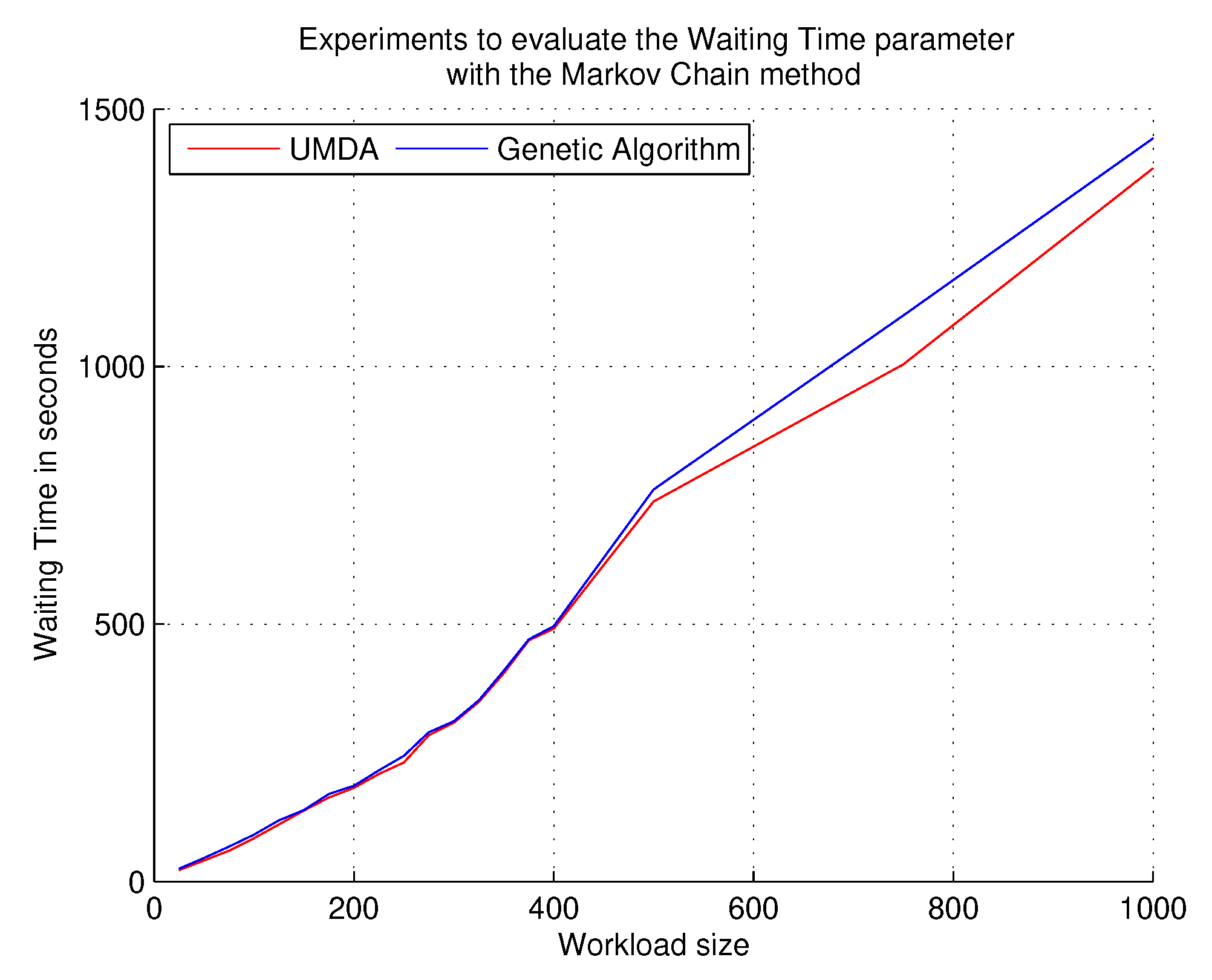
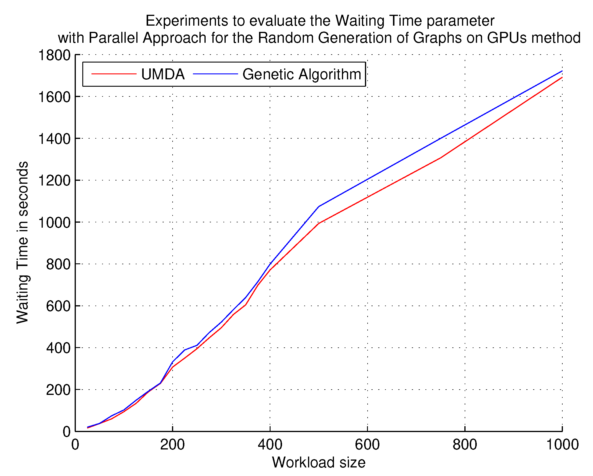
5.3. Evaluating the Waiting Time Parameter Using the Markov Chain Method and the Parallel Approach for the Random Generation of Graphs on GPUs

The evaluation parameter, waiting time, allows the observation of the time that tasks must wait before they can be served. It is an exponential parameter that increases as workloads increase the number of PTGs. The main objective of this test was to determine if the UMDA exceeds the waiting times of the genetic algorithm. The results of using the Markov Chain method and the parallel approach for the random generation of graphs on GPUs are shown in Figure 7 and Figure 8, respectively.

With both methods of synthetic load generation, the UMDA offers better waiting times; however, there was no large difference because the waiting time increased almost in the same proportion with both algorithms. The genetic algorithm produced more specific allocations in the clusters, whereas the UMDA more easily disseminated the sub-tasks in the clusters, causing waiting times to reduce during the workload increase in the experimental process.

5.4. General Comments on the Treatment of PTGs

This subsection describes the observations during the coding and testing phases of the proposed method, which may be useful for future research in the scheduling and allocation of PTGs in HDCS.

• A frequent problem in the process of PTGs is the cycles generated in the vertices; in our case, we used the deep search algorithm and obtained positive results.
• For a more realistic evaluation of PTG scheduling, it is important to consider both methods for generating synthetic workloads and loads that represent real applications.
• During the testing, it is important to have a large number of PTGs to observe the behavior of the algorithms with different workloads.

6. Discussion

In this investigation, we extended the works that consider one characteristic of the PTGs to three characteristics for their planning in the HDCS. The results of the experiments showed that using these three characteristics optimizes the allocation of the resources of the PTGs.

The results demonstrated a difference in the UMDA response speed compared to the genetic algorithm. We observed that transferring populations to a genetic representation is a considerably time-consuming process. Therefore, an evaluation was proposed that determines the quality of the assignments; this evaluation showed that the genetic algorithm can absorb a large amount of resources in each assignment. This requires new studies in the parallelization of planning as described in the next paragraph.

7. Future Work

Future work in this research could focus on two areas: method coding using parallel programming and test development in an uncontrolled environment.

With the coding of the method using parallel programming, the aim is to accelerate the execution of the programs that constitute the array method as well as to experiment with high-speed communication equipment. In this work, we also consider the speed of the processors, which is an important feature in the process of PTG allocation.

The experiments that include an uncontrolled environment are constituted by three geographically distributed clusters. A cluster, called a resident cluster, is where workloads are generated, which is then disseminated to the remaining clusters.

8. Materials and Methods

8.1. Hardware

Experiments with the array method were performed in Liebres InTELigentes cluster consisting of 3 servers configured with fedora and openSUSE Linux operating system:

• Dell EMC Power Edge Rack Server Intel Xeon generation 2 with 20 cores. Dell Technologies 701 E. Parmer Lane, Bldg PS2, Austin, TX 78753, USA.
• 2 Servers HPE ProLiant DL20 Gen10 Intel Xeon. 1501 Page Mill Rd, Palo Alto, CA 94304, USA.

Communication between servers was achieved with Switch Cisco Gigabit Ethernet SG350-28, 24 Ports 10/100/1000 Mbps. Cisco Systems, Inc. 300 East Tasman Dr. San Jose, CA 95134, USA.

8.2. Software

The Linux server was used as a resident operating system on servers. The Linux server was responsible for providing the native C language compiler. Additional libraries were installed on the servers to provide communication services in the cluster.

8.3. Method Coding

The programming language used in this research work was C using dynamic memory programming; dynamic memory allows growing and shrinking according to the requirement of synthetic workloads (it was not known how much memory was needed for the program), and memory spaces are used more efficiently.

9. Conclusions

In this study, we performed scheduling of PTGs in HDCS using three characteristics: critical path, layering, and graph density. The scheduling was performed using two separate algorithms—UMDA and genetic algorithm—to evaluate two parameters: makespan and waiting time. The tests showed that the UMDA had faster response times than the genetic algorithm in the tests proposed for this work. Both algorithms produced similar results with loads lower than 500 PTGs; with loads equal or higher than 500, the genetic algorithm had slower task allocation times in the target system. We found that the genetic algorithm looks for potentially more specific allocations in the clusters, aiming to keep the tasks closer to the allocated resources.

In addition to the tests proposed, we experimented with the quality of allocation parameter, which allowed us to count the resources that were allocated and to obtain the percentages of resources used in each allocation. This parameter allowed us to observe that the genetic algorithm improves the quality of resource allocation because it produces more combinations during the search and allocation process. Comparatively, the UMDA speeds up the allocations, but leaves resources unallocated into clusters, whereas the genetic algorithm is slow in the allocations, but optimizes the allocations of the resources available in clusters. The acceleration in the generation of allocations produced by the lack of translations make the UMDA faster in generating results, whereas the genetic algorithm is able to improve the results it provides.

Stricter testing of the allocation quality parameter will be conducted in subsequent studies.

10. Patents

This research product is being registered in the IMPI Instituto Mexicano de la Propiedad Industrial.