Article

A Finite State Method in the Performance Evaluation of the Bernoulli Serial Production Lines

Faculty of Mechanical Engineering and Naval Architecture, University of Zagreb, Ivana Lučića 5, 10000 Zagreb, Croatia
*
Author to whom correspondence should be addressed.
Appl. Sci. 2020, 10(18), 6602; https://doi.org/10.3390/app10186602
Submission received: 10 September 2020 / Revised: 18 September 2020 / Accepted: 19 September 2020 / Published: 21 September 2020
(This article belongs to the Section Mechanical Engineering)

Abstract

:
Research on the performance measure evaluation of Bernoulli serial production lines is presented in this paper. Important aspects of the modeling and analysis using transition systems within the Markovian framework are addressed, including analytical and approximation methods. The “dimensionality curse” problems of the large scale and dense transition systems in the production system engineering field are pointed out as one of the main research and development obstacles. In that respect, a new analytically-based finite state method is presented based on the proportionality property of the stationary probability distribution across the systems’ state space. Simple and differentiable expressions for the performance measures including the production rate, the work-in-process, and the probabilities of machine blockage and starvation are formulated. A finite state method’s accuracy and applicability are successfully validated by comparing the obtained results against the rigorous analytical solution.

1. Introduction

The manufacturing industry is of great importance to the national and global economies. Many historical examples, starting with the Industrial Revolution, prove that it is a path towards development and prosperity. More specifically, we have seen many times that national power correlates to control over the global manufacturing industry and means of production, like industry sectors in the US, Japan, Germany, Korea, or China. These examples prove that the growth of the manufacturing output and technological improvement boost long-term economic growth. Additionally, it is estimated that, via the multiplier effect, each manufacturing job supports 5–7 other employments in the economy across the global trade of goods and services [1]. Consequently, an efficient and sustainable economy depends on efficient and sustainable manufacturing. Given that, production system engineering (PSE) stands as a path to rationalization and improvement of the existing production systems through successful production planning and control [2].
PSE relies on production system modeling and analysis using transition system theory at different scales, and particularly on discrete timed models describing steady-state (time-invariant) and transient production system responses. Such models have been predominantly used for the performance evaluation of various serial and assembly production systems focusing on throughput, reliability, sensitivity, lead time, and bottleneck analysis, or other design and optimization problems. In addition, similar applications can be found in fields of molecular biology, evolution, healthcare, city traffic, communication services, computer algorithms, money flow, network structures, etc. [3].
The application of the stochastic modeling in the case of production systems intensified significantly in the last two decades. Currently, significant research efforts are being put into a deeper understanding of the production system behavior in the context of the internet of things [4], still strongly relying on the application of the operation research in the industrial context [5]. Therefore, a systematic approach to production system modeling using stochastic processes has great potential to contribute to current research dealing with Industry 4.0 [6] and advanced production system concepts like digital twinning [7]. In addition to that, stochastic modeling has been successfully applied in cases like tool wear condition monitoring [8], prediction of cutting force during micro-machining [9], or grinding wheel topography modeling [10]. More generally, the importance of the Markovian framework, its background, and broad application cases is proven by a quite significant number of research papers dedicated to that topic [11,12].
Concerning production system modeling, a variety of problems has been addressed in the literature, such as the performance evaluation of serial lines, assembly lines, job shops, flexible manufacturing cells, or other specific types of production. A more detailed review of different modeling approaches, including applications of the Markov processes, semi-Markov processes, queuing networks, stochastic automata networks, Petri nets, performance algebra, and diodic algebraic models, was presented recently by Papandopulos et al. [3]. It was pointed out that the majority of the research body is still dominated by the application of the Markovian framework in cases of serial production lines—“the working horse of production systems”.
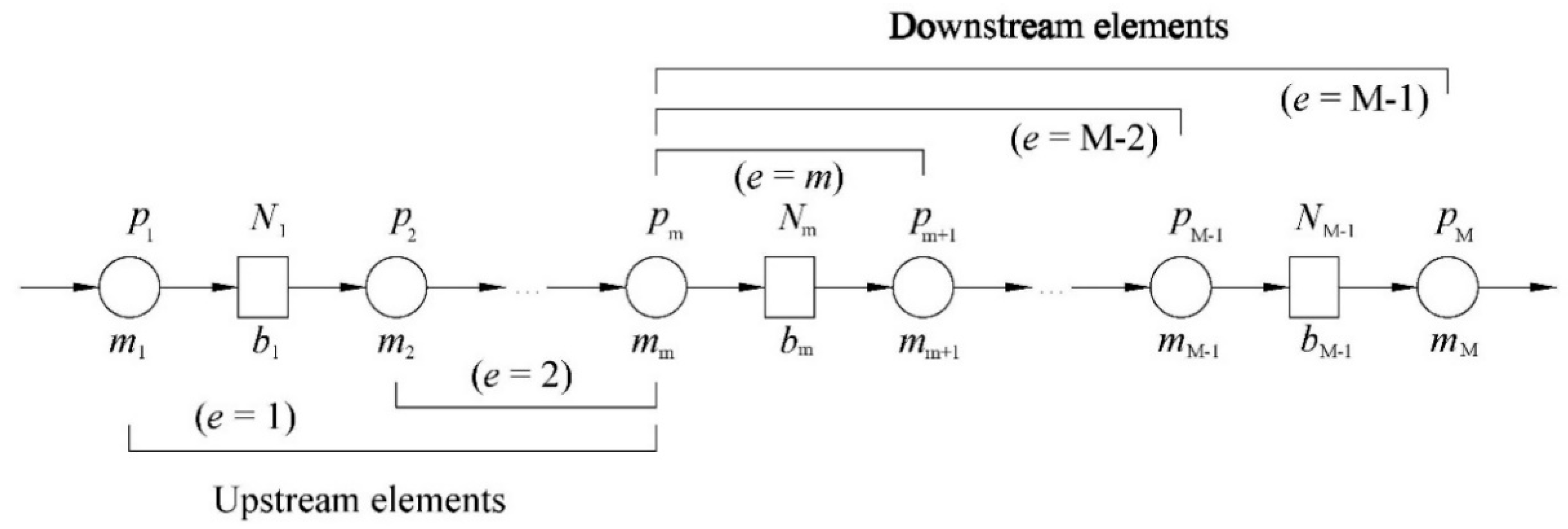
Given that, the primary goal of this paper is to present the application of the transition system theory in the case of the serial production line composed of machines and buffers of arbitrary storage capacity. Such an approach has great potential for enhancing the competitiveness and profitability of the production facilities. However, it is presently faced with a significant computational burden. This issue is bypassed by this research using Markovian modeling and the developed finite state method validated against the rigorous analytical solution to the problem.
The pioneering work on this topic was presented amid the last century by Sevast’yanov [13] who developed an analytical solution to the steady-state response of the Bernoulli serial line composed of two machines and one buffer using the integral equations. In addition, an idea of the approximation method in the case of lines with more than two machines was presented since the integral equations proved to be too complex to obtain a more general solution. The lack of the analytical solution in the case of the general Bernoulli serial line (a line with an arbitrary number of machines and buffers of arbitrary capacity) and the awareness of the “dimensionality curse” related to the large scale transition systems have motivated the researchers to further develop different approximation techniques enabling modeling and performance analysis of production systems. According to Papandopulos [3], two methods prevail, namely the decomposition and the aggregation algorithms. The first approach decomposes a production line into two pseudo-machine and one buffer sublines, while the latter uses a sequential backward–forward aggregation of two neighboring machines until a complete line is condensed into a single machine.
The advantage of the decomposition and aggregation methods is the ability to model and analyze complex production lines at low CPU (central processing unit) costs, while getting some idea of the observed production system and its properties through performance evaluation. Both methods were applied in the manufacturing industry in cases like the automotive industry, the industry of household appliances, furniture factories, etc. However, the major drawback of both methods is a lack of systematic verification against the missing analytical results. In this respect, the analytical solution of the general Bernoulli serial line problem was formulated recently using the generalized transition matrix approach [14]. Unfortunately, its application was limited due to the exponential growth of the problem scale known as the “dimensionality curse”, resulting in extensive CPU requirements and computer memory storage limitations. Consequently, the methods of approximation were verified only in a limited spectrum of problems.
However, the developed analytical solution enabled the formulation of the eigenvector associated with the largest eigenvalue of the respective transition (stochastic) matrix. Such an eigenvector can be considered as the DNA of the transition system under consideration as it is composed of the steady-state probabilities for each state of the system’s state space. This property is exploited further in the present paper in order to formulate a finite state method (FSM) that bypasses the system’s dimensionality issues and approximates the exact results. The essence of the method reflects the internal relationships between the eigenvector components, allowing further systematic verification of the approximation methods as well as research on system improvability within the Markovian framework of the serial Bernoulli production lines. The method is applied in cases of several serial Bernoulli production lines, providing a possibility of extensive verification of the aggregation method.
The remainder of the paper is structured as follows. A brief literature review is presented in the next chapter. The third chapter outlines a referent analytical solution. It also contains a detailed derivation of the FSM method as the central topic of the present research. The fourth chapter comprises a summary of the FSM validation and discussions on the obtained results. Finally, the fifth chapter presents the main conclusions of the research.

2. Brief Literature Review

Application of the Markovian modeling in the case of serial production lines has been present in the governing PSE literature body for more than 50 years, starting with the works of Sevast’yanov in 1962. However, it got broader recognition after the development of the approximation methods bridging the exponential growth of the system dimensionality issues associated with the analytical solution formulation. These approximations are usually characterized as the decomposition and the aggregation method.
The decomposition method assumes that a complete serial line can be represented by a set of two machines—one buffer line summarizing the behavior of the upstream and downstream parts of the production flow. Each of the representing lines is composed of machines with the geometric distribution of up and downtimes. The applicability of the method has been demonstrated in cases of several production lines against the performance measures obtained using simulations. In addition, a necessity for more rigorous verification against analytical results is pointed out [15]. The algorithm of the decomposition method was further improved by the evaluation number reduction [16]. An excellent and more detailed review of the decomposition method development is presented in [17]. Further application of the method in cases of the continuous flow lines composed of machines with multiple failure rates is presented in [18,19]. The decomposition approach to the problem was applied in cases of systems with closed loops, two product types, quality failures, automated lines, multiple failure modes, non-linear material flow, assembly systems, etc. [3].
The basic idea of the aggregation method is to reduce a complete production line into a single machine using an algorithm of sequential backward–forward aggregation of two adjacent machines. It was first introduced by Lim et al. [20] in research on simple and analytical modeling of traditional production lines. The method proved to be acceptably accurate and valid for application in the modern mass-production industry. Its governing feature is modeling simplicity and low computational burden. However, the method should be further verified using the analytical results as it is presently validated using extensive simulations in some selected cases [2]. Its further development comprised research in cases like production lines with quality control systems [21], improvability and bottlenecks analysis [22,23], lead time analysis [24], transient problems [25], assembly systems [26], etc.
The analytical solution of the problem is of particular significance as it enables rigorous verification of the approximation and numerical techniques, particularly in the case of decomposition and aggregation methods. Its formulation has been a known issue starting with the work of Sevast’yanov. However, it was solved recently by Hadžić [14] using the concept of the generalized transition matrix and the eigenvalue problem following [27,28]. The solution proved to be exact. However, the evaluation algorithm remained limited due to dimensionality issues. The same issue has also been addressed in [29] using the state ranking transition matrix formulation of the system for arbitrary buffer occupancy and corresponding outcome states.
The “dimensionality curse” problems of the large scale and dense transition systems are present across different scientific disciplines. Consequently, researchers make significant efforts to develop various interpretation algorithms capable of cracking problems into simpler forms while keeping the original state-time framework [30]. Some of the possibilities include external memory storages (storing complete transition matrix), selective matrix criteria, lumping states according to the model properties, and sparse matrix approximation [31]. Additionally, the PSE research community investigated this issue intensively. The development of different approaches and algorithms includes methods for the specification of the system and numerical solution methods. In the first case, the governing research comprises Kronecker and tensor algebra, hierarchical modeling, complex analysis, and other approaches. The main topics in the latter case cover direct, iterative and sparse matrix methods, separable preconditioning, explicit storage algorithms, parallel computing techniques, etc. One of the main drawbacks of these methods is a requirement of compatibility between methods for system specification and the numerical solution of the problem [3].

3. Mathematical Modeling

3.1. Analytical Solution

Consider a serial production line composed of M machines mi, i = 1, 2, …, M of the Bernoulli(pi) reliability model, where pi is the probability of machine being in state {up}, Figure 1. In addition, consider a series of buffers bi, i = 1, 2, …, M-1 of capacity Ni 0, where 0 denotes the set of natural numbers. Each buffer is placed in between two adjacent machines. Assume that (a) the machine status does not depend on the status of other machines, (b) the time axis is slotted and machines begin operations at the beginning of each slot, (c) machines’ and buffers’ statuses are determined at the beginning of each slot, (d) the machines have an identical cycle time, and (e) the first machine is never starved and the last one is never blocked [2].
The behavior of such a system can be modeled using stochastic processes. More specifically, it can be modeled as the discrete-time Markov chain {Xn, n = 0, 1, 2, …} over the system’s state space S defined according to the buffers’ capacities, Figure 1. More specifically, each state in the system’s state space represents one possible combination of buffer occupancies. The transition of the system from one state to another is described using transition probabilities, [P(p1,p2,…pM)], also known as the transition matrix, which can be expressed as:
[ P ( p 1 , p 2 , p M ) ] = [ P 1 ( p 1 ) ] [ P 2 ( p 2 ) ] [ P 3 ( p 3 ) ] [ P M ( p M ) ] = i = 1 M [ P i ( p i ) ] .
A detailed formulation of the transition probabilities using the generalized transition matrix concept and constitutive matrices [Pi(pi)] are available in [14]. The system in hand is a finite, irreducible, and aperiodic Markov chain. Hence, a solution to the Chapman–Kolmogorov equations is the eigenvector associated with the largest eigenvalue of the transition matrix. Such an eigenvector represents a limiting distribution that is identical to the stationary distribution of the Markov chain [32,33]. The stationary distribution of the Markov chain is of great significance for the performance evaluation. It can, therefore, be considered as the DNA of the production line, or more generally of the production system. It is also fundamental for the FSM derivation and validation of the existing approximation techniques.

3.2. A Finite State Method

Let us first take a look at the properties of a stationary distribution (eigenvector associated with the eigenvalue equal to 1) in the case of a three-machine line with arbitrary properties. Limitation to the case of a three-machine line of specific properties will be used here without loss of generality to illustrate the basic property of the stationary distribution. A similar conclusion can be drawn if a different arrangement of the line or a line with another number of machines is considered. Therefore, assume for simplicity that p1 = 0.6, p2 = 0.7, and p3 = 0.8, and that N1 = N2 = 10, Figure 2a. The corresponding stationary distribution can be calculated without significant efforts using the analytical approach [14]. The obtained distribution of the stationary probabilities across the state space of the Bernoulli serial line is presented in Figure 2b including (N1 + 1) × (N2 + 1) = 121 possible system states. Proportional relationships between stationary probabilities of the considered system can easily be detected. Moreover, it turns out that such proportionality is a common property of Markov chains describing the behavior of the serial Bernoulli production lines. This property is used as the basis to develop FSM as an analytically-based method capable of breaking the dimensionality issues.
The eigenvector of the considered three-machine line (see Figure 2) can be decomposed into two classes of states. State 0 and states which are a multiple of N1 + 1 = 11 stand for combinations of buffer occupancy N1 = N2 = 0, N1 = 1 and N2 = 0, N1 = 2 and N2 = 0, ..., N1 = 10 and N2 = 0. These combinations represent the external class of the states. States between 0 and 11, as well as states between multiples of N1 + 1 = 11 cover combinations N1 = 0 and N2 = 1, N1 = 0 and N2 = 2, …, N1 = 0 and N2 = 10, N1 = 1 and N2=1, …, N1 = 10 and N2 = 10. These combinations stand for the internal class of the states. Further analysis of the considered problem reveals that the proportional relationship between the states in the external class is governed by the stationary probability distribution determined analytically in the case of a two-machine line: p1-N1-p2. Similarly, the proportional relationship between the states in the internal class is governed by the stationary probability distribution determined analytically in the case of a two-machine line: p1-N2-p3. Therefore, the corresponding eigenvector can be determined using the well-known and simple analytical solution of the two-machine line problem [2] at considerably lower CPU and memory storage costs using two finite state elements: p1-N1-p2 and p1-N2-p3. Notice that p1 is a common property of both elements and also that p1=min{ p1, p2, p3}.
Let us now consider a general case of the serial Bernoulli production line (see Figure 3) with a machine m, pm = min{pi}, i = 1, 2, …, M. It is clear that there is a total number of m − 1 upstream and Mm downstream machines. Define M − 1 finite state elements, (e), such that a complete line is replaced by a set of pe-Ne-pm upstream and pm-Ne-pe+1 downstream elements.
More specifically, the stationary distributions of the upstream elements are equal to:
P ( e ) T = P 0 ( e ) P 1 ( e ) P 2 ( e ) P N e ( e ) T = P i e ( e ) T ,
where ie = 0, 1, 2, …, Ne stands for state on the buffer of the element e = 1, 2, …, m − 1. The pertaining probabilities can be determined using the analytical solution in the case of a line composed of two machines and one buffer [2]:
P 0 ( e ) = ( 1 p e ) ( 1 α e ) 1 p e p m α e N e ,   α e = p e ( 1 p m ) p m ( 1 p e ) ,   P i e ( e ) = α e i e 1 p m P 0 ( e ) .
Similarly, the stationary distributions of the downstream elements can be determined using:
P 0 ( e ) = ( 1 p m ) ( 1 α e ) 1 p m p e + 1 α e N e ,   α e = p m ( 1 p e + 1 ) p e + 1 ( 1 p m ) ,   P i e ( e ) = α e i e 1 p e + 1 P 0 ( e ) ,
where e = m, m + 1, …, M − 1. The eigenvector representation of the stationary distribution is the same as in the upstream case, Equation (2). The application of Equations (2)–(4) results in a total number of M − 1 stationary distributions (elementary eigenvectors) that can be used to formulate the stationary distribution (eigenvector) of the complete serial line covering all of the considered system states without loss of generality. The application of the proportional relationships within the state space of the considered transition system yields a general component of the stationary distribution (i.e., the probability that buffers of the system are in state i1, i2, …, iM − 1), P i 1 i 2 i 3 i M 1 , expressed as:
P i 1 i 2 i 3 i M 1 = P 000 0 P i 1 ( 1 ) P 0 ( 1 ) P i 2 ( 2 ) P 0 ( 2 ) P i 3 ( 3 ) P 0 ( 3 ) P i M 1 ( M 1 ) P 0 ( M 1 ) = P 000 0 e = 1 M 1 P i e ( e ) P 0 ( e ) .
The unknown P 000 0 state of the system (all buffers are empty) from Equation (5) can be determined using the well-known condition i 1 = 0 N 1 i 2 = 0 N 2 i 3 = 0 N 3 i M 1 = 0 N M 1 P i 1 i 2 i 3 i M 1 = 1 , i.e., it follows that:
P 000 0 = 1 i 1 = 0 N 1 P i 1 ( 1 ) P 0 ( 1 ) i 2 = 0 N 2 P i 2 ( 2 ) P 0 ( 2 ) i 3 = 0 N 3 P i 3 ( 3 ) P 0 ( 3 ) i M 1 = 0 N M 1 P i M 1 ( M 1 ) P 0 ( M 1 ) .
Equation (6) can be modified by extracting 1 / P 0 ( e ) in the denominator yielding:
P 000 0 = 1 1 P 0 ( 1 ) i 1 = 0 N 1 P i 1 ( 1 ) 1 P 0 ( 2 ) i 2 = 0 N 2 P i 2 ( 2 ) 1 P 0 ( 3 ) i 3 = 0 N 3 P i 3 ( 3 ) 1 P 0 ( M 1 ) i M 1 = 0 N M 1 P i M 1 ( M 1 ) .
Since i e N e P i e ( e ) = 1 , the Equation (7) is simplified into the form:
P 000 0 = P 0 ( 1 ) P 0 ( 2 ) P 0 ( 3 ) P 0 ( M 1 ) = e = 1 M 1 P 0 ( e ) .

3.3. Performance Measures

Performance measures are of particular interest for the PSE and Markov chain framework. It is, therefore, of great significance to develop simple expressions for the production rate (PR), work-in-process (WIP) for each buffer, as well as the probabilities of blockage (BL) and starvation (ST) for each machine [2]. The production rate, PR, is the average number of parts produced by the last machine of the production line. Therefore, it is an intersection of events { m M   is   in   state   up } and { b M 1   is   not   empty } , i.e.:
P R = P ( { m M   is   in   state   up } { b M 1   is   not   empty } ) .
Equation (9) can be expressed using the stationary distribution as:
P R = p M ( 1 i 1 = 0 N 1 i 2 = 0 N 2 i 3 = 0 N 3 i M 2 = 0 N M 2 P i 1 i 2 i 3 i M 2 0 ) .
By applying Equation (5), the production rate can be formulated in terms of the finite state elements as:
P R = p M [ 1 P 000 0 i 1 = 0 N 1 i 2 = 0 N 2 i 3 = 0 N 3 i M 2 = 0 N M 2 ( e = 1 M 2 P i e ( e ) P 0 ( e ) ) ] .
Substitution of Equation (8) into Equation (11) yields:
P R = p M [ 1 P 0 ( 1 ) P 0 ( 2 ) P 0 ( M 1 ) ( P 0 ( 1 ) P 0 ( 1 ) + P 1 ( 1 ) P 0 ( 1 ) + + P N 1 ( 1 ) P 0 ( 1 ) ) ( P 0 ( 2 ) P 0 ( 2 ) + P 1 ( 2 ) P 0 ( 2 ) + + P N 2 ( 2 ) P 0 ( 2 ) ) ( P 0 ( M 2 ) P 0 ( M 2 ) + P 1 ( M 2 ) P 0 ( M 2 ) + + P N 2 ( M 2 ) P 0 ( M 2 ) ) ] ,
which can be simplified using a relation i e N e P i e ( e ) = 1 to the form:
P R = p M [ 1 P 0 ( M 1 ) ] .
Therefore, the production rate can be expressed simply in terms of the probability of the state {up} of the last machine, pM, and the first component of the elementary eigenvector obtained using the pm-NM−1-pM element.
Similarly, the work-in-process as the average number of parts contained at buffer bi is equal to:
W I P i = W I P e = i 1 = 0 N 1 i 2 = 0 N 2 i 3 = 0 N 3 i M 1 = 0 N M 1 i e P i 1 i 2 i 3 i M 1 .
Again, using Equation (5), the work-in-process can be expressed as:
W I P e = P 000 0 i 1 = 0 N 1 i 2 = 0 N 2 i 3 = 0 N 3 i M 1 = 0 N M 1 ( i e e = 1 M 1 P i e ( e ) P 0 ( e ) ) .
Substitution of Equation (8) into Equation (15) after algebraic manipulation and by using identity i e N e P i e ( e ) = 1 yields:
W I P e = i e = 0 N e i e P i e ( e ) = W I P i .
Consequently, the work-in-process associated with the ith buffer depends solely on the elementary eigenvector { P ( e ) } obtained using the corresponding finite state element.
A machine blockage is commonly formulated using union and intersections of several events, i.e.:
B L i = P ( { m i   is   up } { m i + 1   is   down } { b i   is   full } ) + P ( { m i   is   up } { b i   is   full } ) B L i + 1 .
The probability of blockage, BLi, of the machine mi, Equation (17), can be expressed using the finite state elements as:
B L i = p i ( 1 p i + 1 + B L i + 1 ) i 1 = 0 N 1 i 2 = 0 N 2 i 3 = 0 N 3 i M 1 = 0 N M 1 P i 1 i 2 i 3 ( i e = N e ) i M 1 ,
which after inserting Equations (5) and (8), yields:
B L i = p i ( 1 p i + 1 + B L i + 1 ) P N e ( e = i ) .
Since the last machine can never be blocked, i.e., BLM = 0, the probability of the blockage of the penultimate machine equals:
B L M 1 = p M 1 ( 1 p M ) P N e ( M 1 ) .
The probability of starvation, STi, of the machine mi can be determined using the intersection of events:
S T i = P ( { m i   in   state   up } { b i 1   is   empty } ) .
Using the finite state elements, Equation (20) can be formulated as:
S T i = p i i 1 = 0 N 1 i 2 = 0 N 2 i 3 = 0 N 3 i M 1 = 0 N M 1 P i 1 i 2 i 3 ( i e = 0 ) i M 1 .
Again, using Equations (5) and (8), the probability of starvation of the ith machine is equal to:
S T i = p i P 0 ( e = i 1 ) .
As the first machine cannot be starved, the probability of starvation of the machine m1 takes a zero value.
Finally, it is important to point out that a complete reconstruction of the stationary distribution of the considered line is not necessary. It is sufficient to evaluate only the stationary distributions at the finite state element level and to collect the first and the last components to determine the production rate as well as the probabilities of blockage and starvation. Evaluation of the work-in-process, however, requires more detailed data on all components of the considered finite state element. The FSM approach is, therefore, very convenient for practical and daily factory-floor applications.

4. Validation and Application of the Developed Theory

Validation of the developed FSM is performed in cases of the serial Bernoulli lines L1–L9 with probabilities of the state {up} specified in Table 1. Performance measures were calculated using Equations (12), (15), (18), (19) and (22) for each line using the analytical solution (AN), the aggregation procedure (AGG) and the FSM using ProLab, an in-house software developed by the authors, and PSEToolbox (Production System Engineering Toolbox) [2]. Evaluation of the performance measures was performed for the specified lines as well as for their permutations including even and uneven distribution of the buffer occupancy. However, only selected and the most interesting results are presented here. In addition, to enable a simple graphical presentation of the results, all of the buffer occupancies were selected as fractions or multiplies of the first or the last buffer’s capacity. Nevertheless, the considered approach was valid in case of the arbitrary buffer occupancies. Buffer occupancy was specified separately for each considered case.
As the first step of the FSM validation, a line L1 was considered to check the fundamental accuracy of the method against the well known analytical solution of the line composed of two machines and one buffer. The performance measured in the case of the line L1 and its reverse were evaluated using AN, AGG, and FSM approaches and are compared in Figure 4 and Figure 5. Both AGG and FSM approaches agreed very well with the analytical results in this simplest case, except for some negligible discrepancies due to numerical reasons. An excellent agreement could also be noticed in the asymptotic values approached by the performance curves in all three cases. In addition, a reversibility property of the line was excerpted nicely.
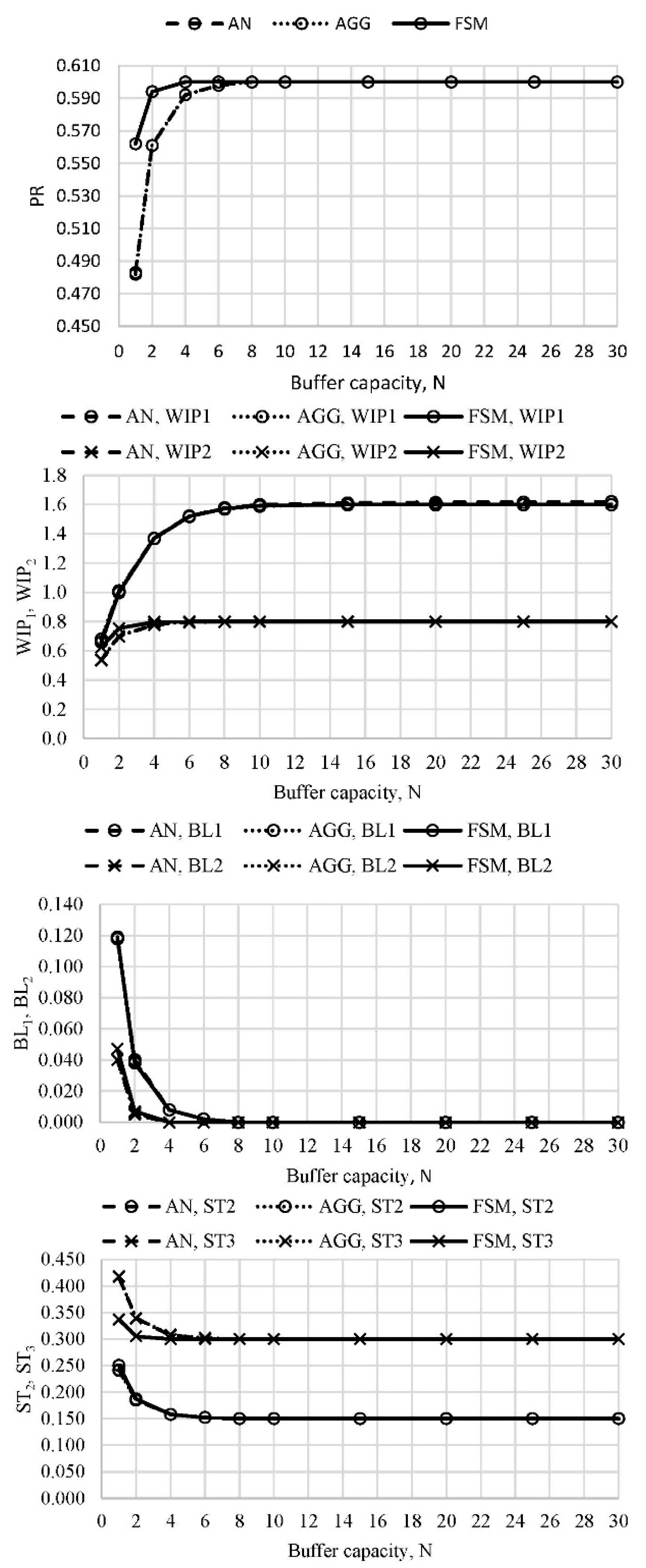
The performance measures of the line with three machines were evaluated in several cases. The first case, L2, took into account the original arrangement of machines (see Table 1) and even buffer capacity distribution along the line. Figure 6 presents the distribution of the performance measures as a function of buffer capacity. A good agreement of both AGG and FSM with the analytical results was evident, except for slight discrepancies in PR and ST3 between AN and FSM solution for the lowest level of buffers’ capacity.
Uneven distribution of the buffer capacity and perturbed arrangement of the machines were evaluated in the case of the line labeled as L2′. The third case, L2′R, considered a reverse of the L2′ line. The performance measures obtained using AN, AGG, and FSM approaches are presented in Figure 7 and Figure 8 as functions of the buffer capacity. It can be seen that generally, all three methods agreed well, particularly in asymptotic values of the performance measures. It can also be noticed that the reversibility property held for lines L2′ and L2′R.
Performance measures of the line with four machines were evaluated in three cases of different machine arrangements including the uneven distribution of the buffer capacity. A comparison between the obtained results is presented in Figure 9, Figure 10 and Figure 11 in cases of lines L3A, L3B, and L3C. Again, the discrepancies were related to the smallest state spaces of buffers with small capacity. As the state space increased, the methods approached the same asymptotic values. It is interesting to notice a relationship between the position of the worst machine, WIP, BL, and ST. In a case when the worst machine was in position i = 2, 3, …, M, WIPi−1 altered from the asymptotic function to an almost linear curve, while BLi−1 and STi altered pertaining asymptotes.
The above examples proved a quite good agreement between the aggregation procedure, the finite state method, and the analytical solution. Therefore, the analytical solution could be omitted from further evaluations of lines L4–L9 as it would require considerably more CPU time as compared to the AGG and FSM algorithms. Further, to avoid the presentation of extensive data generated by the evaluation, only asymptotic values of the performance measures of lines L4–L9 are presented in Figure 12 and Figure 13. The machine arrangement is presented in Table 1, while the buffer occupancy is considered to be even along the lines. The obtained asymptotic value of the production rate was, as expected, the same for both lines and was equal to 0.6. The probability of machine blockage was also equal to 0 since the first machine was also the worst one. The asymptotic values of the work-in-process for each buffer of lines L4–L9 are presented in Figure 12. It can be seen that both methods yielded almost the same values. Additionally, the asymptotic values of the probability of starvation for each machine of the considered lines are presented in Figure 13. A nice agreement between the results can be noticed.

Discussion

Three different methods were considered in the research: The analytical solution, the aggregation procedure, and the newly developed finite state method. Both approximation methods demonstrated respectable accuracy as compared to the analytical results. Therefore, both the AGG and the FSM approaches could be recommended for further application for the performance evaluation of the serial Bernoulli production line. This also includes the decomposition method since it was already verified successfully against the aggregation method [34].
Some drawbacks of the FSM as compared to the aggregation algorithm manifest in the range of the small buffer occupancy due to relatively rough system state discretization using the finite elements. This drawback is more pronounced as the probabilities pi approach the same value. However, this issue diminishes with the augmentation of the state space. The presented FSM was a powerful and analytically-based tool that enabled validation of the aggregation and decomposition procedure in complex cases that were previously unreachable to the conventional analytical approach. Its CPU requirements were comparable to other approximation algorithms, while the analytical approach remained an extremely CPU-demanding approach. Additional advantages of the FSM in comparison to other approximation methods are the differentiability and reconstruction of the production system eigenvector. The differentiability is of great significance in the field of improvement of production lines. This feature was enabled by the FSM since the performance measures were analytically related to the governing line properties. Additionally, the reconstruction of the system’s stationary probability distribution vector (eigenvector) was of great value to the researcher in the PSE field as it enabled a deeper understanding of the behavior of complex production systems.

5. Conclusions

Manufacturing is of great importance for the global economy and society. It is, therefore, of great significance to master the analysis and design of various production systems. In that respect, research on the performance measures evaluation of the Bernoulli serial production lines was presented in this paper. Several important aspects of the modeling and analysis using transition systems within the Markovian framework were addressed, including analytical and approximation methods. The “dimensionality curse” problems of the large scale and dense transition systems in the PSE field were pointed out as one of the main research and development obstacles.
Given that, a new analytically-based FSM approach was developed based on the proportionality property of the stationary probability distribution across the systems’ state space. An analytical solution of the two machine-one buffer line was exploited to formulate finite state elements used to model a complete Bernoulli serial production line. Simple and differentiable expressions for the performance measures including the production rate, the work-in-process, and the probabilities of machine blockage and starvation were developed. The FSM accuracy and applicability were successfully validated by comparing the obtained results against the rigorous analytical solution. In addition to that, a thorough validation of the aggregation method was provided, proving its accuracy and applicability. Currently, the FSM is limited to the evaluation of the single product lines as the cycle time was assumed to be equal at each machine along the line. Other limitations are related to the assumption of a Bernoulli reliability model of each machine along the line as well as to the assumption of occurrence of the machine breakdowns and repairs at the beginning of each cycle which may not be in complete agreement with the real production system.
Further research in the PSE field, as well as further development and application of the FSM, should focus on the analytical formulation of problems like improvability analysis, design of lean production lines, closed Bernoulli lines, Bernoulli lines with rework, assembly systems, the steady-state and transient behavior of transition systems, etc. Additionally, further effort should be put into FSM modeling of the production lines involving multiple products of different processing times. Such research will make it possible to model complex stochastic relationships in cases of systems like ship production or other job shop production systems. A significant impact on the PSE research body would also be accomplished in case of validation of the evaluation methods against the factory floor data. Last but not the least, it would be interesting to research a possibility to apply the FSM approach in cases of other large scale transition systems typically encountered in fields of physics, biology, chemistry, ecology, etc.

Author Contributions

Conceptualization, N.H.; methodology, N.H.; software, N.H.; validation, V.L. and F.A.; formal analysis, V.L.; investigation, N.H.; resources, N.H.; writing—original draft preparation, N.H. and V.L.; writing—review and editing, V.L. and F.A.; visualization, N.H.; supervision, N.H.; project administration, N.H.; funding acquisition, N.H. All authors have read and agreed to the published version of the manuscript.

Funding

The research was supported by the Croatian Science Foundation, project UIP-2019-04-6573 ANTYARD (Advanced Methodologies for Cost-Effective, Energy Efficient, and Environmentally Friendly Ship Production Process Design) and by the University of Zagreb, project Multicriterial Mathematical Models for Design and Construction of Ships.

Conflicts of Interest

The authors declare no conflict of interest.

Abbreviations

AGGAGGregation procedure
ANAnalytical solution
CPUCentral processing unit
DNADeoxyriboNucleic acid
FSMFinite state method
PSEProduction system engineering

References

  1. Bivens, J. Updated Employment Multipliers for the U.S. Economy; Economic Policy Institute: Washington, DC, USA, 2019. [Google Scholar]
  2. Li, J.; Meerkov, S.M. Production System Engineering; Springer: New York, NY, USA, 2009. [Google Scholar]
  3. Papadopoulos, C.T.; Li, J.; O’Kelly, M.E.J. A classification and review of timed Markov models of manufacturing systems. Comput. Ind. Eng. 2019, 128, 219–244. [Google Scholar] [CrossRef]
  4. Wang, J.; Ma, Y.; Zhang, L.; Gao, R.X.; Wu, D. Deep learning for smart manufacturing: Methods and applications. J. Manuf. Syst. 2018, 48, 144–156. [Google Scholar] [CrossRef]
  5. Napoleone, A.; Macchi, M.; Pozzetti, A. A review on the characteristics of cyber-physical systems for the future smart factories. J. Manuf. Syst. 2020, 54, 305–335. [Google Scholar] [CrossRef]
  6. Grznár, P.; Gregor, M.; Krajčovič, M.; Mozol, Š.; Schickerle, M.; Vavrík, V.; Ďurica, L.; Marschall, M.; Bielik, T. Modeling and Simulation of Processes in a Factory of the Future. Appl. Sci. 2020, 10, 4503. [Google Scholar] [CrossRef]
  7. Wärmefjord, K.; Söderberg, R.; Schleich, B.; Wang, H. Digital Twin for Variation Management: A General Framework and Identification of Industrial Challenges Related to the Implementation. Appl. Sci. 2020, 10, 3342. [Google Scholar] [CrossRef]
  8. Ertunc, H.M.; Loparo, K.A.; Ocak, H. Tool wear condition monitoring in drilling operations using hidden Markov models (HMMs). Int. J. Mach. Tools Manuf. 2001, 41, 1363–1384. [Google Scholar] [CrossRef]
  9. Aly, M.; Ng, E.; Veldhuis, S.; Elbestawi, M. Prediction of cutting forces in the micro-machining of silicon using a “hybrid molecular dynamic-finite element analysis” force model. Int. J. Mach. Tools Manuf. 2006, 46, 1727–1739. [Google Scholar] [CrossRef]
  10. Doman, D.A.; Warkentin, A.; Bauer, R. A survey of recent grinding wheel topography models. Int. J. Mach. Tools Manuf. 2006, 46, 343–352. [Google Scholar] [CrossRef]
  11. Bielecki, T.R.; Jakubowski, J.; Niewęgłowski, M. Conditional Markov chains: Properties, construction and structured dependence. Stoch. Process Appl. 2017, 127, 1125–1170. [Google Scholar] [CrossRef] [Green Version]
  12. El Machkouri, M.; Jakubowski, A.; Volnỳ, D. Stable limits for Markov chains via the Principle of Conditioning. Stoch. Process. Appl. 2020, 130, 1853–1878. [Google Scholar] [CrossRef] [Green Version]
  13. Sevast’yanov, B.A. Influence of Storage Bi Capacity on the Average Standstill Time of Production Line. Theory Probab. Appl. 1962, 7, 429–438. [Google Scholar] [CrossRef]
  14. Hadžić, N. Analytical Solution of the serial Bernoulli production line steady-state performance and its application in the shipbuilding process. Int. J. Prod. Res. 2018, 57, 1052–1065. [Google Scholar] [CrossRef]
  15. Gershwin, S.B. An Efficient Decomposition Method for the Approximate Evaluation of Tandem Queues with Finite Storage Space and Blocking. Oper. Res. 1987, 35, 291–305. [Google Scholar] [CrossRef]
  16. Dallery, Y.; David, R.; Xie, X.-L. An Efficient Algorithm for Analysis of Transfer Lines With Unreliable Machines and Finite Buffers. IIE Trans. 1988, 20, 280–283. [Google Scholar] [CrossRef]
  17. Dallery, Y.; Gershwin, S.B. Manufacturing flow line systems: A review of models and analytical results. Queueing Syst. 1992, 12, 3–94. [Google Scholar] [CrossRef] [Green Version]
  18. Tan, B.; Gershwin, S.B.; Tan, B. Analysis of a general Markovian two-stage continuous-flow production system with a finite buffer. Int. J. Prod. Econ. 2009, 120, 327–339. [Google Scholar] [CrossRef] [Green Version]
  19. Tan, B.; Gershwin, S.B. Modelling and analysis of Markovian continuous flow systems with a finite buffer. Ann. Oper. Res. 2009, 182, 5–30. [Google Scholar] [CrossRef]
  20. Lim, J.-T.; Meerkov, S.; Top, F. Homogeneous, asymptotically reliable serial production lines: Theory and a case study. IEEE Trans. Autom. Control 1990, 35, 524–534. [Google Scholar] [CrossRef]
  21. Jacobs, D.; Meerkov, S.M. Asymptotically reliable serial production lines with a quality control system. Comput. Math. Appl. 1991, 21, 85–90. [Google Scholar] [CrossRef] [Green Version]
  22. Jacobs, D.; Meerkov, S.M. A system-theoretic property of serial production lines: Improvability. Int. J. Syst. Sci. 1995, 26, 755–785. [Google Scholar] [CrossRef]
  23. Chiang, S.-Y.; Kuo, C.-T.; Meerkov, S.M. c-Bottlenecks in serial production lines: Identification and application. Math. Probl. Eng. 2001, 7, 543–578. [Google Scholar] [CrossRef]
  24. Meerkov, S.M.; Yan, C.-B. Production Lead Time in Serial Lines: Evaluation, Analysis, and Control. IEEE Trans. Autom. Sci. Eng. 2016, 13, 663–675. [Google Scholar] [CrossRef]
  25. Chen, G.; Wang, C.; Zhang, L.; Arinez, J.; Xiao, G. Transient Performance Analysis of Serial Production Lines With Geometric Machines. IEEE Trans. Autom. Control 2015, 61, 877–891. [Google Scholar] [CrossRef]
  26. Chiang, S.-Y.; Kuo, C.-T.; Lim, J.-T.; Meerkov, S.M. Improvability of assembly systems I: Problem formulation and performance evaluation. Math. Probl. Eng. 2000, 6, 321–357. [Google Scholar] [CrossRef] [Green Version]
  27. Hadžić, N.; Tomić, M.; Matić, S. Analytical and numerical methods in ship production engineering. In Proceedings of the XXII Symposium SORTA 2016, Trogir, Croatia, 6–8 October 2016. [Google Scholar]
  28. Hadžić, N.; Tomić, M. Analytical solution of steady-state behavior of Bernoulli production line with two finite buffers. Brodogradnja 2017, 68, 85–102. [Google Scholar] [CrossRef]
  29. Zhang, L.; Wang, C.; Arinez, J.; Biller, S. Transient analysis of Bernoulli serial lines: Performance evaluation and system-theoretic properties. IIE Trans. 2013, 45, 528–543. [Google Scholar] [CrossRef]
  30. Schapaugh, A.; Tyre, A.J. A simple method for dealing with large state spaces. Methods Ecol. Evol. 2012, 3, 949–957. [Google Scholar] [CrossRef]
  31. Reichel, K.; Bahier, V.; Midoux, C.; Parisey, N.; Masson, J.-P.; Stoeckel, S. Interpretation and approximation tools for big, dense Markov chain transition matrices in population genetics. Algorithms Mol. Biol. 2015, 10, 31. [Google Scholar] [CrossRef]
  32. Kulkarni, V.G. Introduction to Modeling and Analysis of Stochastic Systems; Springer: New York, NY, USA, 2011. [Google Scholar]
  33. Pishro-Nik, H. Introduction to Probability, Statistics, and Random Processes; Kappa Research LCC: San Bernardino, CA, USA, 2014. [Google Scholar]
  34. Li, J.; Blumenfeld, D.E.; Alden, J.M. Comparisons of two-machine line models in throughput analysis. Int. J. Prod. Res. 2006, 44, 1375–1398. [Google Scholar] [CrossRef]
Figure 1. A model of the serial production line including M machines and M-1 buffers with pertaining state space (authors’ work).
Applsci 10 06602 g001
Figure 2. (a) The considered Bernoulli serial line (p1 = 0.6, p2 = 0.7, p3 = 0.8, N1 = N2 = 10) including the pertaining state space and (b) the distribution of the stationary probabilities across the state space (authors’ work).
Applsci 10 06602 g002
Figure 3. A general case of the serial Bernoulli production line and finite state elements (authors’ work).
Applsci 10 06602 g003
Figure 4. PR, WIP, BL1, and ST2 in case of the line L1 (authors’ work).
Applsci 10 06602 g004
Figure 5. PR, WIP, BL1, and ST2 in case of the line L1R (authors’ work).
Applsci 10 06602 g005
Figure 6. PR, WIP1, WIP2, BL1, BL2, ST2, and ST3 in case of the line L2, N1 = N2 = N (authors’ work).
Applsci 10 06602 g006
Figure 7. Performance measures of the perturbed line L2′ (N1 = N, N2 = ½N1) (authors’ work).
Applsci 10 06602 g007
Figure 8. Performance measures of the perturbed line L2′R (N1 = ½N2, N2 = N) (authors’ work).
Applsci 10 06602 g008
Figure 9. Performance measures of the line L3A (N1 = N, N2 = 2N, N3 = N) (authors’ work).
Applsci 10 06602 g009
Figure 10. Performance measures of the line L3B (N1 = N, N2 = 2N, N3 = N) (authors’ work).
Applsci 10 06602 g010
Figure 11. Performance measures of the line L3C (N1 = N, N2 = 2N, N3 = N) (authors’ work).
Applsci 10 06602 g011
Figure 12. Asymptotic occupancies of buffers, lines L4–L9 (authors’ work).
Applsci 10 06602 g012
Figure 13. Asymptotic probability of the starvation, lines L4–L9 (authors’ work).
Applsci 10 06602 g013
Table 1. List of considered serial Bernoulli production lines with probabilities of the state {up} (authors’ work).
LineMp1p2p3p4p5p6p7p8p9p10
L120.60.9
L1R20.90.6
L230.60.750.9
L2′30.60.750.9
L2′R30.90.750.6
L3A40.60.70.80.9
L3B40.70.60.80.9
L3C40.90.70.60.8
L450.60.6750.750.8250.9
L560.60.660.720.780.840.9
L670.60.650.70.750.80.850.9
L780.60.6430.6860.7290.7720.8150.8580.9
L890.60.6370.6740.7110.750.7870.8240.8620.9
L9100.60.6330.6660.6990.7320.7650.7980.8310.8640.9

