Article

Characteristic Analysis and Co-Validation of Hydro-Mechanical Continuously Variable Transmission Based on the Wheel Loader

1
College of Mechanical and Electronic Engineering, Shandong University of Science and Technology, Qingdao 266590, China
2
Department of Mechanical Design and Manufacturing, College of Mechanical and Architectural Engineering, Taishan University, Taian 271000, China
*
Author to whom correspondence should be addressed.
Appl. Sci. 2020, 10(17), 5900; https://doi.org/10.3390/app10175900
Submission received: 28 June 2020 / Revised: 22 August 2020 / Accepted: 24 August 2020 / Published: 26 August 2020
(This article belongs to the Special Issue Advanced Engine Technologies and Innovative Vehicle Driving Systems)

Abstract

:
Energy-saving and emission reduction has become the theme of the world. The wheel loader has a harsh working environment, complicated working conditions, and drastic changes in load, and the performance of the engine cannot be fully utilized. Therefore, the variable speed transmission of vehicles plays a vital role in improving the efficiency and performance of the vehicle. This paper establishes the general characteristic equations for the input coupling type of hydro-mechanical continuously variable transmission (HMCVT) based on the wheel loader and determines reasonable structural forms for connection of working conditions. It establishes the general efficiency equation for the reasonable structural form for efficiency analysis and presents a method of co-validation of the simulation and test for making the results of efficiency more accurate. Through this method, the transmission performance is more accurately analyzed, which provides an important guiding role and validation for the early design of HMCVT. Eventually, it gets reasonably optimized products and reduces the design cost and cycle.

1. Introduction

The wheel loader, as a kind of off-highway vehicle, has complicated working conditions and drastic changes in load. Hence, the vehicle’s transmission plays a vital role in improving its efficiency and performance. The conventional transmission applied to the wheel loader is the mechanical transmission with torque converter. Therefore, many scholars have studied the traditional transmission with torque converter [1,2,3]. However, the efficiency of the torque converter has a greater impact on the efficiency of the transmission system, which results in no significant increase in efficiency, whatever structure is adopted. Therefore, the hydro-mechanical continuously variable transmission (HMCVT) has received widespread attention. Hydro-mechanical continuously variable transmission (HMCVT) is a kind of power split transmission. Composition of the HMCVT is as displayed in Figure 1. The input power is divided into two paths (mechanical transmission and hydrostatic CVT) through the power split device, and the power of the two paths will be combined through the power junction device (PJD). It can achieve high-efficiency power transmission through mechanical transmission and CVT through hydrostatic transmission.
The efficiency of the hydrostatic transmission is higher than the hydrodynamic transmission. The hydrostatic transmission not only has high efficiency compared to the hydrodynamic transmission, but also can achieve CVT and has the adaptability to the load. Many companies like Dana Rexroth, ZF, and Liebherr, have developed and produced HMCVT, and the efficiency has generally improved by about 25% [4,5,6,7]. Many scholars have studied hydrostatic mechanical power split transmission. Ince et al. developed a novel power-split-input-coupled infinitely variable transmission (IVT) system and carried out kinematic analysis of the new system [8]. Xiong et al. designed and analyzed comparatively the directly coupled HST and the output-coupled power split transmission (PST) for a 10 ton wheel loader for improving the fuel economy of a wheel loader [9]. Liu et al. introduced and analyzed a kind of multi-range hydro-mechanical transmission (HMT) based on dual stage input-coupled layout, which had a mean efficiency of about 83% in a wide speed range through the simulation [10]. Macor et al., through a “direct search” algorithm based on the swarm method, defined the design of a hydro-mechanical transmission as an optimization problem in which the objective function is the average efficiency of transmission [11]. Cheng et al. investigated the efficiency characteristic of the hydro-mechanical continuous variable transmission (HMCVT) in tractors and proposed a method for building the HMCVT efficiency model based on an improved simulated annealing (SA) algorithm according to a small amount of test data [12]. Rossetti et al. set the design of a hydro-mechanical transmission as a multi-objective optimization problem, where the goal is not only the best efficiency but also the smallest size of the transmission [13]. Cammalleri et al. provided a new model for the preliminary design of compound power-split CVTs, which allowed the engineers to prioritize functionality and efficiency of the transmission, while delaying the choice of the involved gear sets’ layout as long as possible [14]. Rotella et al. provided a fast kinematic analysis method for compound power-split CVTs, which consented to identify their functional parameters [15,16]. Rossetti et al. presented an analytical formulation of the layouts of three-shaft hydro-mechanical transmissions and obtained the formulation starting from the Willis equation for the planetary gears [17]. Carl et al. presented a comparison between the different architectures of power-split transmissions utilizing hydraulic units as the variators, with a focus on efficiency, control effort, and system complexity [18]. Zhu et al. obtained the design parameter of HMCVT through the analysis of kinematics and dynamics for the big horsepower tractor and focused on the shift strategy of HMCVT based on the physical parameters and shift time [19,20]. Zhang et al. established an optimization process of optimal productivity and calculated the matching engine speed and HMCVT speed ratio based on the wheeled tractor [21]. Zhou et al. conducted modeling and simulation of a hydro-mechanical continuously variable transmission system based on Simscape [22]. Myung et al. analyzed the critical speed of HMCVT based on an 8 ton class forklift [23]. These are all specialized analyses of a certain program and used the theoretical calculation and simulation methods for preliminary design, and then tested and verified the prototype. However, there are few works of literature on performing component verification analysis in the early stage of design.

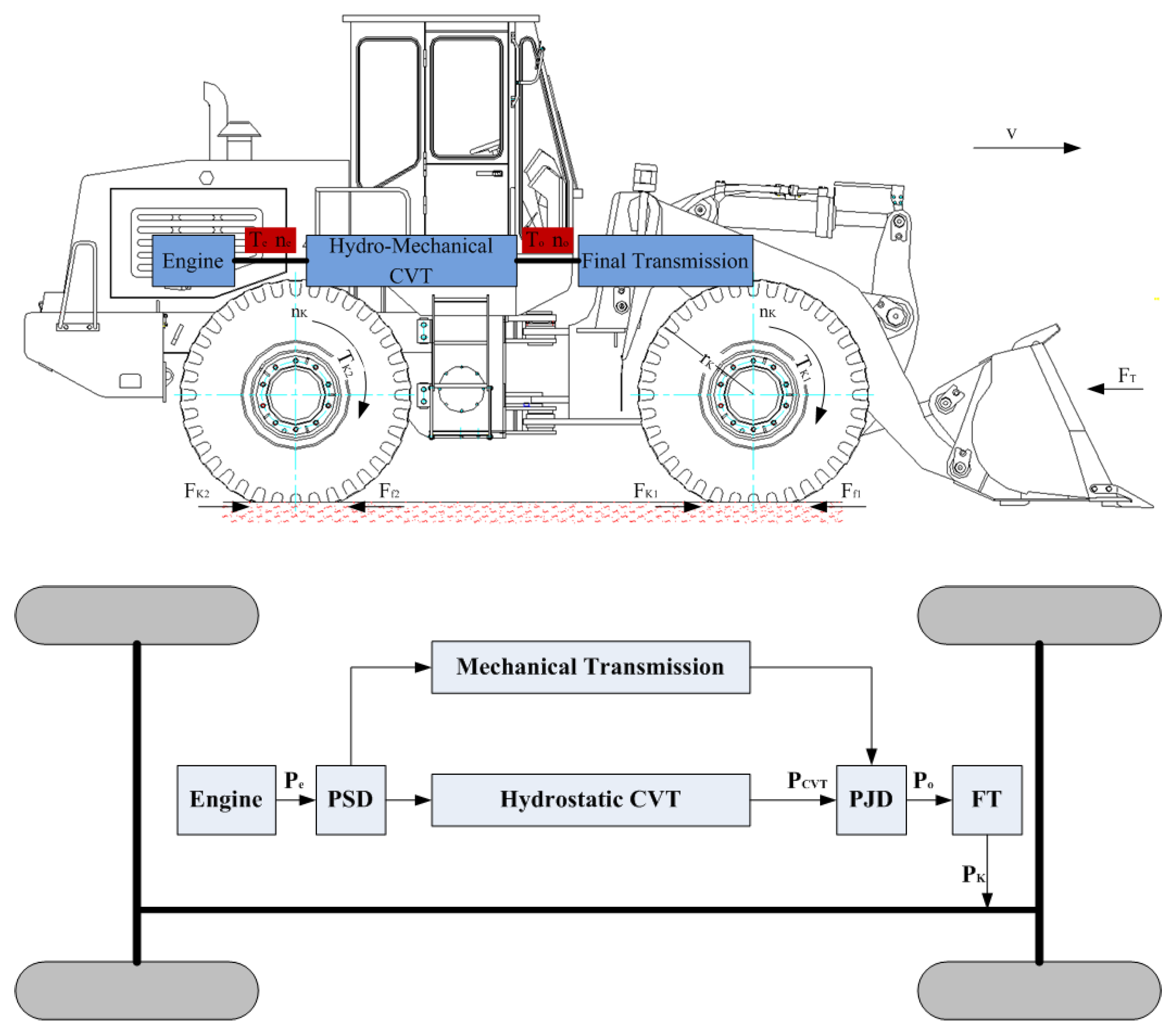
2. Analysis of the Wheel Loader Characteristics

2.1. Force Characteristics

The wheel loader is driven by the power of the engine, which is transmitted to the wheels through the transmission and driven by the driving force on the ground, as shown in Figure 2.
The driving force, F K , is used to overcome the driving resistance and driving traction of the loader. Driving resistance mainly refers to rolling resistance, F f , and air resistance, F ω . If the loader is driven uphill, it is necessary to overcome the ramp resistance, F i , caused by its own gravity; if the loader speeds up, it is also necessary to overcome the inertia force, F a . The driving force applied to the wheel loader, F K , can be calculated by the following equation:
F K = F T + F f + F ω + F i + F a
Under the working conditions, the loader is frequently accelerated and decelerated during the whole working cycle. Therefore, in view of the working conditions of the loader, the force characteristics under the accelerated state are mainly discussed. As shown in Figure 2, the loader is accelerating on the horizontal road. Because of the loading under the working conditions, the speed of the machine is relatively low, so the air resistance is neglected, then:
F K = F f + F a ;   F K = F K 1 + F K 2 ;   F f = F f 1 + F f 2 = f m t g ;   F a = m t a
Resultant torque of the wheels is shown in the following equation:
T K = ( F K 1 + F K 2 ) r K = ( f m t g + m t a ) r K
where T K is the driving torque of the wheel loader.

2.2. Velocity Characteristics

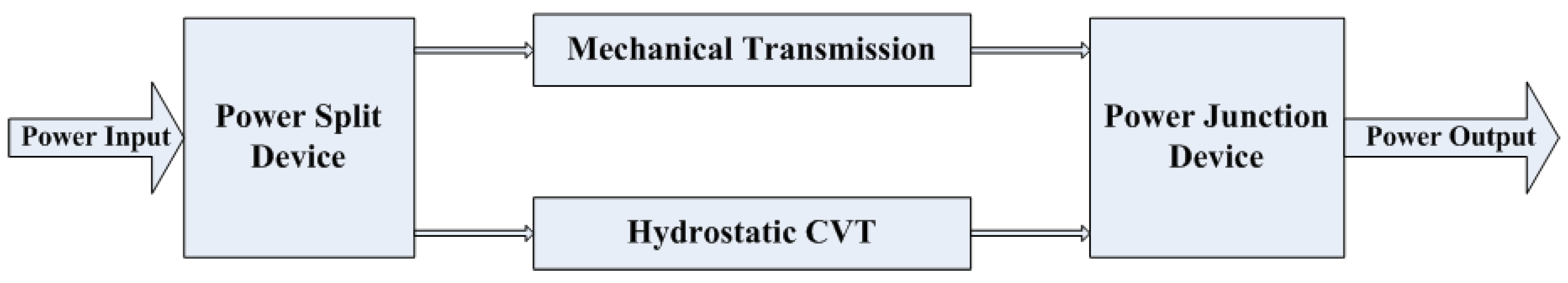
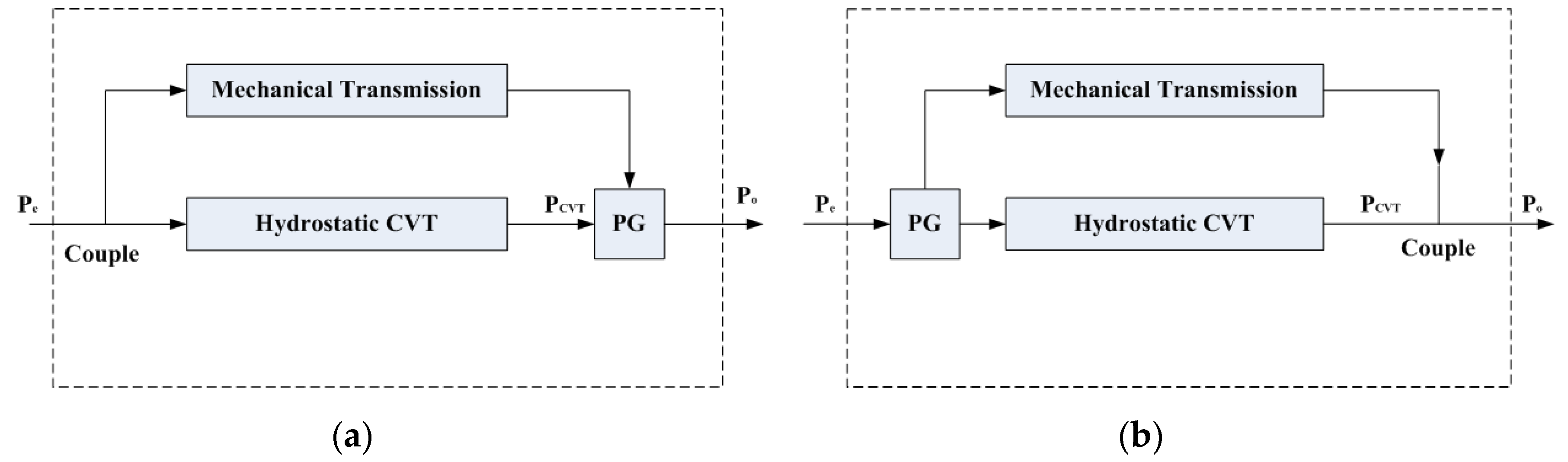
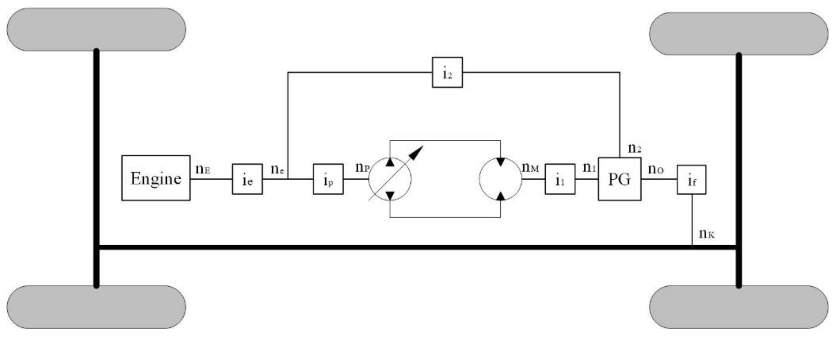
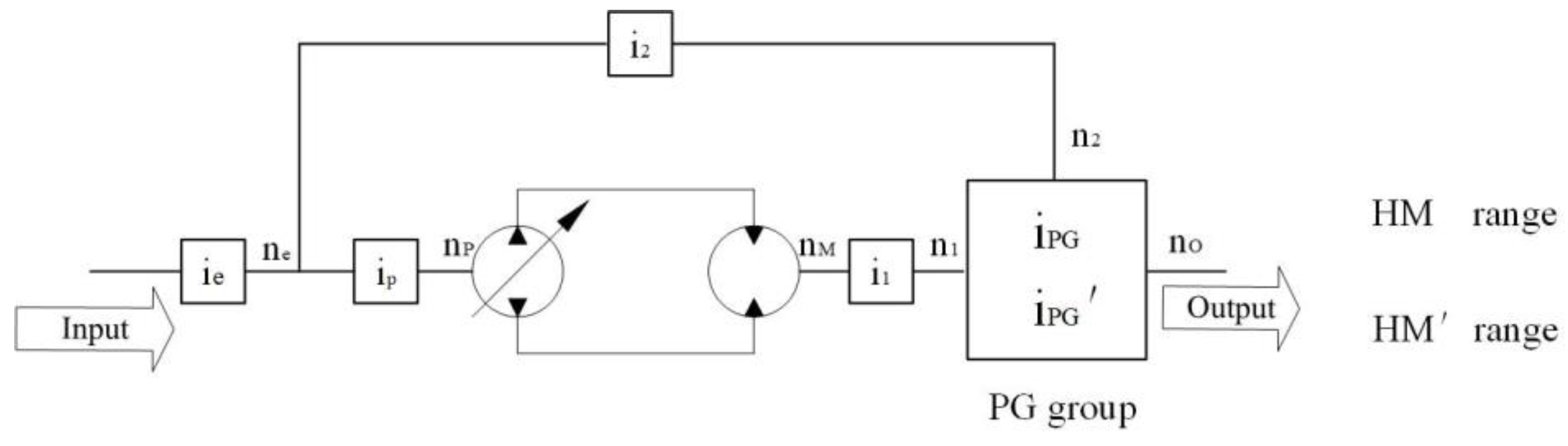
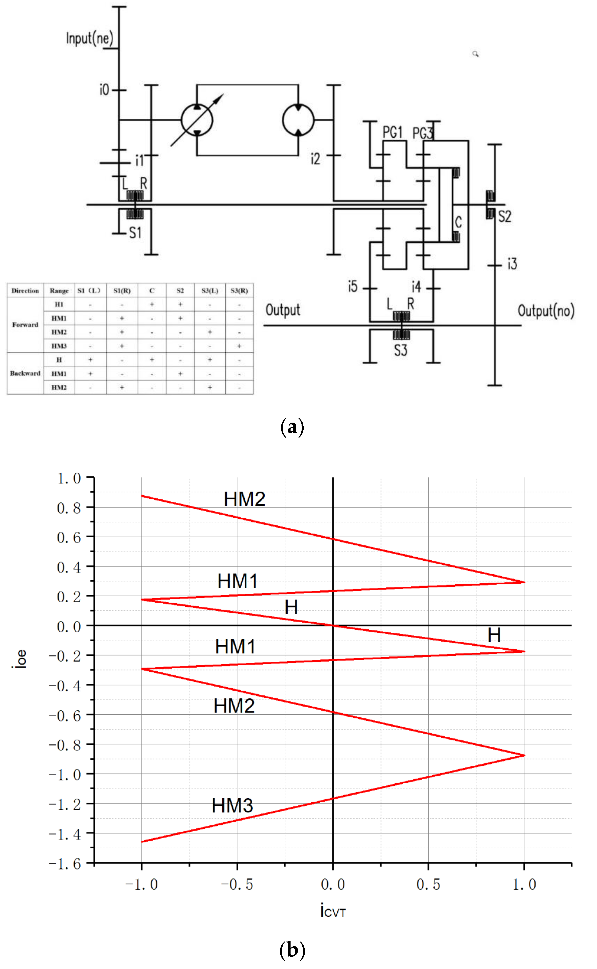
2.2.1. Types of HMCVT

HMCVT divides the power into two paths, one with a fixed transmission ratio (the mechanical path) and another which includes the hydrostatic CVT. Both rejoin in the output shaft [24]. The HMCVT relies on the Planetary Gear train (PG) to realize the function of power split or junction. There are two different types of the HMCVT, as shown in Figure 3. It is the input coupling type, as can be seen in Figure 3a, that has the PG as the power junction device (PJD), and the output coupling type, as can be seen in Figure 3b, that has the PG as the power-split device (PSD) [8,9].
When HMCVT speed range is required to be wide, in order to improve the efficiency, it is necessary to limit the speed range of hydrostatic CVT to reduce the proportion of hydrostatic CVT power flow. The mechanical transmission often shifts gears through the clutch or brake. Thus, when the transmission ratio of the hydrostatic CVT changes in different directions, the range of the transmission ratio of HMCVT will be enlarged, so that the proportion of hydrostatic CVT power flow in each speed range can be maintained as low as possible, realizing the efficient multi-range HMCVT with continuously varying transmission. Multi-range HMCVT mostly adopts this type of input coupling, because it can realize the high-efficiency operating point of all mechanical power flow. The Dana Rexroth (HVT) R2 and R3 adopt the three-range concept: The HVT has one hydrostatic drive range and two input coupling power-split ranges [4,5].
There are three working conditions in the basic components of the multi-range HMCVT:
  • H range, where the transmission has only hydrostatic power.
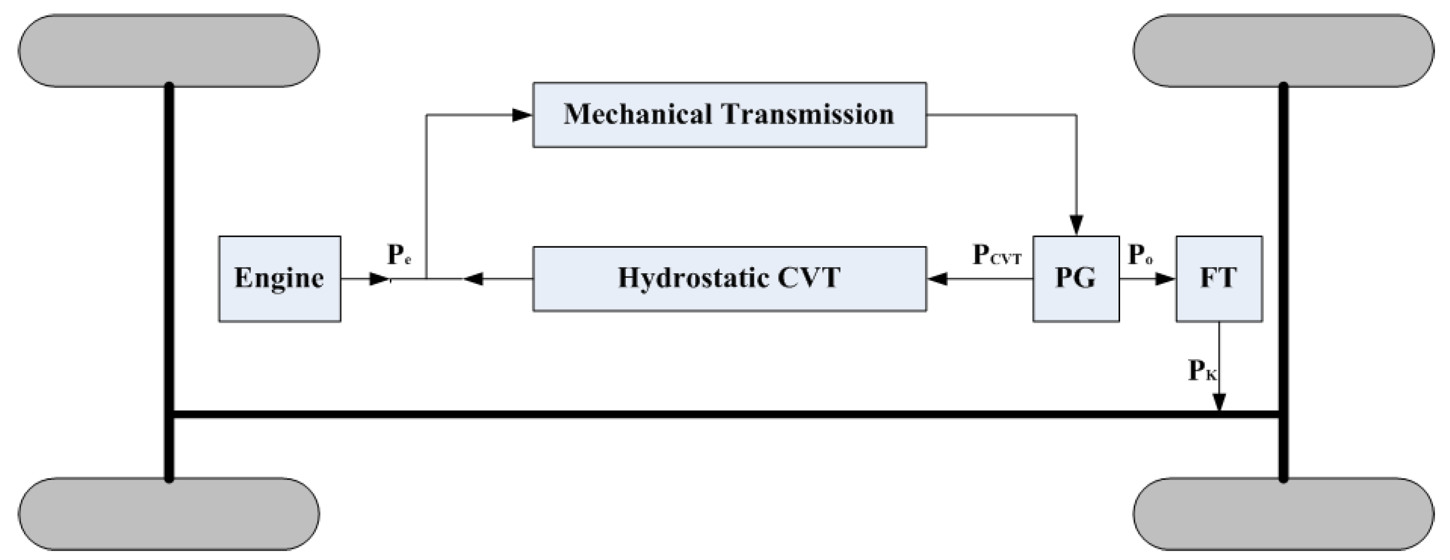
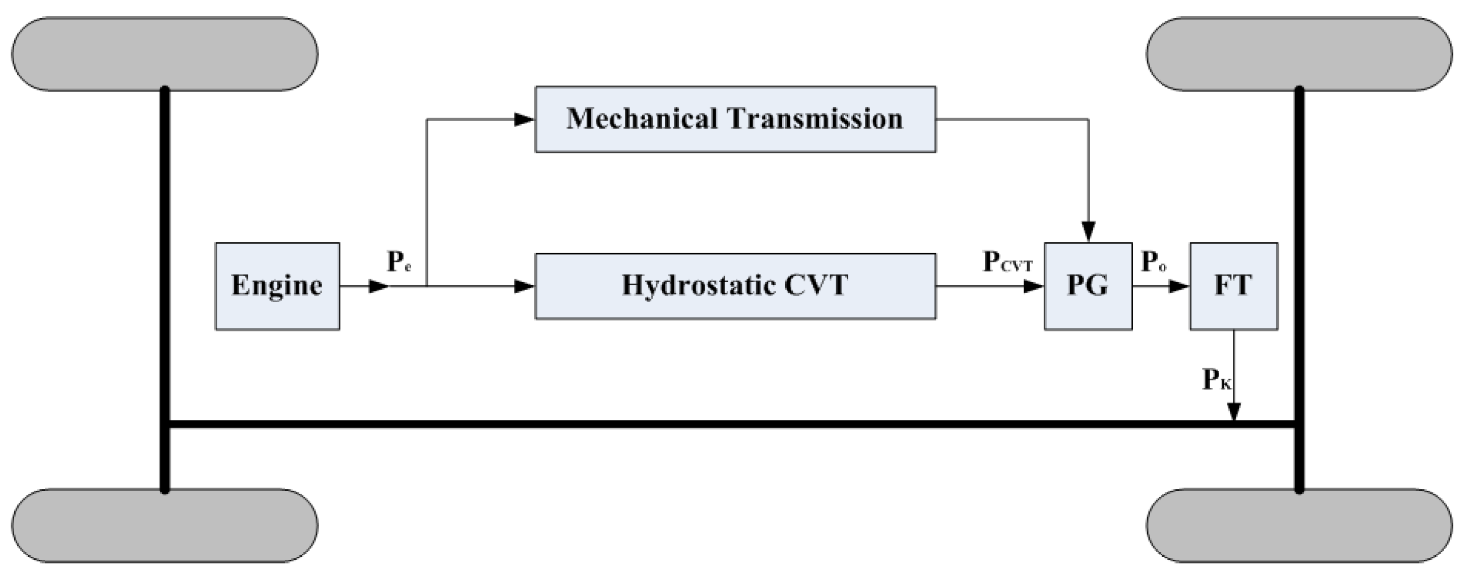
  • HM range, with forward transmission of the PG.
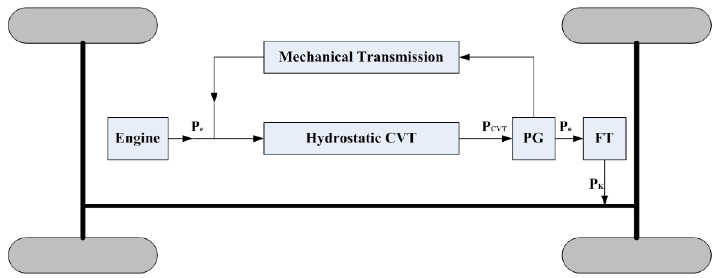
  • HM’ range, with reverse transmission of the PG.
There may be three working conditions in the whole process of the multi-range HMCVT, but the two-range transmission may also be composed of two of them. The H condition is only used in the starting working condition. In order to expand the range of the transmission ratio, HM and HM’ operation conditions may require one or several consecutive switching to achieve the required speed range.
In the input coupling type, the rotational speed direction of the variable displacement pump remains unchanged and it has small range of velocity variation. In the input coupling type, the variable displacement pump needs bidirectional rotation. Therefore, special variable displacement hydraulic pumps with reversible performance are required. Universal variable displacement pumps and motors can only be used for the input coupling type, so the input coupling type of the HMCVT is widely adopted, like Dana Rexroth (HVT) R2 and R3. Therefore, this paper focuses on in-depth study of the input coupling type.

2.2.2. Velocity Characteristics

The following equations can be derived from Figure 4:
i p = n e n P ,   i 1 = n M n 1 ,   i 2 = n e n 2 , i C V T = n M n P = V P V M
i P G = n o n 2 n 1 n 2 = T 1 T o
Then, the transmission ratio of the HMCVT becomes, by Equations (4) and (5),
i o e = n o n e = i C V T i P G i 2 i 1 i p i P G + i 1 i P i p i 1 i 2
and:
i C V T = i o e i p i 1 i 2 + i p i 1 i P G i 1 i p i P G i 2
i t = i f i e i o e = n E n K
where i p is the transmission ratio between shaft e and the pump, i 1 is the transmission ratio between the motor and shaft 1 of PG, i 2 is the transmission ratio between shaft e and shaft 2 of PG, i P G is the transmission ratio between output shaft and shaft 1, i C V T is the transmission ratio of hydrostatic CVT, i t is the transmission ratio of the whole transmission system, i e is the transmission ratio between engine and shaft e, i o e is the transmission ratio of HMCVT, i f is the transmission ratio between PG output shaft and the wheel, n E is engine speed, n e is shaft e speed, n P is pump shaft speed, n M is motor shaft speed, n 1 is shaft 1 speed of PG, n 2 is shaft 2 speed of PG, n o is output shaft speed of PG, n K is wheel speed, V P is pump displacement, and V M is motor displacement.
The range of transmission ratio, i o e , is:
α = i o e M i i o m = i C V T M i p G i 2 i 1 i p i P G + i 1 i p i C V T m i p G i 2 i 1 i p i P G + i 1 i p = β i C V T m i P G i 2 i 1 i p i P G + i 1 i p i C V T m i P G i 2 i 1 i p i P G + i 1 i p
and the range of i C V T is:
β = i C V T M i C V T m = i o e M i p i 1 i 2 + i p i 1 i P G i 1 i p i o e m i p i 1 i 2 + i p i 1 i P G i 1 i p = i o e M i 2 + i P G 1 i o e m i 2 + i P G 1
where i C V T M is the maximum value of i C V T , i C V T m is the minimum value of i C V T , i o e M is the value of i o e when i C V T = i C V T M , and i o e m is the value of i o e when i C V T = i C V T m .
The loader velocity is:
v = 2 π n K r K = 2 π n E r K i t

2.3. Power Characteristics

Assuming that the effect of efficiency is not taken into account, the following equations can be derived:
T 1 T o = i P G , T 1 T M = i 1 ,   T 1 T 2 = n 1 n o n 2 n o = i P G 1 i P G
The proportion of hydrostatic power in total power, ρ , can be obtained by Equations (6) and (12):
ρ = P C V T P K = P 1 P o = T 1 2 π n 1 T o 2 π n o = i P G i C V T i o e i p i 1
P K = F K v = F K 2 π n K r K = F K 2 π n E r K i t = F K 2 π n E i o e r K i f i e
By substituting Equation (6) into Equation (13), it becomes:
ρ = P C V T P K = i P G i 2 i C V T i C V T i P G i 2 i 1 i p i P G + i 1 i p
By substituting Equation (7) into Equation (13), it becomes:
ρ = P C V T P K = 1 ( i P G 1 ) i o e i 2
The following equation can be deduced by using the Equations (10), (14), and (16).
P C V T = [ 1 + β i e o m i e o M i o e ( 1 β ) ] F K 2 π n e i o e r K i f = [ 1 + β v m v M v ( 1 β ) ] F K v
The following conclusions can be obtained through Equation (17):
When v = β v m v M 1 β , ρ = 0 . The power of hydrostatic CVT is zero, HMCVT has only mechanical transmission to transmit power.
When v < β v m v M 1 β , ρ > 0 . Hydrostatic CVT occurs in backward power recirculation, as shown in the Figure 5.
When β v m v M v ( 1 β ) > 0 , ρ < 1 . Mechanical transmission occurs in backward power recirculation, as shown in Figure 6.
When v > β v m v M 1 β , β v m v M v ( 1 β ) > 0 , 1 < ρ < 0 . The power-split transmission has no recirculation, as shown in Figure 7.
Because of the low efficiency of hydraulic transmission, the optimum transmission mode is that the power-split transmission has no recirculation, as shown in Figure 7. The most undesirable transmission mode is that mechanical transmission occurs in backward power recirculation, as shown in Figure 6. When | ρ | > 1 , the efficiency of HMCVT is significantly reduced.

3. The Factors Influencing the Proportion of Hydrostatic Power

HMCVT adopts the fixed gear pair to achieve the power split. Input shaft of power is connected with the pump shaft through the fixed gear pair, then i p = 1 , as shown in Table 1.
When PG is used as PJD, the three components of sun gear, ring gear, and planetary gear connect hydrostatic CVT, mechanical transmission, and output shaft separately. There are 6 patterns, as shown in Table 1. k is the characteristic coefficient, and its range is 1.5–4.
The structure of the PSD and PJD is shown in Table 1, i p = 1 . Then:
i o e = n o n e = i C V T i P G i 2 i 1 i P G + i 1 i 1 i 2
and
T o = i 1 i P G T M
Derivation of Equation (18):
i o e i C V T = i P G i 1
Considering the compactness of gear transmission structure, the range of the value i 1 is −1 to −3. In Schemes 1, 2, 4, and 6, i P G > 0 , then, i P G i 1 < 0 . Therefore, the transmission ratio, i o e , is a monotonic decreasing function of i C V T . In Schemes 3 and 5, i P G < 0 , then, i P G i 1 > 0 . The transmission ratio, i o e , is a monotonic increasing function of i C V T .
The variable speed range of the single-range HMCVT cannot meet that of the wheel loader. Multi-range HMCVT is adopted and requires two planetary gear trains to achieve shifting, as shown in Figure 8.
According to i P G > 0 or i P G < 0 , the transmission ratio, i o e , is a monotonic decreasing or increasing function of i C V T . When i P G > 0 , it is HM range with forward transmission of the PG ( i P G ); when i P G < 0 , it is HM’ range with reverse transmission of the PG ( i P G ). Therefore, there are four PG matching patterns to realize the range shifting between hydro-mechanical ranges, as shown in Table 2.
When the vehicle starts, the transmission system is in H condition and ρ = 1 . Then:
i o e = n o n e = i C V T i 1
The transmission ratio, i o e , is a monotonic decreasing function of i C V T . To realize the same speed shift connection between H range and hydro-mechanical range, the Scheme 3 or Scheme 5 of HM’ range can connect with H range. Hence, it needs to make i 1 = i 2 i C V T M , and for the Schemes 1, 2, 4, and 6 of the HM range to connect with the HM’ range, it needs to make i P G = i P G to achieve equal difference between hydro-mechanical ranges.
Next, the rules of the transmission ratio, i o e , and hydrostatic CVT power proportion, ρ , under these conditions, as shown in Table 1, are studied. Let i 1 = i 2 i C V T M = i , Equation (18) becomes:
i o e = n o n e = i C V T i P G i C V T M i P G + i C V T M i
and
i o e M = i C V T M i
The following equations can be concluded by using Equations (9), (10) and (22):
α = β i P G β i P G + β
ρ = i P G i C V T i P G i C V T i C V T M i P G + i C V T M
when i C V T = i C V T M , i C V T = i C V T m , it can be concluded:
ρ M = i P G ;   ρ m = i P G i P G β i P G + β = α β i P G
Suppose that i C V T changes symmetrically in two directions, i.e., β = 1 , i C V T M = 1 , then:
ρ = i P G i C V T i P G i C V T i P G + 1
α = 1 2 i P G 1
ρ m = i P G 2 i P G 1 = α i P G
From the Equations (26)–(29), ρ M , ρ m , and α are independent of i C V T M , and only related to i P G .
When i C V T changes symmetrically in two directions, i.e., β = 1 , the following conclusions can be drawn:
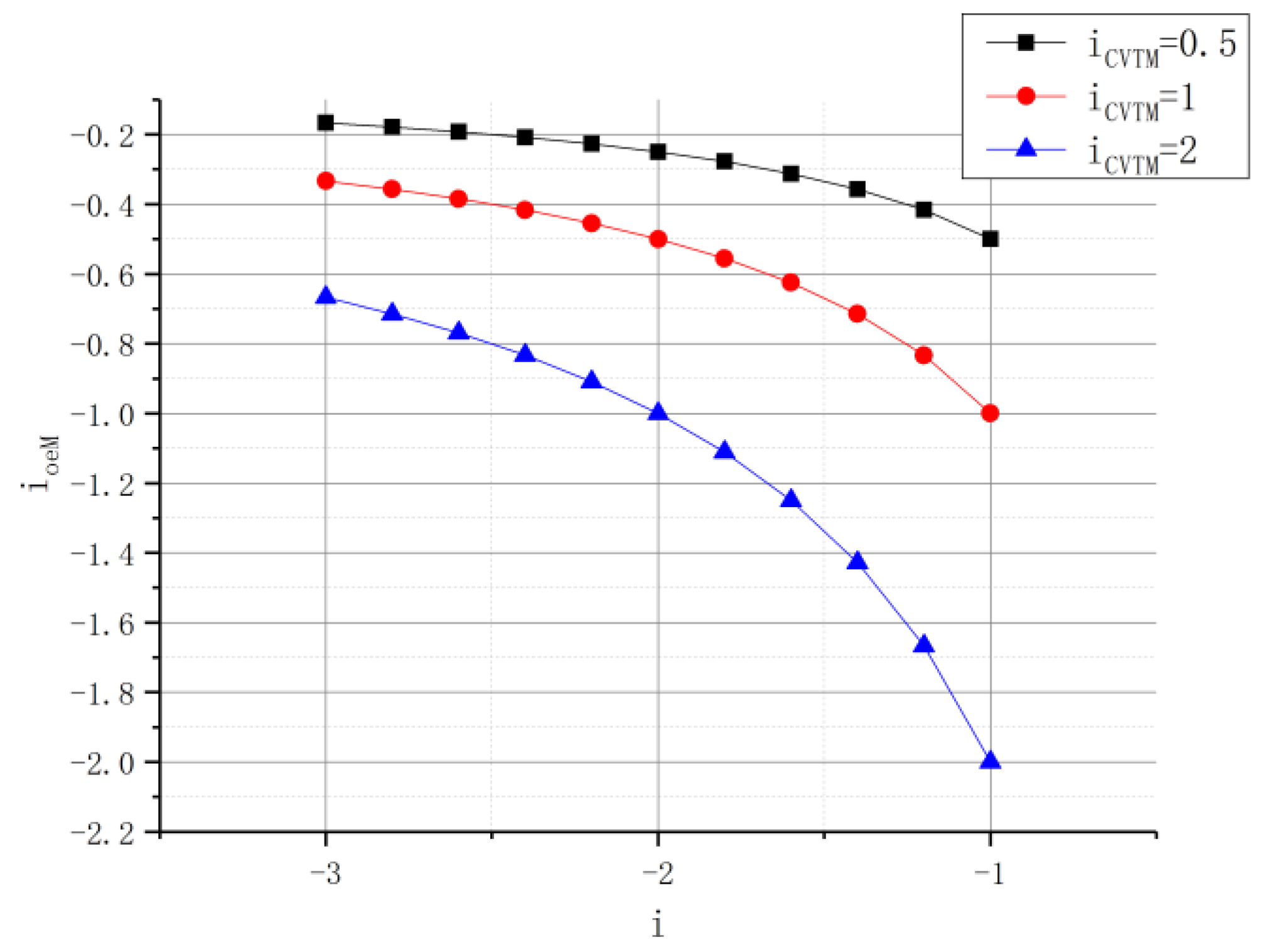
  • To realize the same speed shift connection between the H range and hydro-mechanical range, as you can see from Equation (23) and Figure 9, when i p = 1 , | i o e M | increases with the increase of | i C V T M | and decreases with the increase of | i 1 | .
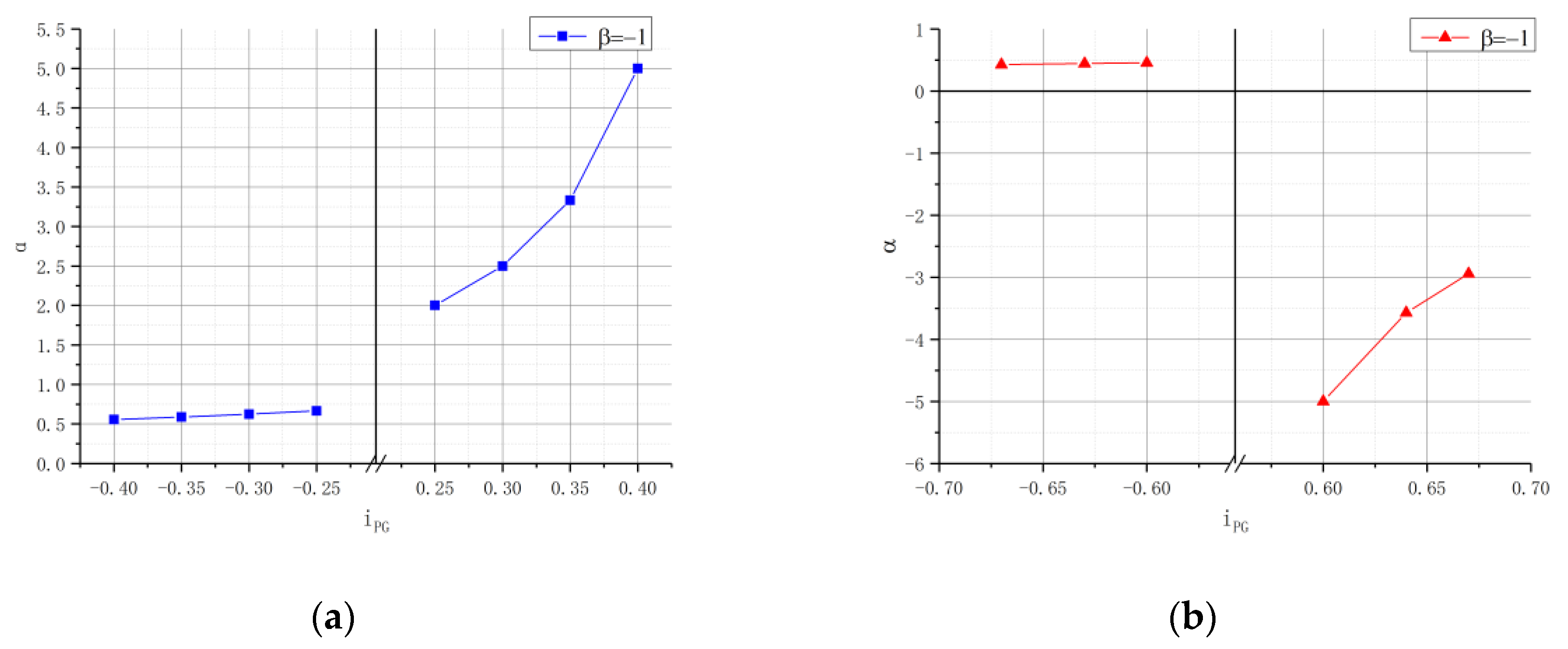
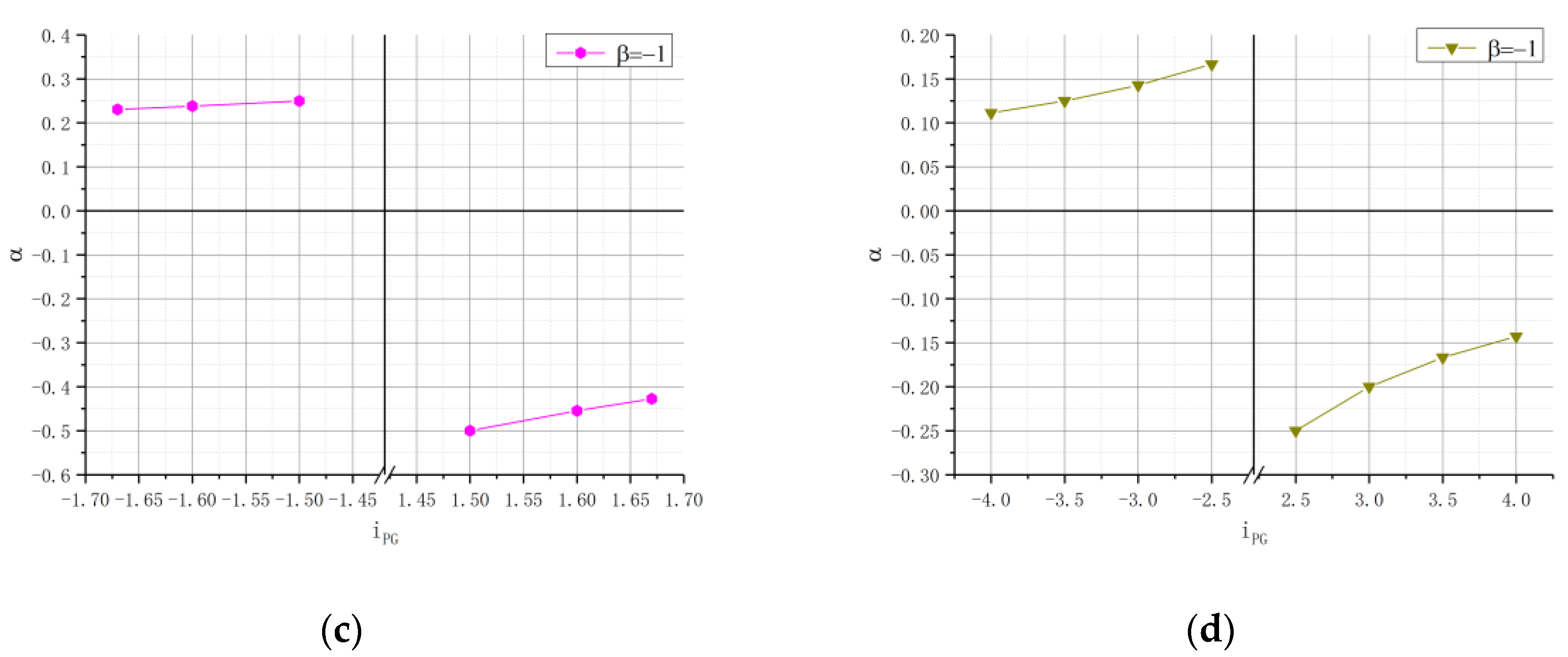
  • As can be seen from Equation (19), under certain conditions of T M , | T o | increases with the increase of | i 1 | and decreases with the increase of | i P G | . So, matching patterns a and b have better torque characteristics than matching patterns c and d in Table 2.
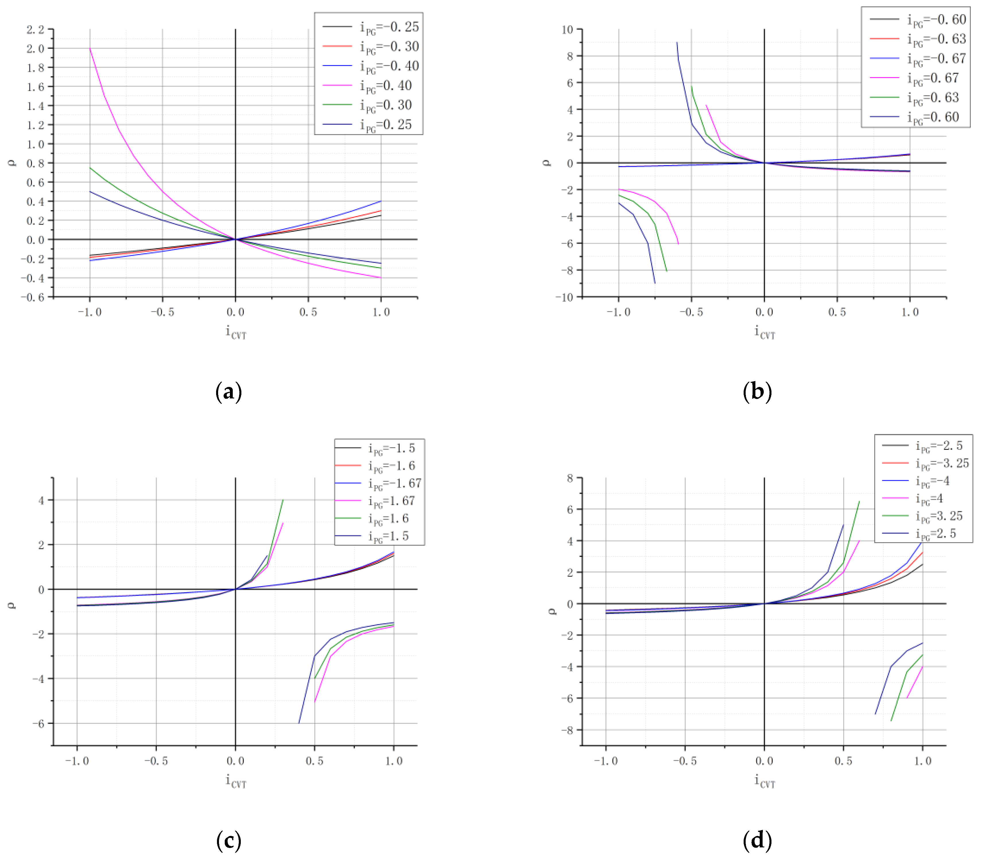
  • From Equation (28) and Figure 10, the range of transmission ratio, α , increases with the increase of i P G , and Schemes 2, 4, and 6 exist as i o e = 0 because of α < 0 .
  • From the Equations (26), (27), (29), and Figure 11, ρ M and ρ m are independent of i C V T M , and only related to i P G . Schemes 2, 4, and 6 exist as the work condition with the lowest transmission efficiency because mechanical transmission occurs in backward power recirculation, i.e., ρ < 1 , as shown in Figure 6. The transmission efficiency of matching patterns b, c, and d are lower than matching pattern a because | ρ M | > 0.6 and mechanical transmission occurs even in backward power recirculation, as shown in Figure 6. Therefore, the efficiency of HMCVT is significantly reduced.
Therefore, the best matching pattern is Pattern a. Assume that β ranges from −1 to −2, then the variation of α , ρ M , and ρ m are shown in Figure 12 and Figure 13.
From Figure 11 and Equation (24), α is related to i P G and β . In Scheme 1, α increases with the increase of i P G and β , In Scheme 3, α increases with the increase of i P G , and decreases with the increase of β .
From Equations (25), (26), and Figure 13, the factor influencing on ρ M is i P G , and factors influencing on ρ m are i P G and β . ρ M decreases with the increase of i P G , as shown at the bottom of Scheme 1 and the top of Scheme 3, and | ρ m | increases with the increase of β and | i P G | , as shown at the top of Scheme 1 and the bottom of Scheme 3.

4. The Efficiency Analysis of the Matching Pattern A

Theoretical Calculation

Through the above analysis, the best matching pattern is established. In this section, the efficiency of pattern a is analyzed concretely. Two schemes of pattern a have two power transmitting modes, as shown in the Figure 14. The nodal power method can be used to establish their efficiency formulas.
In the Mode I in Figure 14a, the power transmitting has no recirculation. Both the hydrostatic CVT power, P C V T , and the mechanical transmission power, P M T , are forward transferring, i.e., 1 < ρ < 0 . The efficiency formula of Mode I is:
η I = | P C V T η C V T η p η 1 η 1 o 2 + P M T η 2 η 2 o 1 P e |
The following formula can be concluded by using Equations (15) and (30):
η I = | i C V T i P G i 2 η C V T η p η 1 η 1 o 2 + i 1 i p ( 1 i P G ) η 2 η 2 o 1 i C V T i P G i 2 i 1 i p i P G + i 1 i p |
In the Mode Ⅱ in Figure 14b, the power transmitting has recirculation of hydrostatic CVT power. The mechanical transmission power, P M T , is forward transferring, i.e., ρ > 0 . The efficiency formula of Mode Ⅱ is:
η II = | P o | P e = | η 2 η 2 o 1 i C V T i P G i 2 i 1 i p i P G + i 1 i p [ i 1 i p ( 1 i P G ) + i C V T i P G i 2 η C V T η p η 1 η 21 o ] |
where η I is the efficiency of Mode Ⅰ, η II is the efficiency of Mode Ⅱ, η C V T is hydrostatic CVT efficiency, η 1 is the efficiency of gear set 1, η 2 is the efficiency of gear set 2, η p is the efficiency of gear set p, η 21 o is the efficiency between shaft 2 and shaft 1 of PG, η 1 o 2 is the efficiency between shaft 1 and output shaft of PG, and η 2 o 1 is the efficiency between shaft 2 and output shaft of PG.
As shown in Figure 14, there are efficiency problems in Variable Displacement Hydraulic Pump (VP), Fixed Displacement Hydraulic Motor (FM), the control valve group, and the connecting pipes, which affect the efficiency of hydrostatic CVT. Therefore, the volumetric efficiency of hydrostatic CVT is a dynamic changing process. Without regard to the efficiency loss of connecting pipes and the control valve group, the efficiency calculation is simplified as follows:
η C V T v = η P v η M v ;   η C V T m = η P m η M m ;   η C V T = η P t η M t = η P v η P m η M m η M v
where η C V T v is volumetric efficiency of hydrostatic CVT, η C V T m is mechanical efficiency of hydrostatic CVT, η P v is volumetric efficiency of VP, η P m is mechanical efficiency of VP, η P t is total efficiency of VP, η M v is volumetric efficiency of FM, η M m is mechanical efficiency of FM, and η M t is total efficiency of FM.
The HMCVT efficiency of Schemes 1 and 3 is as follows:
As seen Schemes 1 and 3 in Table 1, i p = 1 . Let i C V T M = 1 , i C V T m = 1 , then i 1 = i 2 = i , η p = 1 , η 1 = η 2 = 0.97 . In Scheme 1, when 0 i C V T 1 , 1 < ρ < 0 , power transmitting mode is Mode I. When 1 i C V T 0 , ρ > 0 , power transmitting mode is Mode II. The change rule of Scheme 3 is contrary to Scheme 1. The efficiency of the mechanical gear transmission is usually calculated by meshing power method. The efficiency of outer gearing is 0.97, and the efficiency of inner gearing is 0.98. Then, the HMCVT efficiency of Scheme 1, η s 1 , and Scheme 3, η s 3 , in Table 1 are:
η s 1 = { | 0.97 0.0485 i P G i C V T i P G i P G + 1 [ ( 1 i P G ) + i C V T i P G 0.9215 η C V T ] | 1 i C V T < 0 | i C V T i P G η C V T ( 0.0485 i P G + 0.9215 ) + ( 1 i P G ) ( 0.97 0.0485 i P G ) i C V T i P G i P G + 1 | 0 i C V T 1
and
η s 3 = { | 0.9215 i C V T i P G η C V T ( 0.95 i P G ) + 0.9215 ( 1 i P G ) 2 ( i C V T i P G i P G + 1 ) ( 0.95 i P G ) | 1 i C V T < 0 | 0.9215 ( 1 i P G ) 2 η C V T + i C V T i P G ( 1 0.95 i P G ) ( i C V T i P G i P G + 1 ) ( 0.95 i P G ) η C V T | 0 i C V T 1
Assuming that the efficiency of hydrostatic CVT is 0.8, then the efficiency curves of Schemes 1 and 3 in Table 1 are shown in Figure 15.
From (a) in Figure 11 and Figure 15, it can be concluded that η s 1 and η s 3 are related to i P G and i C V T . η s 1 and η s 3 increase with the decrease of | i C V T | and | i P G | , i.e., increases with the decrease of | ρ | . The efficiency of Mode I is higher than Mode II. The efficiency value of HMCVT is between that of hydrostatic CVT and mechanical transmission.

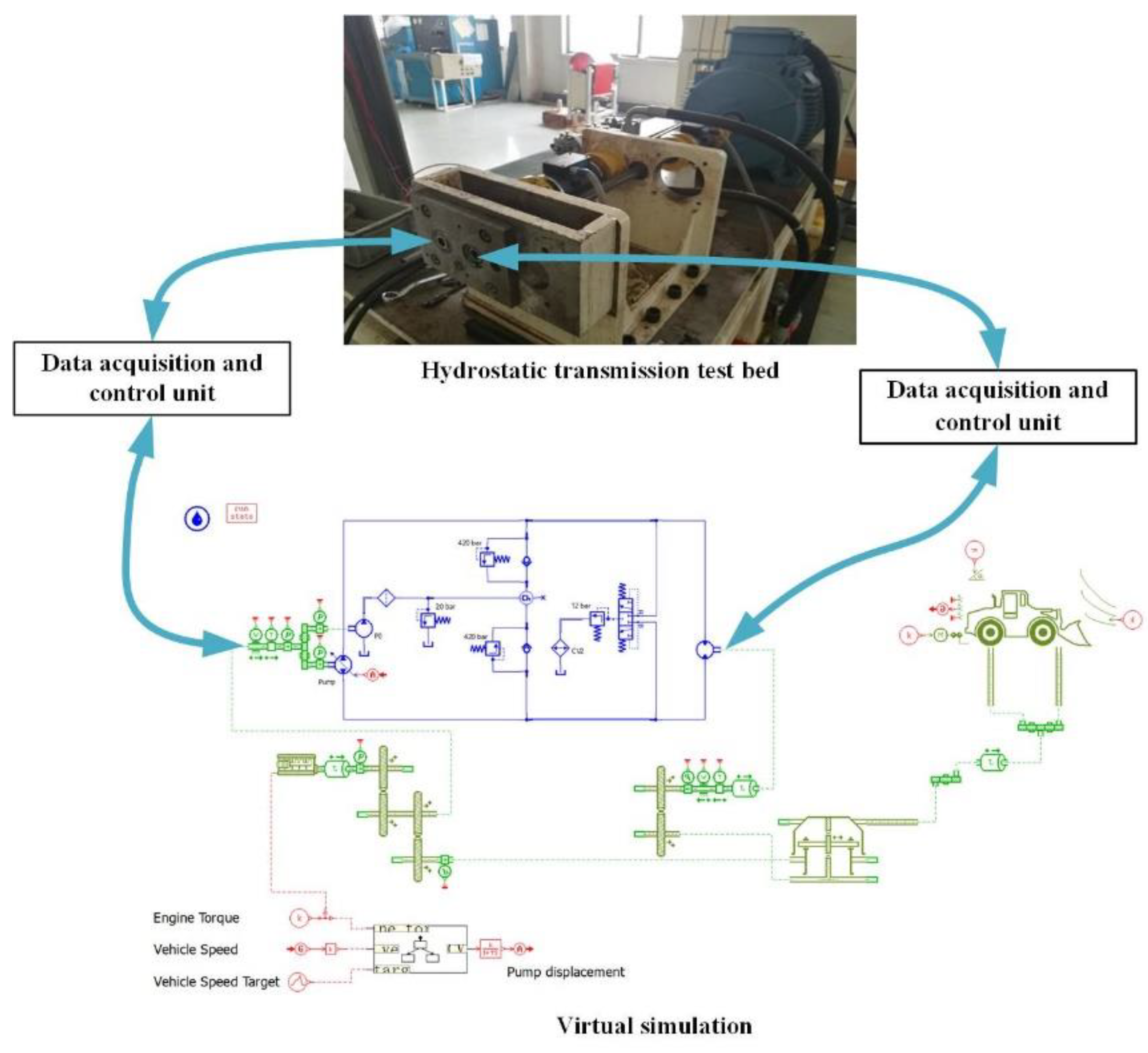
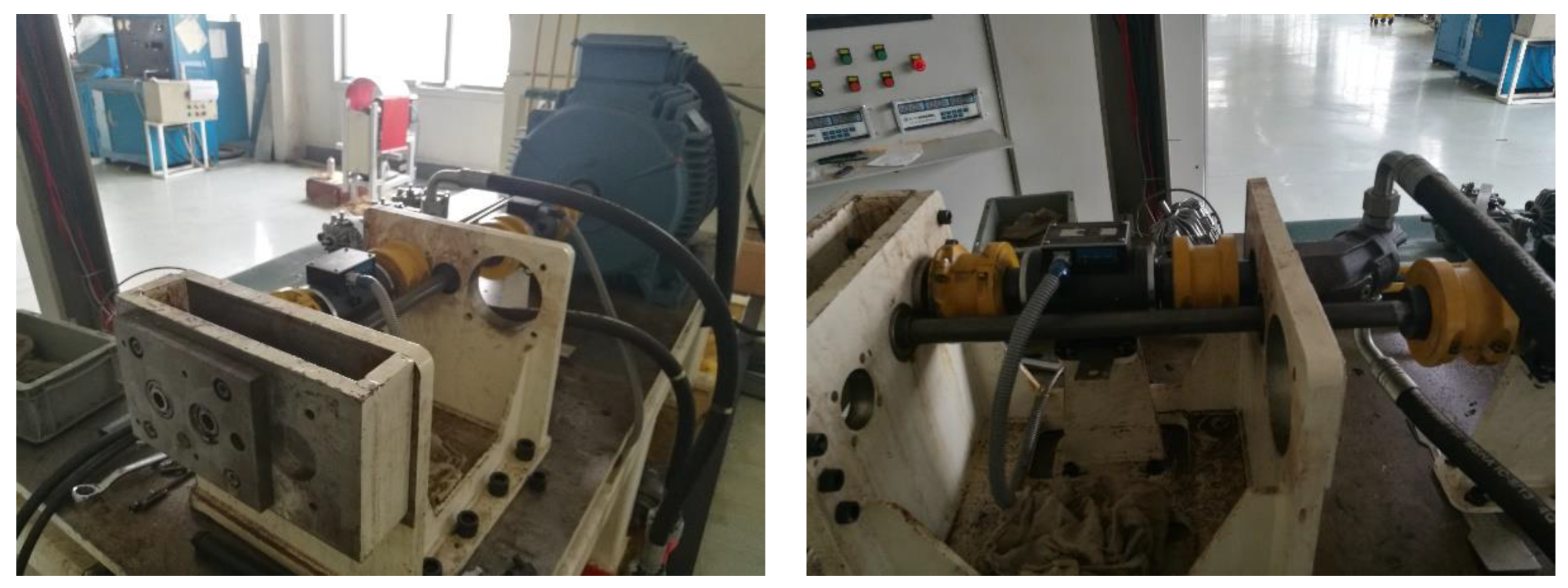
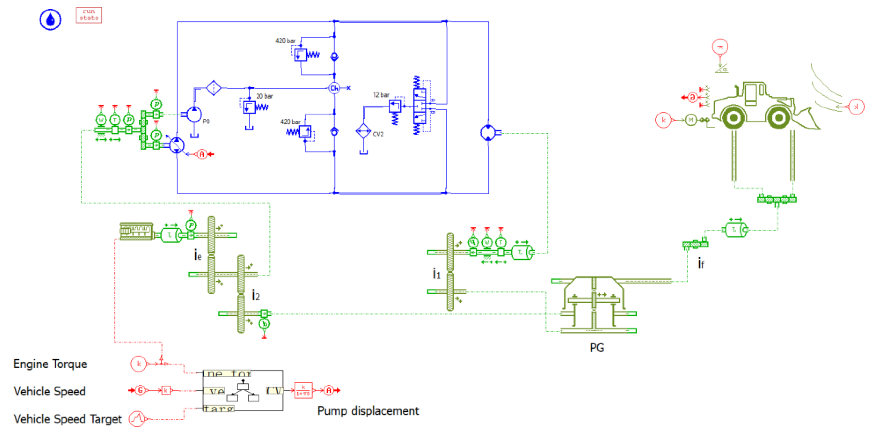
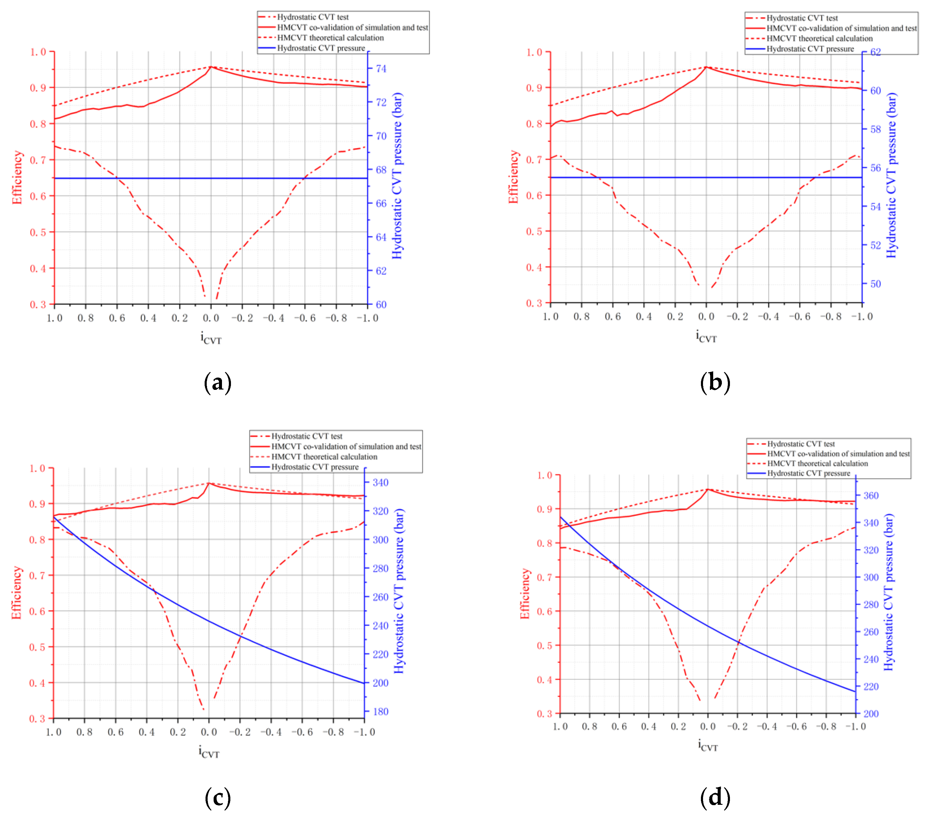
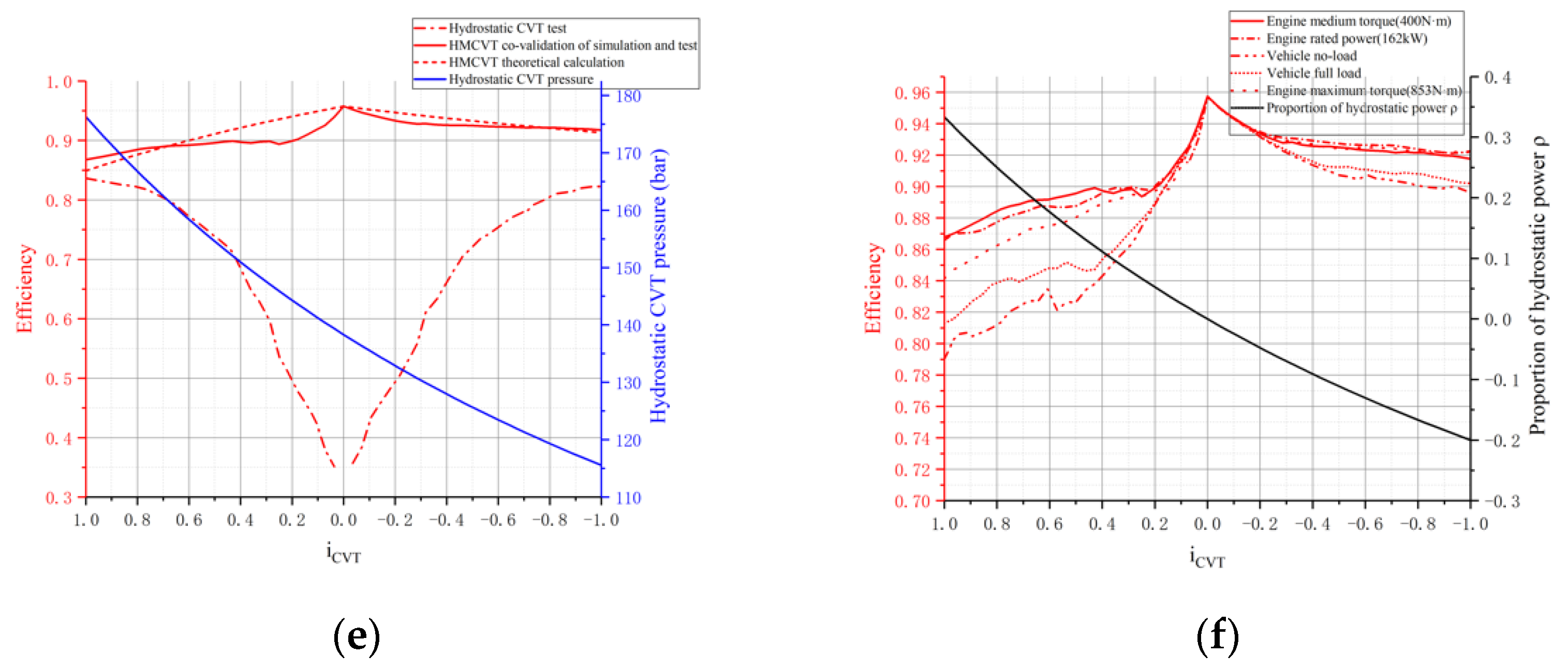
5. Co-Validation of Simulation and Test

5.1. The Method of Co-Validation

Compared with the mechanical transmission, the efficiency of the hydraulic transmission is relatively low, and the efficiency constantly changes during variable speed. To more accurately analyze the efficiency of the transmission system, this paper adopts the method of co-validation of the simulation and test, as shown in Figure 16.
It is the method that combines the test of the hydrostatic transmission with the simulation of the HMCVT by the data acquisition and control unit. It mainly realizes the exchange of simulation and test data through the data acquisition unit and controls the hydrostatic transmission test bed through the control unit. Torque and speed of VP and FM are obtained through simulation analysis, and the loading system is controlled by the control unit according to the simulation date. Torque and speed of VP and FM are measured through sensors and their dates are obtained through the acquisition unit; eventually, the actual efficiency of the hydrostatic transmission can be calculated. Then, the efficiency data are input to the simulation model to achieve more accurate simulation. Therefore, it can realize validation in the early stage of HMCVT design to avoid the irrationality of the structure after the developed prototype.
The rotational speed and pressure of VP and FM are constantly changing, therefore hydrostatic CVT efficiency, η C V T , is also constantly changing. Its efficiency characteristic is obtained by testing on the test bed. The physical diagram of the hydrostatic transmission test bed is shown in Figure 17.
The power source of the test bed is driven by a motor, and the hydraulic loading system is used to load the output shaft of the hydrostatic transmission. Its input and output shafts are equipped with speed and torque sensors.

5.2. The Application of Test and Validation

In order to validate the correctness of the above analysis, in this paper, an example is given to verify the validity of the method. Take a wheel loader as an example, the parameters are shown in Table 3.
According to the parameters of a wheel loader, the structural scheme of the multi-range HMCVT is designed and the transmission ratio, i o e , is analyzed, as shown in Figure 18.
Where i0, i1, i2, i3, i4, and i5 are the transmission ratio of gear sets, S1, S2, and S3 are synchronizers, C is clutch, PG1 is the Scheme 1 of PG, and PG3 is the Scheme 3 of PG. The table is the engagement state of synchronizers or clutch, in which positive is coupled and negative is uncoupled.
It can be seen from Figure 18 that the forward direction of a multi-range HMCVT consists of a pure hydrostatic range (H range) and three hydrostatic and mechanical transmission ranges (HM1, HM2, and HM3 range). The backward direction consists of a pure hydrostatic range (H range) and two hydrostatic and mechanical transmission ranges (HM1 and HM2 range). The performance of each range can be tested and analyzed in the same method of co-validation; therefore, this paper takes one range to carry out co-validation.
The HM1 range is a commonly used range in the working process of the loader and takes Scheme 3 in Table 1 as PJD. During the HM1 range, the load of the wheel loader has a large range of changes, and the largest traction force also occurs in this range. Therefore, this paper takes the HM1 range as the research object to analyze under five typical working conditions, as shown in Table 4.
Under the working condition of engine maximum torque, the engine speed is 1500 rpm and the vehicle speed is 1.125~1.857 m/s during the HM1 range; under the others, the engine speed is 2000 rpm and the vehicle speed is 1.5~2.5 m/s. The HM1 range transmission system simulation model is built by using AMESim software, and the simulation model is shown in Figure 19.
Through the co-validation method of simulation and test, the analysis results are shown in Figure 18.
As can be seen from Figure 20a–e, the efficiency of the hydrostatic CVT is significantly reduced with the reduction of i C V T , and reaches the lowest value when approaching zero. At this time, the inclination of the VP swash plate is near zero, which results in the FM output speed approaching zero. Therefore, the mechanical efficiency is greatly reduced, and causes the efficiency of hydrostatic CVT to reach the lowest. However, the proportion of hydrostatic power in total power, ρ, is also close to zero, hence it has little effect on the efficiency of HMCVT, and the highest efficiency of HMCVT is at i C V T = 0 .
It can be seen from Figure 20a,b that the pressure in the CVT system is constant, because the vehicle is running at constant torque under the working conditions of no-load and full load. Therefore, the efficiency of hydrostatic CVT basically changes symmetrically on both sides of i C V T = 0 . However, as shown in Figure 20c–e, the vehicle is running at constant power, and the output torque is constantly changing, hence the pressure decreases with the decrease of i C V T . Therefore, the efficiency of hydrostatic CVT changes differently on both sides of i C V T = 0 . When the pressure is 200~240 bar in Figure 20c, and 220~255 bar in Figure 20d, the efficiency of hydrostatic CVT on the right of i C V T = 0 is higher than the left at the same value of | i C V T | . When the pressure is 150~180 bar in Figure 20e, its efficiency on the right of i C V T = 0 is lower than the left. As shown in Figure 20c, when the pressure is 200 bar and the VP displacement reaches the maximum displacement, the efficiency of hydrostatic CVT is the highest, which is 0.849.
As shown in Figure 20f, when 0 > i C V T > 1 , 0.2 < ρ < 0 , and the power transmitting has no recirculation, when 0 < i C V T < 1 , 0 < ρ < 0.33 , and the power transmitting has recirculation of hydrostatic CVT power. Therefore, the efficiency of HMCVT on the right of i C V T = 0 is lower than on the left. Under the working conditions of engine medium torque and engine rated power, the efficiency of HMCVT is higher than others, in which the minimum efficiency is above 0.86. Under the working condition of vehicle no-load, the efficiency of HMCVT is the lowest, but the minimum efficiency is still close to 0.80.

6. Conclusions

To better study the characteristics of HMCVT applied to the wheel loader, this paper established the characteristic equations of input coupling type of HMCVT based on the wheel loader characteristics and analyzed power flow transmission modes of HMCVT. Then, this paper studied and analyzed factors influencing the proportion of hydrostatic power, which was mainly from the connection of working conditions and the structure of the planetary arrangement. The results show that factors influencing the proportion of hydrostatic power in total power ( ρ ) are transmission ratio between the output shaft and shaft 1 ( i P G ), the range of hydrostatic CVT transmission ratio ( β ), not related to transmission ratio between motor and shaft 1 of PG ( i 1 ), transmission ratio between shaft e and shaft 2 of PG ( i 2 ), and transmission ratio between shaft e and the pump ( i p ).
The best matching pattern was established through comparison analysis. This paper established the efficiency equations of Schemes 1 and 3, and the efficiency of pattern (a) was analyzed concretely. The analysis results showed that HMCVT efficiency of Schemes 1 and 3 was related to the transmission ratio between the output shaft and shaft 1 ( i P G ), and the hydrostatic CVT transmission ratio ( i C V T ).
In the early design process, this paper presented a method of co-validation of the simulation and test to make the results of efficiency more accurate. Taking a specific wheel loader as an example, this method can be applied to analyze the efficiency under different working conditions. The results show that: When the pressure is 50% of the maximum pressure, and the pump displacement reaches the maximum displacement, the efficiency of hydrostatic CVT reaches the highest, and the efficiency of HMCVT is also the highest, which is more accurate than the theoretical calculation results. It provides an important guiding role and validation in the early design of HMCVT to avoid the irrationality of the structure after the prototype manufacturing. Eventually, the design cost and cycle are saved.

Author Contributions

L.W. and H.D. contributed the major part of this work: literature review, analysis of the wheel loader characteristics and influencing factors of the proportion of hydrostatic power, efficiency calculation and simulation and manuscript drafting and revising. Q.Z. provided some advices on the HMCVT and modeling, and also checks the theoretical derivation and figures. Z.S. and M.T. provided the test data and data collection. All authors have read and agreed to the published version of the manuscript.

Funding

This research was funded by Supported by Special funds for Climbing Project of Taishan Scholars, National Natural Science Foundation of China (Grant No. 51674155), Innovative Team Development Project of Ministry of Education (Grant No. IRT_16R45), and Shandong Natural Science Foundation (Grant No. ZR201807080343).

Conflicts of Interest

The authors declare no conflict of interest.

Abbreviations

The following abbreviations are used in this manuscript:
HMCVTHydro-Mechanical Continuously Variable Transmission
CVTContinuously Variable Transmission
PSDPower-Split Device
PJDPower Junction Device
FTFinal Transmission
PGPlanetary Gear train
VPVariable Displacement Hydraulic Pump
FMFixed Displacement Hydraulic Motor
F K Driving force of the wheel loader
F f Rolling resistance of the wheel loader
F ω Air resistance of the wheel loader
F i Ramp resistance of the wheel loader
F a Inertia force of the wheel loader
m t Total weight of the wheel loader
i t Transmission ratio of the whole transmission system.
i e The transmission ratio between engine and shaft e
i p The transmission ratio between shaft e and pump
i 1 Transmission ratio between motor and shaft 1 of PG
i 2 Transmission ratio between shaft e and shaft 2 of PG
i P G Transmission ratio between output shaft and shaft 1
i C V T Transmission ratio of Hydrostatic CVT
i o e Transmission ratio of HMCVT
i f Transmission ratio between PG output shaft and the wheel
n E Engine speed
n e Shaft e speed
n P Pump shaft speed
n M Motor shaft speed
n 1 Shaft 1 speed of PG
n 2 Shaft 2 speed of PG
n o Output shaft speed of PG
n K Wheel speed
V P Pump displacement
V M Motor displacement
T 1 Shaft 1 torque of PG
T 2 Shaft 2 torque of PG
T o Output shaft torque of PG
T M Motor shaft torque
T K Driving torque of wheel loader
T E Engine torque
α The range of transmission ratio, i o e
β The range of i C V T
v Wheel loader velocity
r K Radius of wheel
ρ Proportion of hydrostatic power in total power
P o Output power of HMCVT
P K Driving power
P C V T Hydrostatic CVT power
P M T Mechanical Transmission power
k PG characteristic coefficient
η I Efficiency of mode Ⅰ
η II Efficiency of mode Ⅱ
η C V T v Volumetric efficiency of Hydrostatic CVT
η C V T m Mechanical efficiency of Hydrostatic CVT
η P v Volumetric efficiency of VP
η P m Mechanical efficiency of VP
η P t Total efficiency of VP
η M v Volumetric efficiency of FM
η M m Mechanical efficiency of FM
η M t Total efficiency of FM
η C V T Hydrostatic CVT efficiency
η 1 Efficiency of gear set 1
η 2 Efficiency of gear set 2
η p Efficiency of gear set p
η 21 o Efficiency between shaft 2 and shaft 1 of PG
η 1 o 2 Efficiency between shaft 1 and output shaft of PG
η 2 o 1 Efficiency between shaft 2 and output shaft of PG
η s 1 HMCVT efficiency of scheme 1
η s 3 HMCVT efficiency of scheme 3

References

  1. Liu, X.; Sun, D.; Qin, D.; Liu, J. Achievement of Fuel Savings in Wheel Loader by Applying Hydrodynamic Mechanical Power Split Transmissions. Energies 2017, 10, 1267. [Google Scholar]
  2. Zhang, Q.; Sun, D.; Qin, D. Optimal parameters design method for power reflux hydro-mechanical transmission system. Proc. Inst. Mech. Eng. Part D J. Automob. Eng. 2018, 233, 585–594. [Google Scholar] [CrossRef]
  3. Oledzki, J.W. Split power hydro-mechanical transmission with power circulation. J. Chin. Inst. Eng. 2018, 41, 333–341. [Google Scholar] [CrossRef]
  4. Dana Rexroth Transmission System. HVT R2 Hydromechanical Variable Transmission. Available online: http://www.danarexroth.com/_content/HVT_R2_SpecSheet.pdf (accessed on 18 February 2019).
  5. Dana Rexroth Transmission System. HVT R3 Hydromechanical Variable Transmission. Available online: http://www.danarexroth.com/_content/HVT_R3_SpecSheet.pdf (accessed on 18 February 2019).
  6. ZF Friedrichshafen AG. ZF cPOWER. Available online: https://www.zf.com/products/media/industrial/construction/downloads_1/new/see.think.act._cPower.pdf (accessed on 17 March 2019).
  7. Liebherr-Werk Bischofshofen GmbH. Job Report Wheel Loader L566 XPower. Available online: https://www.liebherr.com/external/products/products-assets/265798/Einsatzbericht%20L%20566%20XPower%20RBS%20Kiesgewinnung%20GmbH.pdf (accessed on 17 March 2019).
  8. Ince, E.; Guler, M.A. Design and Analysis of a Novel Power-Split Infinitely Variable Power Transmission System. J. Mech. Des. 2019, 141, 054501. [Google Scholar] [CrossRef]
  9. Xiong, S.; Wilfong, G.; Lumkes, J. Components Sizing and Performance Analysis of Hydro-Mechanical Power Split Transmission Applied to a Wheel Loader. Energies 2019, 12, 1613. [Google Scholar] [CrossRef] [Green Version]
  10. Liu, F.X.; Wu, W.; Hu, J.B.; Yuan, S.H. Design of multi-range hydro-mechanical transmission using modular method. Mech. Syst. Signal. Proc. 2019, 126, 1–20. [Google Scholar] [CrossRef]
  11. Macor, A.; Rossetti, A. Optimization of hydro-mechanical power split transmissions. Mech. Mach. Theory 2011, 46, 1901–1919. [Google Scholar] [CrossRef]
  12. Cheng, Z.; Lu, Z.; Dai, F. Research on HMCVT Efficiency Model Based on the Improved SA Algorithm. Math. Probl. Eng. 2019, 2019, 1–10. [Google Scholar] [CrossRef]
  13. Rossetti, A.; Macor, A. Multi-objective optimization of hydro-mechanical power split transmissions. Mech. Mach. Theory 2013, 62, 112–128. [Google Scholar] [CrossRef]
  14. Cammalleri, M.; Rotella, D. Functional design of power-split CVTs: An uncoupled hierarchical optimized model. Mech. Mach. Theory 2017, 116, 294–309. [Google Scholar] [CrossRef]
  15. Rotella, D.; Cammalleri, M. Direct analysis of power-split CVTs: A unified method. Mech. Mach. Theory 2018, 121, 116–127. [Google Scholar] [CrossRef]
  16. Rotella, D.; Cammalleri, M. Power losses in power-split CVTs: A fast black-box approximate method. Mech. Mach. Theory 2018, 128, 528–543. [Google Scholar] [CrossRef]
  17. Rossetti, A.; Macor, A. Continuous formulation of the layout of a hydromechanical transmission. Mech. Mach. Theory 2019, 133, 545–558. [Google Scholar] [CrossRef]
  18. Carl, B.; Ivantysynova, M.; Williams, K. Comparison of Operational Characteristics in Power Split Continuously Variable Transmissions; Technical Paper 2006-01-3468; SAE Technical Papers: Warrendale, PA, USA, 2006. [Google Scholar] [CrossRef]
  19. Zhu, Z.; Chen, L.; Zeng, F. Reverse design and characteristic study of multi-range HMCVT. IOP Conf. Ser. Mater. Sci. Eng. 2017, 231, 012178. [Google Scholar] [CrossRef]
  20. Zhu, Z.; Gao, X.; Cao, L.; Cai, Y.; Pan, D. Research on the shift strategy of HMCVT based on the physical parameters and shift time. Appl. Math. Model. 2016, 40, 6889–6907. [Google Scholar] [CrossRef]
  21. Mingzhu, Z.; Dongyang, B.; Quansheng, W. Research of HMCVT speed change law based on optimal productivity. In Proceedings of the 2015 4th International Conference on Sustainable Energy and Environmental Engineering, Shenzhen, China, 20–21 December 2015; pp. 844–849. [Google Scholar]
  22. Zhou, Z.; Zhang, J.; Xu, L.; Guo, Z. Modeling and simulation of hydro-mechanical continuously variable transmission system based on Simscape. In Proceedings of the 2015 International Conference on Advanced Mechatronic Systems (ICAMechS), Beijing, China, 22–24 August 2015; pp. 397–401. [Google Scholar]
  23. Bae, M.H.; Bae, T.Y.; Choi, S.K. The Critical Speed Analysis of Gear Train for Hydro-Mechanical Continuously Variable Transmission. J. Drive Control 2017, 14, 71–78. [Google Scholar] [CrossRef]
  24. Linares, P.; Méndez, V.; Catalán, H. Design parameters for continuously variable power-split transmissions using planetaries with 3 active shafts. J. Terramech. 2010, 47, 323–335. [Google Scholar] [CrossRef] [Green Version]
Figure 1. Composition of the hydro-mechanical continuously variable transmission (HMCVT).
Applsci 10 05900 g001
Figure 2. Force sketch of loader.
Applsci 10 05900 g002
Figure 3. Types of the HMCVT. (a) Input coupling type; (b) Output coupling type.
Applsci 10 05900 g003
Figure 4. Input coupling type of the HMCVT.
Applsci 10 05900 g004
Figure 5. Hydrostatic CVT, backward power recirculation.
Applsci 10 05900 g005
Figure 6. Mechanical transmission, backward power recirculation.
Applsci 10 05900 g006
Figure 7. The power-split transmission, no recirculation.
Applsci 10 05900 g007
Figure 8. Input coupling type of the multi-range HMCVT.
Applsci 10 05900 g008
Figure 9. The transmission ratio, i o e .
Applsci 10 05900 g009
Figure 10. The range of transmission ratio, i o e , in four matching patterns. (a) The transmission range α of pattern a; (b) The transmission range α of pattern b; (c) The transmission range α of pattern c; (d) The transmission range α of pattern d.
Applsci 10 05900 g010aApplsci 10 05900 g010b
Figure 11. The hydrostatic power proportion, ρ , in four matching patterns. (a) The hydrostatic power proportion pattern a; (b) The hydrostatic power proportion pattern b; (c) The hydrostatic power proportion pattern c; (d) The hydrostatic power proportion pattern d.
Applsci 10 05900 g011
Figure 12. The range of transmission ratio, i o e , in the matching pattern a. (a) The transmission range α of scheme 1; (b) The transmission range α of scheme 3.
Applsci 10 05900 g012
Figure 13. ρ of the matching pattern a. (a) ρ M , and ρ m of scheme 1; (b) ρ M , and ρ m of scheme 3.
Applsci 10 05900 g013
Figure 14. Power transmitting Mode: (a) Mode I ; (b) Mode II .
Applsci 10 05900 g014
Figure 15. The efficiency curves of Schemes 1 and 3: (a) Scheme 1; (b) Scheme 3.
Applsci 10 05900 g015
Figure 16. The diagram of co-validation of simulation and test.
Applsci 10 05900 g016
Figure 17. Hydrostatic CVT efficiency test bed.
Applsci 10 05900 g017
Figure 18. The structural scheme and transmission ratio, i o e , of the multi-range HMCVT: (a) The structural scheme of multi-range HMCVT; (b) The curve of transmission ratio i o e .
Applsci 10 05900 g018
Figure 19. Simulation model of HM1 range.
Applsci 10 05900 g019
Figure 20. HMCVT efficiency under different working conditions: (a) Vehicle full load; (b) Vehicle no-load; (c) Engine rated power (162 kW); (d) Engine maximum torque (853 N·m); (e) Engine medium torque (400 N·m); (f) Comprehensive comparison of efficiency.
Applsci 10 05900 g020aApplsci 10 05900 g020b
Table 1. The PG transmission sketches of HMCVT.
SchemeTransmission Sketch i P G Range of Values
1 Applsci 10 05900 i001 1 k + 1 0.2 to 0.4
2 Applsci 10 05900 i002 k k + 1 0.6 to 0.8
3 Applsci 10 05900 i003 1 k −0.67 to −0.25
4 Applsci 10 05900 i004 k + 1 k 1.25 to 1.67
5 Applsci 10 05900 i005 k −4 to −1.5
6 Applsci 10 05900 i006 k + 1 2.5 to 5
Table 2. The PG matching patterns of HMCVT.
PatternSchemeSketchProperty i P G k k ,   k
a1 Applsci 10 05900 i007Forward deceleration0.25 to 0.4 k = k + 1
3 Applsci 10 05900 i008Reverse deceleration−0.25 to −0.4
b2 Applsci 10 05900 i009Forward deceleration0.6 to 0.67 k = 1 k + 1
3 Applsci 10 05900 i010Reverse deceleration−0.6 to −0.67
c4 Applsci 10 05900 i011Forward acceleration1.5 to 1.67 k = 1 k + 1
5 Applsci 10 05900 i012Reverse acceleration−1.5 to −1.67
d6 Applsci 10 05900 i013Forward acceleration2.5 to 4 k = k + 1
5 Applsci 10 05900 i014Reverse acceleration−2.5 to −4
Table 3. The parameters of a wheel loader.
ParametersValue
Rated power, P E /Rated speed, n E 162 kW/2000 rpm
Maximum torque, T E T M a x /Engine speed853 N·m /1500 rpm
Vehicle mass16,500 kg
Rated load50 kN
VP Maximum displacement80 mL/r
FM displacement80 mL/r
Maximum pressure42 MPa
Table 4. Working conditions of the wheel loader.
Working ConditionPower (kW)/Torque (N·m)Speed (rpm)
Engine rated power, P E 162/-2000
Engine maximum torque-/8531500
Engine medium torque-/4002000
Vehicle full load, T K -/16,4802000
Vehicle no-load, T K -/11,8802000

