Article

Dynamic Response of Rock Containing Regular Sawteeth Joints under Various Loading Rates and Angles of Application

1
Institute of Mineral Resources Engineering, National Taipei University of Technology, Taipei 10608, Taiwan
2
Department of Environmental Information and Engineering, Chung Cheng Institute of Technology, National Defense University, Taoyuan 33551, Taiwan
3
Department of Materials and Mineral Resources Engineering, National Taipei University of Technology, Taipei 10608, Taiwan
4
Department of Civil Engineering, National Taiwan University, Taipei 10617, Taiwan
*
Author to whom correspondence should be addressed.
Appl. Sci. 2020, 10(15), 5204; https://doi.org/10.3390/app10155204
Submission received: 27 May 2020 / Revised: 17 July 2020 / Accepted: 21 July 2020 / Published: 28 July 2020
(This article belongs to the Section Civil Engineering)

Abstract

:
Intact rock-like specimens and specimens that include a single planar joint or triangular sawteeth joint at various angles are prepared for split Hopkinson pressure bar (SHPB) testing at loading rates of 303.1–5233.6 GPa/s. Only results that are associated with an error (eε) of less than 20.0% are utilized in subsequent analyses. The effects of the loading rate and angle of the load applied to various joint patterns on the failure type and dynamic peak stresses/strength of the specimens are investigated. Experimental results demonstrate that failure of each specimen can be classified into the following four types, Type A: integrated with or without tiny flake-off, Type B: slide failure, Type C: fracture failure, and Type D: crushing failure. The results of statistical analysis of variance (ANOVA) indicate that the loading rate, the angles of the base plane (β), and the asperity (α) of the sawteeth joint of the specimen all affect its dynamic peak stress when fracture failure occurs. The loading rate and β are important when the slide failure occurs, and the loading rate is the sole factor that significantly influences its dynamic peak stress when the specimen is crushed to failure. The dynamic peak stress of the specimen increases with the loading rate, while the rate of increase gradually decreases. The β and α of a jointed specimen affect the location of stress concentration during loading, further influencing the dynamic peak stress of such a specimen under slide and fracture failure. When the loading rate is high and the specimen is crushed to failure, the influences of β and α disappear, and the increase of loading rate reduces the efficiency of raising the dynamic peak stress.

Graphical Abstract

1. Introduction

Rock has been regarded as an earthquake-resistant material conventionally, and the influence of different dynamic effects on its engineering characteristics had rarely been considered before the 1990s. However, the dynamic response of rock has recently attracted much attention, with a particular focus on the seismic response of rock tunnels [1,2], the vibration signs (single force inversion and waveform fitness) of a slope on the verge of instability and the subsequently seismic characteristics that are produced by the collapse process [3,4], and the seismic impacts on the stability of rock wedges [5,6]. Rock dynamics have become an emerging science [7,8,9,10].
Rock engineering conventionally considers the strength and deformation of rocks in a static state. Discontinuities in rock are typically weak, resulting in reduced engineering performance, such as reduced strength, increased deformation and permeability, and anisotropy of mechanical and hydraulic properties. A large number of studies have explored the effects of discontinuities on rock engineering using field measurements [11,12,13], laboratory tests [14,15,16], and numerical simulations [17,18,19].
Although several studies of the static influences of discontinuities on rock engineering have been conducted, most current research in the field of rock dynamics concentrate on intact rock, including the influence of loading rate on strength, crack initiation, and propagation [20]. Improvements in measurement equipment and technology have led to a wide range of investigations of the dynamic characteristics of intact rock specimens at different loading rates using power test instruments, such as MTS-810 and Split Hopkinson Pressure Bar (SHPB) [21,22], but experimental studies and simulations of rock discontinuities are few.
Pyrak-Nolte et al. [23] theoretically and experimentally investigated the influence of the frequency on the amplitude of an elastic wave when the wave is transmitted through a single joint. Zhao and Cai [24] proposed a theoretical solution for the transmission of a P-wave through a joint with non-linear deformation behavior. In recent years, many studies have used a SHPB to investigate the effects of the joint contact area ratio, width, matching coefficient, and filling condition on wave transmission and energy absorption/loss when an incident wave propagates across the joint [25,26]. Experimental results of Li et al. [27] indicated that the distribution of absorbed energy that corresponds to a joint angle within range [0, 90˚] is quite similar in shape to a letter “U” and that singly jointed rock has dynamically anisotropic characteristics. Additionally, when the incident energy remains constant, less energy is absorbed in a shorter incident time.
The loading rate affects the shear strength of rock joints [28,29]. Yang and Chiang [30] used direct shear testing to detect the progressive post-peak shear behavior on a composite joint model with two different angled teeth. Experimental results indicated that at lower stress levels, the overall shape of the dilation curve for the composite joint demonstrates a two-staged behavior, and the shear stress-displacement curve displays a distinguishing twin-peak pattern. At higher stress levels, the difference in contributing sequence by the 30° and 15° teeth in shear behavior is insignificant. Wu et al. [31] indicated that, based on the results of an SHPB test with a low loading rate, the dynamic response of rock joints depends on loading rate. Liu et al. [32] reported that the two-order regular asperities of a joint of sandstone have different failure types under pre-peak cycle and low loading rate conditions. Li [33] made specimens of gypsum with regular sawteeth joint and carried out double shear tests under constant normal stress at various shearing rates (10–2–101 mm/s). Experimental results indicated that the shearing rate, angle of the sawteeth of the joint, and the normal stress condition affected the type of failure of the specimen. Both the planar joint specimen and the regular sawteeth joint specimen exhibited a linear relationship between the peak friction angle and the shearing rate on a semi-logarithmic scale. Zhou et al. [34] reported that heterogeneity is loading rate-dependent and/or shear component-dependent. Shu et al. [35] identified various failure types of single planar joint rock-like specimens in a SHPB test, and found that the angle of application of load has a limited effect on the dynamic peak stress/strength of a specimen, regardless of its failure type, but also has an effect on the bounds of the loading rates that yield each failure type, and thus influences the dynamic responses of the single jointed specimen.
In this study, a series of intact rock-like specimens and specimens that contain a single, smooth planar joint and triangular sawteeth joint at various angles are prepared for SHPB testing. The failure type of each specimen and the dynamic peak stresses under various loading rates are determined experimentally, and the effects of loading rate and angle of application of load on various sawteeth joint patterns are investigated to elucidate the engineering characteristics of a rock mass under dynamic impact.

2. Experiments

This research concerns three factors that may affect the engineering characteristics of a rock mass: the loading rate, the angle of application of a load on a joint, and the roughness of joint asperity. Loading rates of various magnitudes can be generated by regulating the pressure of a gas chamber of a SHPB apparatus that is used to release a striker bar. The others are varied by controlling the angles of the base plane and the asperity of the prepared jointed rock specimens.

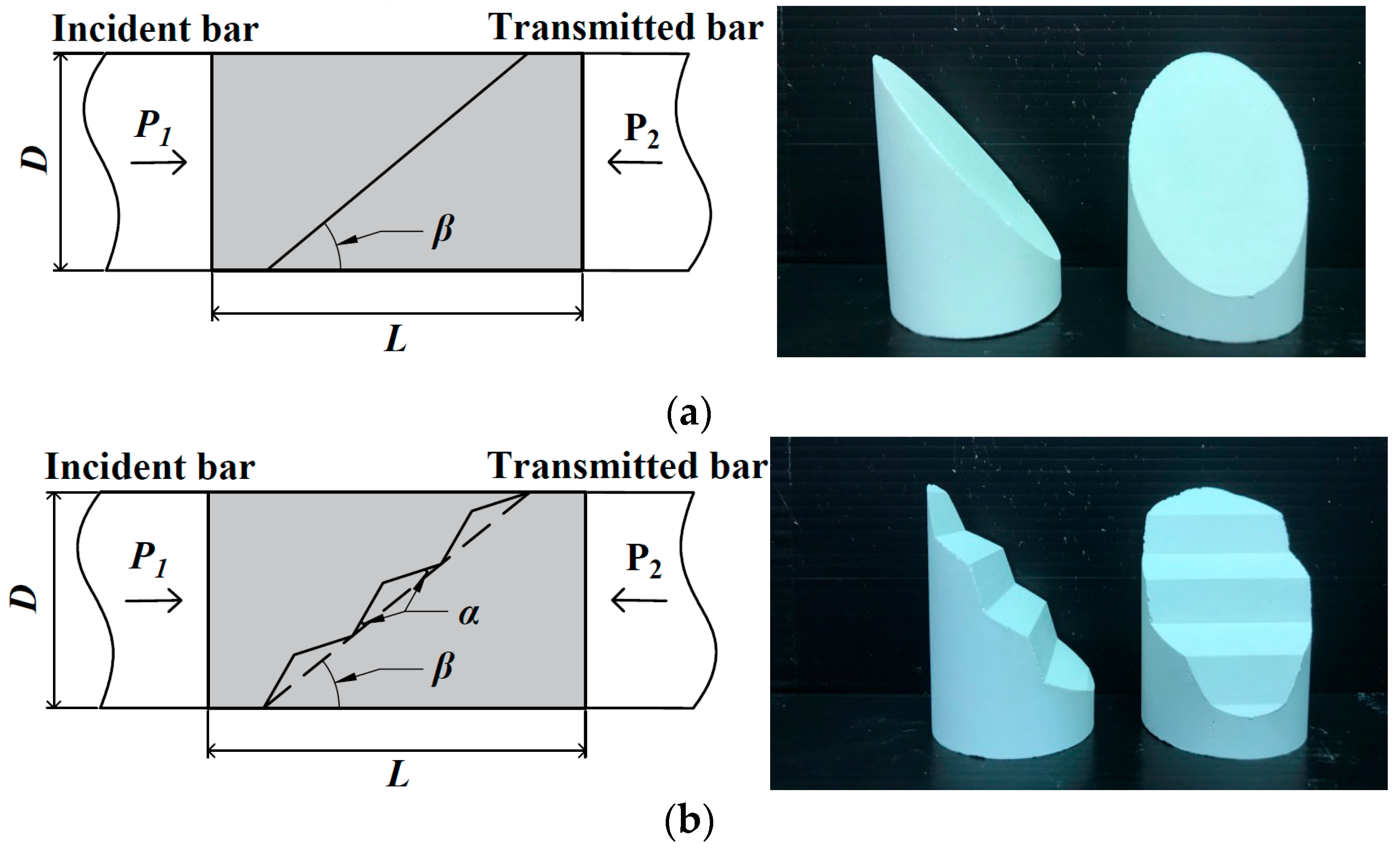
2.1. Preparation of Specimens

Man-made specimens of rock-like material, characterized by homogeneous properties, good tested stability, and normality, are produced by mixing gypsum powder, quartz powder, and pure water. All specimens are cylindrical with a diameter of 40 mm and a height of 70 mm. Figure 1 shows the specimens that contain a single planar joint and a joint with regularly triangular asperities, respectively. The included angle between the direction of load and the base plane of the joint, β, varies between 39° and 51°, with intervals of 6°, and the angle of asperity, α, varies between 0° and 21° in steps of 3°. The maximum angle β + α is 60°, and the minimum is 39°. For convenience of explanation, the specimens that contain a single planar joint and a joint with regularly triangular asperities are referred to herein as the planar joint specimen and the sawteeth joint specimen respectively, to distinguish them from the intact specimen without a joint. Obviously, the planar joint specimen is a special case of a sawteeth joint specimen with α = 0°. Notably, both sides of planar joint specimen and sawteeth joint specimen are closely contacted without infilled substance.
The man-made specimen is produced by mixing gypsum powder, quartz powder, and pure water in a weight ratio of 1:0.272:0.450 [33,35]. All specimens, each with a mass of about 140–150 g, are tested after seven days of curing. The standard deviation (SD) of the mass of 311 specimens is 2.35% of its mean value. The specimens have an average specific gravity of 2.02, a bulk density of 1.54 g/cm3, a porosity of 24.09%, and a water absorption ratio of 15.68%.
The uniaxial compressive strength (σUC) of the specimens is 15.31 ± 1.03 MPa, the tangential elastic modulus at half σUC (E50) is 16.31 ± 1.86 GPa, the Poisson’s ratio (v) is 0.285 ± 0.067, and the Brazilian tensile strength (σBT) is 2.49 ± 0.03 MPa. Accordingly, the strength ratio σUCBT = 6.15 and the modulus ratio E50/σUC = 1065. The rock-like specimen that was produced in this study can be used to imitate the engineering characteristics of rock with a high modulus ratio and a low strength, based on the classification method that was suggested by Deere [36].

2.2. Experimental Apparatus

Figure 2a shows the setup of the SHPB that is used in this study. In a rock dynamic test using a SHPB, the pressure of the gas chamber when the striker bar is released is typically regulated to generate various strain rates [21,22]. This method is utilized herein to provide strain rates of the incident bar within the range 83.1–259.0 s-1. Figure 3 plots the strain rates that are used in this study: these are generated in the SHPB by regulating the pressure of the gas chamber in the range 0.4–1.3 kg/cm2 while the striker bar is released. The stress can be determined from the Young’s modulus of the incident bar. Figure 3 plots both the stress increment per unit time and the strain rate. The loading rates that are generated in this study are in the range 3403–8467 GPa/s when no specimen is embedded between the incident bar and transmitted bar.
The applicability of the SHPB technique needs to be examined carefully before reliable dynamic experimental data can be obtained. The appearance of a discontinuity, for instance, the vacant one in-between the incident and transmitted bars, can interfere with the stress equilibrium during the application of dynamic impact since the mechanical impedance of the discontinuity is extremely small compared to that of solid bars and thus affects the dynamic stress propagation. Dynamic equilibrium is conventionally checked by comparing the transmitted signal and the difference between the incident and reflected signals [37]. The error, eε, can be evaluated by subtracting the measured strain that is generated by the transmitted wave from the sum of the strains that are generated by the incident wave and the back (reflected) wave at incidence: e ε = ε i ε r ε t . Only the dynamic equilibrium in early process during a SHPB test is concerned in this study since the failure of the embedded rock specimen leads to a non-equilibrium state. Therefore, the first waveforms of the recorded ε i ( t ) , ε r ( t ) , and ε t ( t ) are evaluated. The linearly increasing portion of recorded strain histories are extended to intercept the time axis to determine their corresponding arrival times, i.e., t 0 i , t 0 r , and t 0 t (Figure 2b). The time for incident pulse to reach its peak ( t p i ) is selected as half of the integration period, Δ t = ( t p i t 0 i ) , and the average error in the early dynamic equilibrium state is then determined as:
e ε = 1 2 Δ t t 0 j t 0 j + 2 Δ t ( ε i ε r ε r ) d t
where t 0 j are t 0 i , t 0 r , and t 0 t for the integration of ε i ( t ) , ε r ( t ) , and ε t ( t ) , respectively. The value of eε is in the range 0.5–51.9% (Figure 4).
The pressure measurement film (referred to as PMF herein) of the Fujifilm product is also adopted to examine the force equilibrium between the two ends of the specimen during a SHPB test (Figure 2a). Both low- and medium-pressure types of measurement film are used. Two PMFs of appropriate pressure scale are embedded between the two ends of specimen and the incident bar (the front PMF) and the transmitted bar (the rear PMF), respectively. Notably, only two PMFs are used in case no specimen is embedded. Table 1 illustrates typical results of some SHPB tests for various specimens under various pressures of the gas chamber while the strike bar is released. The area of PMF is decomposed into 64 parts to interpret corresponding densities of red patches and the average of these parts is used to represent the peak stress during the SHPB test. The peak stresses determined by two strain gauges installed respectively in the incident and transmitted bars are generally slightly higher than that by the PMF measured at the interface of the two bars. The linear regression lines between the peak stress and the released gas pressure are almost parallel with each other for these two stress measurement methods.
For an SHPB test with an embedded intact specimen, the densities of red patches reduce significantly. The front PMFs typically have slightly higher density than the rear PMF. The blank area in used PMFs appears only at low released gas pressures and is typically dispersed (Table 1). Linear regressive analysis shows that the difference in measured stresses varies insignificantly with the released gas pressure, indicating that both stress measurement methods are valid.
For a SHPB test with embedded planar joint or sawteeth joint specimens, the densities of red patches in the used PMFs under various released gas pressures are similar with that for intact specimen (Table 1). Uneven distribution of red patches in a pair of PMFs can be sometimes observed for a test with low released gas pressures. For such a condition, the difference in peak stresses determined from two PMFs and two gauges deviate by 20% or even more, and the two pieces of specimen slide relative to each other or partial fractured can be observed. The appearances of an inclined planar joint and sawteeth joint in a specimen, with appropriate assembly and close contact between its two parts, insignificantly change the mechanical impedance of the specimen under the SHPB testing condition in the study.
The force equilibrium condition during a SHPB test with and without an embedded specimen can be examined through the recorded strain histories or PMFs. The conventional strain gauge method is used hereinafter in this study. The peak stress determined during a SHPB test with non-equilibrium state caused by discontinuity in specimens, due to perhaps poor assembly of joint specimen and/or setup of a SHPB test, is not representative and will be screened out for study. Only results that are associated with an eε of less than 20.0% are utilized in subsequent analyses.

3. Results

Among the 311 prepared specimens, 210 specimens have eε < 20% (Figure 4). The failure type and dynamic peak stress of the specimens are discussed below.

3.1. Failure Type

After the SHPB test, each specimen is examined and is regarded as having failed if a fissure on its surface and sliding along its planar joint or triangular sawteeth joint are observed, if the specimen is fractured into many fragments, or if it is crushed into pieces. The specimens have various appearances after the test. Figure 5 shows six typical samples following the test. Figure 6 presents the three-dimensional (3D) appearances of some specimens. Obviously, the loading rate and the angle of the base plane (β) and the asperity (α) of a jointed specimen affect its failure. After the tests with low loading rates, an intact specimen may remain integrated with or without tiny flakes (Figure 5a), but the two parts of each jointed specimen in a test can slide relative to each other, with both parts remaining intact (Figure 5b) or only minor scratches on their surface (Figure 5c,g,h). Most specimens lose their integrity at a high loading rate (Figure 5e,f). The specimens with a small magnitude of β + α at a low loading rate are prone to slide failure, while the specimens with a large magnitude of β + α, or subjected to a high loading rate, are typically crushed.
Figure 7 plots the distributions of the sizes of particles in some of the specimens after testing. Based on the distribution of particle sizes in Figure 7, Table 2 classifies the types of failure of the specimens after the SHPB test as follows: (A) intact with or without tiny flakes, (B) slide failure, (C) fracture failure, and (D) crushing failure. Type C can be divided into the following two subtypes: (C1) broken along the concave of the sawteeth, and (C2) complete fracture.
Table 3 lists the types of failure of all tested specimens based on the classification in Table 2. Specimens with β = 39°, 45°, and 51°, apart from the intact specimen, have two parts that can slide relative to each other until failure. At a particular loading rate, the two parts of a specimen that have a smaller β are more apt to slide relative to each other and are severely fractured if it happens. A specimen that has greater α is more likely to be fractured or crushed to failure. Among specimens with similar total angles of the base plane and asperity (β + α), only those with α ≤ 6° have two parts that slide relative to each other and have irregular fragments if fractured. In contrast, those with α > 6° do not exhibit sliding but break to failure. Broken fragments are commonly observed in the recessions of the sawteeth of a specimen and are associated with partial cut-off sawteeth as well as striations and shear marks on the surface of the sawteeth.

3.2. Dynamic Peak Stress

Three peaks in first waveforms of corresponding ε i ( t ) , ε r ( t ) , and ε t ( t ) in Figure 2b, denoted as ε i p , ε r p , and ε t p , are used to determine the dynamic peak stress, which is considered to be the dynamic strength of the specimen.
Figure 8 and Figure 9 plot the dynamic peak stresses of the intact specimen and the jointed specimen that are obtained at various loading rates in the SHPB test. The dynamic peak stress of the intact specimen increases almost linearly with loading rate, and the variation of the dynamic peak stress becomes obvious at high loading rates (Figure 8a).
Figure 8b,c plots the dynamic peak stress of the jointed specimens with β = 39° and β = 45° at various loading rates. The two parts of the specimens that contain a single planar joint with β = 39° and 45° (α = 0°) (Figure 9a,b) exhibit relative movement of both sides of the planar joint after testing at a loading rate of less than 1601.4 ± 463.9 GPa/s. When the loading rate exceeds 1830.9 ± 425.7 GPa/s, the specimen is fractured or even crushed to failure. As the loading rate increases, the dynamic peak stress of the specimen also increases. This increase in the dynamic peak stresses with loading rate of the specimen with β = 45°and α = 0°, exceeds that of the specimen with β = 39°and α = 0°.
Figure 8d plots the dynamic peak stress of specimen with β = 51° at various loading rates. As in the planar joint specimens with β = 39° and β = 45°, the two parts of the specimens with β = 51° (and α = 0°) (Figure 9c) slide relative to each other during the test at a loading rate of 936.1 ± 453.8 GPa/s. Both slide failure and fracture failure of specimens are observed after testing at a loading rate of 1601.4 ± 463.9 GPa/s. As the loading rate increases, the specimen is fractured and crushed, with its dynamic peak stress increasing from 35.82 ± 25.02 to 75.32 ± 17.60 MPa. The increase in dynamic peak stress is smaller than those of specimens with β = 39°, α = 0° and β = 45°, α = 0°.
The failure type and dynamic peak stress of the specimen with β = 39° with gently triangular sawteeth asperities, α < 6°, resemble those of the planar joint specimen (β = 39°, α = 0°) with a greater variation in dynamic peak stress (42.26 ± 24.48 MPa – 96.39 ± 16.28 MPa). When the triangular sawteeth asperity becomes large, α > 6°, sliding between the two parts of each specimen is prevented. The asperities of the specimen are sheared off or the specimen breaks at a loading rate of less than 1601.4 ± 463.9 GPa/s. When the loading rate exceeds 1830.9 ± 425.7 GPa/s, most specimens are fractured to failure, but the specimen with β = 39° and α = 21° is crushed. The dynamic peak stress of all specimens increases from 57.67 ± 18.12 to 91.75 ± 17.44 MPa.
The failure type and dynamic peak stress of the specimen with β = 45° with gently triangular sawteeth asperities, α < 6°, resemble those of the planar joint specimen (β = 45°, α = 0°), and slide failure is observed after testing at a low loading rate. As the loading rate increases, the specimen becomes fractured or even crushed to failure. The increases in dynamic peak stress (23.42 ± 15.81 MPa – 85.22 ± 17.56 MPa) are also similar, with limited variation. When the triangular sawteeth asperity becomes is large, α > 6°, sliding between the two parts of the specimens is prevented. The specimen is fractured to failure at a loading rate of less than 1601.4 ± 463.9 GPa/s, and is crushed when the loading rate exceeds 2211.4 ± 615.8 GPa/s. The dynamic peak stress of the specimens increases from 75.23 ± 15.02 to 89.49 ± 32.52 MPa.
Slide failure of the specimen with β = 51° with gently triangular sawteeth asperities (α < 6°) can be observed after testing at a loading rate of 936.1 ± 453.8 GPa/s. As the loading rate increases, the specimen is fractured or even crushed to failure and the dynamic peak stress increases from 23.76 ± 10.89 to 78.48 ± 21.94 MPa. When the triangular sawteeth asperity becomes large, α > 6°, sliding between the two parts of specimens is prevented. The specimen is fractured to failure when the loading rate is less than 1830.9 ± 425.7 GPa/s, and it is crushed when the loading rate exceeds 2211.4 ± 615.8 GPa/s. The dynamic peak stress also increases from 61.68 ± 19.48 to 81.23 ± 17.59 MPa.

4. Discussion

Based on the failure type and dynamic peak strength of specimens that are obtained from the SHPB test, the factors that affect the dynamic behaviors of a specimen that contains various joint patterns are discussed below.

4.1. Appearance of Joint

The dynamic peak stresses of both the intact specimen and the jointed specimen increase with the loading rate in the range 303.1–5233.6 GPa/s. However, their relationships between dynamic peak stress and loading rate differ from each other. Based on failure types in Table 3, Figure 8a and Figure 9 show the dynamic peak stresses and associated failure types for the intact specimen and the planar joint specimen at various loading rates. The appearance of a joint plane enables slide failure, so the dynamic peak stress of the jointed specimens as slide failure is lower than that of the intact specimens. The joint plane in specimens also reduces their dynamic peak strength at fracture failure, revealing that the presence of a joint in rocks affects not only their static strength but also their dynamic peak strength. Notably, upon crushing failure, the appearance of a joint plane can reduce the lower bound but not the upper bound on the dynamic peak strength, indicating that the influence of the joint becomes insignificant when the loading rate is sufficiently increased.
Linear regression analysis was performed for the quantitative relationship between the dynamic peak stress and loading rate for each intact specimen and jointed specimen with distinct base angles. Table 4 lists linear equations of regression and associated coefficients of determination. The intact specimen is able to endure the impact of a loading rate of up to 3354.3 GPa/s, its measured dynamic peak stress increases steeply with loading rate, and the corresponding slope exceeds those of planar joint specimens that have fracture failure (Table 4). The slope for planar joint specimens with a fracture failure is greater than that for specimens with slide failure but is less than that for intact specimens with fracture failure. Similarly, the appearance of joint plane in a specimen that is crushed to failure reduces the slope of the relationship between dynamic peak strength and applied loading rate, and the influence is insignificant relative to the specimens that are fractured to failure. The experimental results are consistent with those of Shu et al. [35].

4.2. ANOVA on Factors that Affect Dynamic Peak Strength of Jointed Specimen

Statistical analysis of variance (ANOVA) was carried out to identify the factors that affect the dynamic behaviors of a specimen that contains various joint patterns and to facilitate subsequent investigation. The loading rate, β, and α were selected as the independent variables and the dynamic peak stress that was obtained in the SHPB test is the dependent variable. The independent variables were normalized using their respective average values and standard deviations since the magnitude of the loading rate is much greater than those of β and α. ANOVA was separately performed on the results of slide failure, fracture failure, and crushing failure to eliminate any effect of failure type.
A total of 36, 112, and 47 data associated with slide failure, fracture failure, and crush failure were obtained after the SHPB tests. Table 5 lists the results of the ANOVA for specimens with fracture failure. The statistical F value is very high, indicating that variations in repeated treatments (experimental groups with the same independent variables) are significantly smaller than those among various treatments with different independent variables: this fact permits an examination of the influence of each independent variable. For the jointed specimens that fail by fracture, the test statistics of the loading rate, β, and α all exceed the thresholds for rejection at a 90% level of significance, and the p-values are all less than 0.10 (Table 5), indicating that all of these factors significantly affect the dynamic peak stresses of jointed specimen in a SHPB test. Table 6 lists the significant factors affecting the dynamic peak strength for various failure types. For the jointed specimens with slide failure, the loading rate and β are significantly affected factors, and for the jointed specimens that are crushed to failure, the loading rate is the only significantly affected factor.

4.3. Pattern of Joints

Results of the SHPB test for the planar joint specimen and the sawteeth joint specimen reveal the influence of joint pattern on the dynamic characteristics of a jointed rock mass. Figure 10 plots the dynamic peak stresses for jointed specimens that have total angles of β + α = 45° and 51°. The maximum angle of application of the load to the joint surface for the sawteeth joint specimen that has β = 39° and α = 6°equals that for the planar joint specimen with a joint angle of 45°. Nevertheless, these two specimens have different outcomes (Figure 10a). When slide failure occurs, the planar joint specimen exhibits a lower slope of the relationship between the dynamic peak stresses and loading rate than those of the sawteeth joint specimen. The upper bound on the loading rate that causes sliding between the two parts of the planar joint specimen is also lower than that of the sawteeth joint specimen. When fracture failure happens, the slope of the relationship between the dynamic peak stress and the loading rate for the planar joint specimen is close to that for the sawteeth joint specimen (Table 4).
The sawteeth joint specimen that has β = 45° and α = 6° and the planar joint specimen with a joint angle of 51° yields similar results. The planar joint specimen has a smaller slope of the relationship between the dynamic peak stresses and loading rate, and a lower upper bound on the loading rate that causes slide failure. The planar and the sawteeth joint specimens have similar slopes of the relationship between the dynamic peak stresses and loading rate when fracture failure happens (Figure 10b and Table 4). Remarkably, the sawteeth joint specimen with β = 39° and α = 12° fails only by fracture and not by sliding at a low loading rate. These experimental results indicate that the combination of β and α angles influence not only the relationship between the dynamic peak stresses and loading rate, but also the failure types of jointed specimen under various loading rates, for a particular maximum angle of application of the load to the joint surface of the specimen. The triangular sawteeth with an asperity angle of 6° provides more friction than the planar joint with a similar angle of loading, leading to a higher dynamic peak stress when slide failure occurs.

4.4. Angle of Triangular Sawteeth

Figure 11 shows a box-and-whisker plot of the dynamic peak stress at various angles, α, for the specimen with β = 39°, 45°, and 51°. For the specimen with β = 39° (Figure 11a), the middle 50% of the box that represents the dynamic peak stress due to crushing failure, the dynamic peak stress is typically higher than those caused by slide failure and fracture failure, especially for α = 0°, 3°, and 6°, revealing that the dynamic peak stress of the specimen dominated by crushing failure differs from those by other failure types. The dynamic peak stress in the middle part of the box that is associated with crushing failure of the specimens with β = 45° and 51° partially overlaps those in boxes associated with other failure types (Figure 11b,c). The differences in the dynamic peak stresses that are dominated by various failure types are not great. However, for a particular α angle, the mean dynamic peak stress of a specimen due to slide failure is lowest, to fracture failure is second lowest, and to crushing failure is highest.
Figure 12 shows the box-and-whisker plot of the ratio of dynamic peak stress to loading rate (DSLR) at various α angles for the specimen with β = 39°, 45°, and 51°. Typical DSLR values are in the range 0.02–0.08. In contrast to Figure 11, for the specimens that have the same α angle but exhibit different failure types, the dynamic peak stress in the middle 50% of the box that represents dynamic peak stress due to crushing failure is typically lower than those due to slide failure and fracture failure. These results indicate that increasing the loading rate increases the dynamic peak stress of a jointed specimen upon slide failure and fracture failure. The mean DSLR value for a specimen that fails by fracture is typically lower than that of specimen that undergoes slide failure and has the same angle, α. However, the middle parts of their corresponding boxes have similar DSLR values, indicating variations in the relationship between DSLR value and loading rate.
Figure 13 plots the change in the DSLR with the α angle for the specimen with β = 39°. When slide failure or fracture failure occurs, the DSLR increases linearly with α, with coefficients of determination, R2, of 0.688 and 0.886 respectively, revealing medium to high correlations. However, when crushing failure happens, the coefficient of determination for the linear regression between the DSLR and α is very low, indicating that the angle, α, is not a significant factor under such a condition. Similar results are obtained for specimens with β = 45° and 51°. Increasing α increases the DSLR of the jointed specimen, but this effect is further influenced by the β angle of the specimen and its associated failure type.

4.5. Loading Rate

The results of the SHPB test indicate that the dynamic peak stress of specimen increases with the loading rate, regardless of the appearance of the joint, the angles of base plane and sawteeth of the joint, and the type of failure type of the specimen. The rate of increase of the dynamic peak stress typically decreases as the loading rate increases. When the jointed specimen is crushed to failure, the applied load is dissipated by the whole specimen. The DSLR value is moderately negatively correlated with the loading rate: increasing the loading rate reduces the efficiency of increase of the dynamic peak stress. If the specimen is broken by fracture, then the applied load is mostly dissipated by a small number of fracture surfaces, so the rate of increase of the dynamic peak stress is lower than that of a specimen under crushing failure. The concentration of stress on a few fracture surfaces, where it is affected by the angles β and α, causes variation in the relationship between the DSLR and loading rate. Therefore, the results of ANOVA indicate that both β and α angles affect the dynamic peak stress of a jointed specimen that fails by fracture. The joint across the whole specimen in the direction of the base plane causes β to affect the dynamic peak stress of the jointed specimen when slide failure occurs. The stresses on both sides of the triangles of sawteeth that are caused by the applied load vary greatly, accounting for the fact that the influence of α on the dynamic peak stress of a jointed specimen is insignificant. The dynamic peak stress of the jointed specimen increases with loading rate, but the rate of increase is significantly lower than for specimens under fracture failure or crushing failure, and the DSLR varies considerably with the loading rate, so ANOVA and simple regression cannot quantify these relationships.

5. Conclusions

In this study, intact rock-like specimens and specimens with closely contacted regular asperities at various angles are prepared for SHPB testing. The effects of loading rate, angle of base plane, and asperity on the dynamic peak stress/strength of the specimens are examined. The following conclusions are drawn.
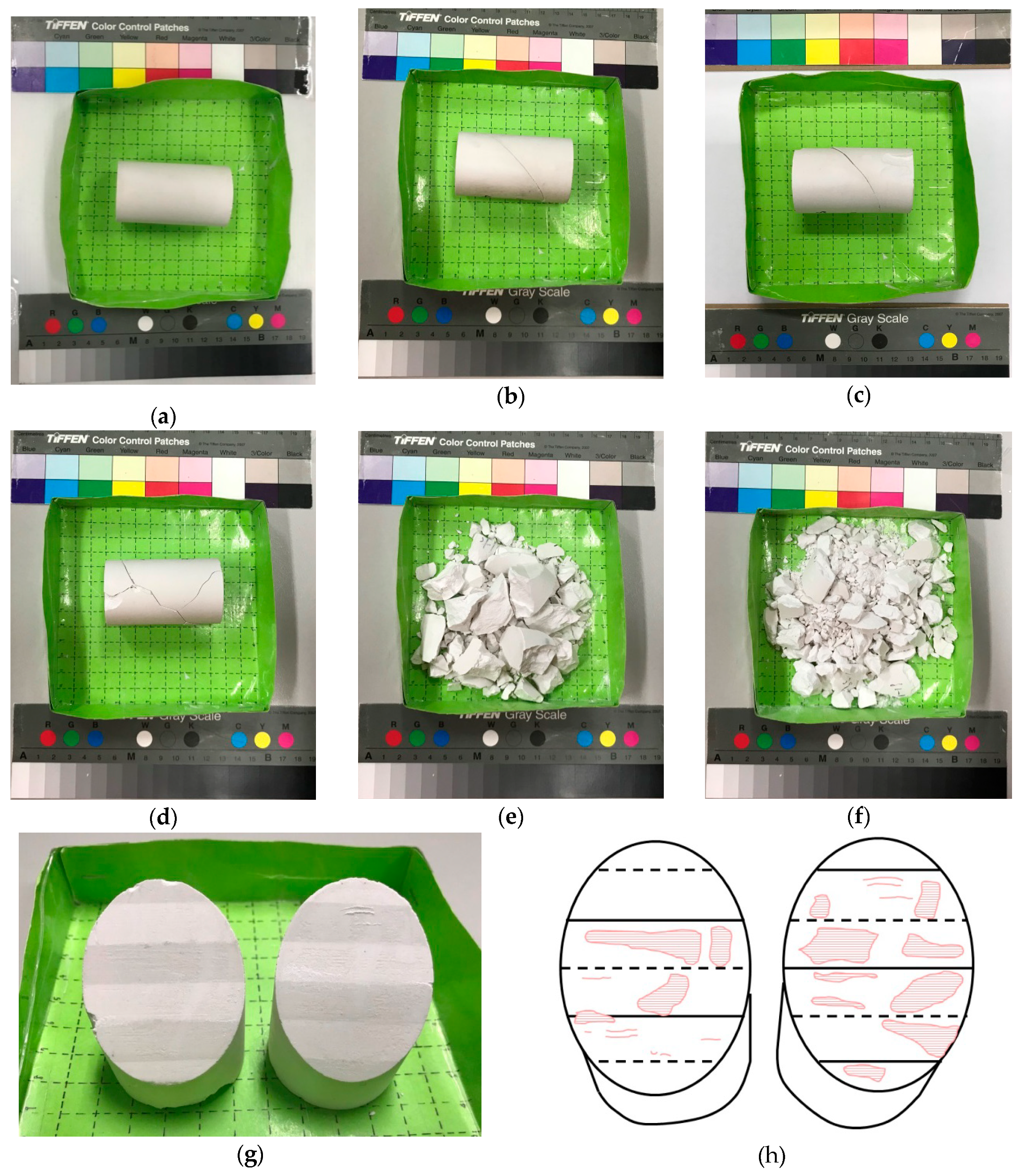
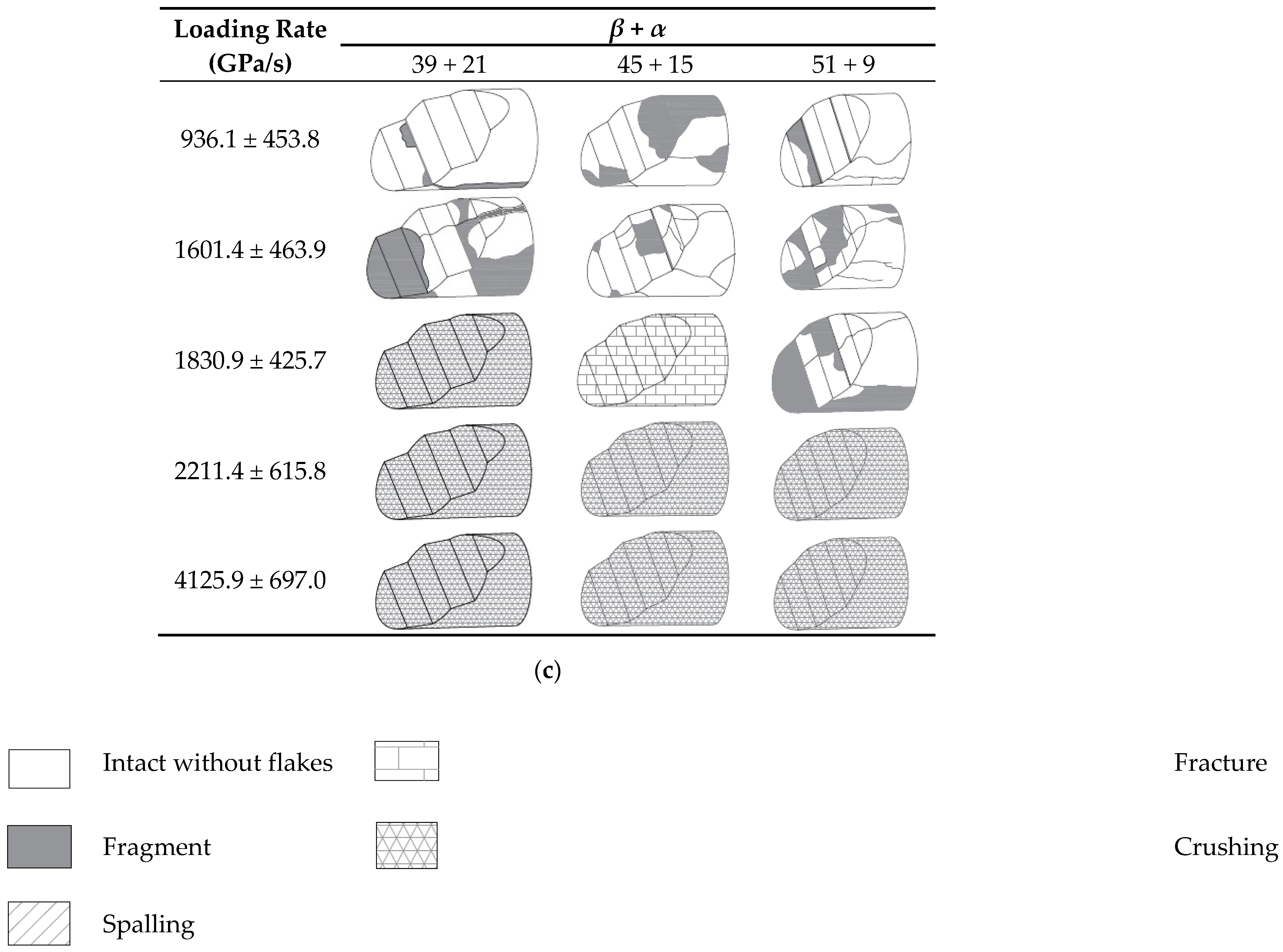
  • The appearance of a joint makes the outcomes for a specimen in an SHPB test more diverse. The failures of an intact specimen and a jointed specimen can be classified into the following four types: (A) intact with or without tiny flakes, (B) slide failure, (C) fracture failure, and (D) crushing failure. Therefore, the relationship between dynamic peak stress and loading rate varies greatly.
  • The results of ANOVA indicate that the loading rate, the angle of the base plane (β), and asperity (α) all affect the dynamic peak stress of jointed specimens when fracture failure occurs. When slide failure occurs, the dynamic peak stress of the jointed specimen is affected by loading rate and β, when the specimen is crushed to failure, the loading rate is the sole factor that significantly influences its dynamic peak stress.
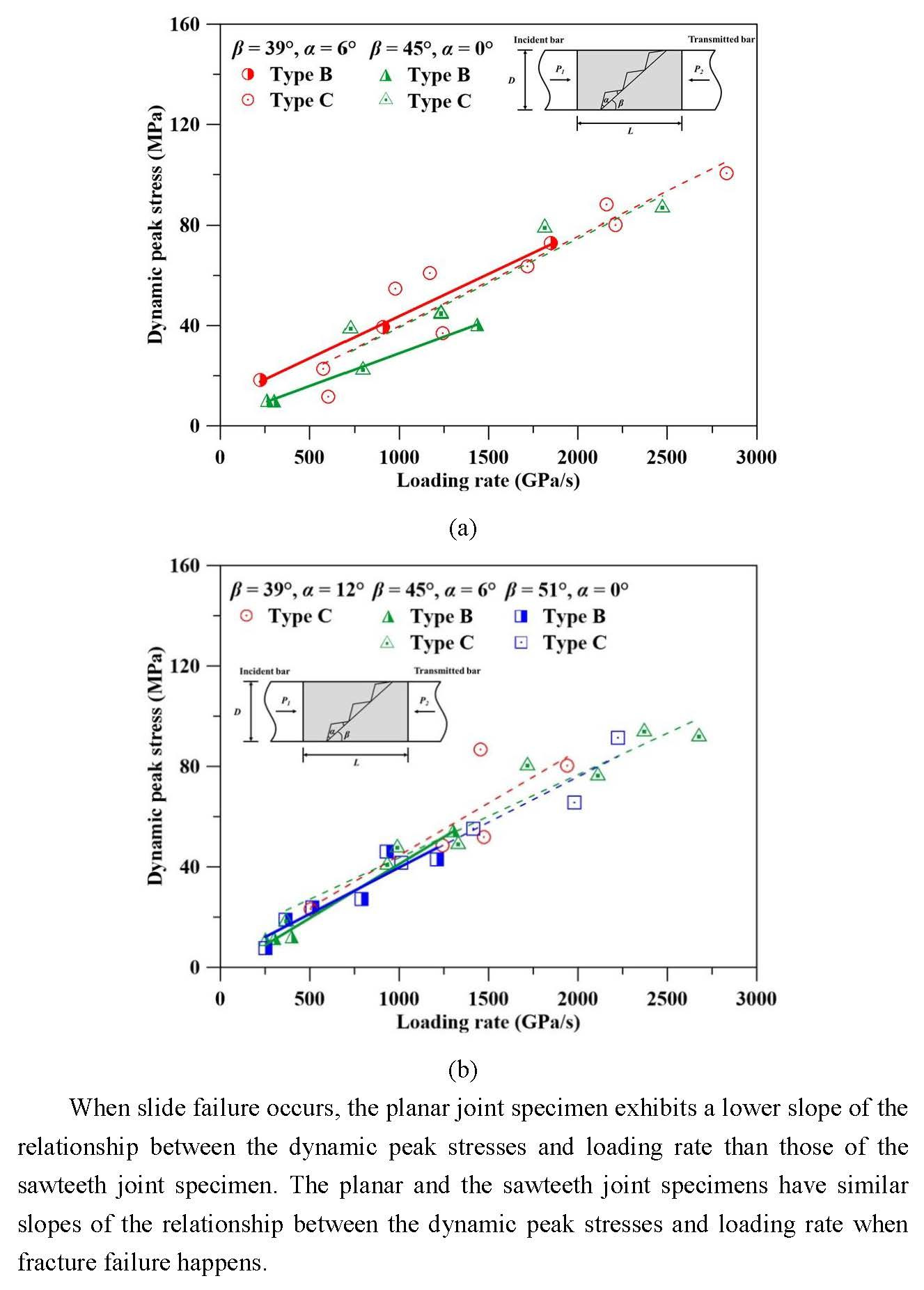
  • The slope of the relationship between the dynamic peak stress and the loading rate, and the upper limit of the dynamic peak stress under slide failure of the planar joint specimen, are both smaller than those of the sawteeth joint specimen when the loads that are applied on joint surface have similar maximum angles. The slope of the relationship between the dynamic peak stress and the loading rate under fracture failure for the planar joint specimen is close to that for the sawteeth joint specimen. The small sawtooth with α ≤ 6° provides additional friction on the surface of jointed specimen under slide failure. No slide failure is observed for the specimen with α > 6°.
  • Increasing angle α increases the DSLR of the jointed specimen at slide failure, and this effect is influenced by the angle β of the specimen and the associated failure type. The angle α insignificantly affects the DSLR when the jointed specimen is crushed to failure.
  • The dynamic peak stress of a specimen increases with the loading rate at a gradually decreasing rate. The β and α of the jointed specimen affect the location of stress concentration during loading, further influencing the dynamic peak stress for specimens under slide failure and fracture failure. When the loading rate is high and the specimen is crushed to failure, the influences of β and α disappear. Increasing the loading rate reduces the efficiency of increase of dynamic peak stress.

Author Contributions

T.-T.W.; Formal analysis, P.-Y.S.; Funding acquisition, T.-T.W.; Investigation, P.-Y.S. and C.-Y.L.; Project administration, P.-Y.S.; Resources, H.-H.L., T.-W.C. and T.-H.U.; Validation, P.-Y.S.; Writing – original draft, P.-Y.S.; Writing – review & editing, T.-T.W. All authors provided critical feedback and helped shape the research, analysis and manuscript. All authors have read and agreed to the published version of the manuscript.

Funding

This research received no external funding.

Acknowledgments

The authors would like to thank the Ministry of Science and Technology, Taiwan, for financially supporting this research under contracts NSC 102-2221-E-027-071-MY3 and MOST-105-2116-M- 027-002.

Conflicts of Interest

The authors declare no conflict of interest.

References

  1. Rehbock-Sander, M.; Jesel, T. Fault induced rock bursts and micro-tremors-experiences from the Gotthard Base Tunnel. Tunn. Undergr. Space Technol. 2018, 81, 358–366. [Google Scholar] [CrossRef]
  2. Kung, C.L.; Wang, T.T.; Chen, C.H.; Huang, T.H. Response of a circular tunnel through rock to a harmonic Rayleigh wave. Rock Mech. Rock Eng. 2018, 51, 547–559. [Google Scholar] [CrossRef]
  3. Chao, W.A.; Wu, Y.M.; Zhao, L.; Chen, H.; Chen, Y.G.; Chang, J.M.; Lin, C.M. A first near real-time seismology based landquake monitoring system. Sci. Rep. 2017, 7, 1–12. [Google Scholar] [CrossRef] [Green Version]
  4. Ku, C.S.; Kuo, Y.T.; Chao, W.A.; You, S.H.; Huang, B.S.; Chen, Y.G.; Taylor, F.W.; Wu, Y.M. A first-layered crustal velocity model for the western Solomon Islands: Inversion of the measured group velocity of surface waves using ambient noise. Seismol. Res. Lett. 2018, 89, 2274–2283. [Google Scholar] [CrossRef]
  5. Pal, S.; Kaynia, A.M.; Bhasin, R.K.; Paul, D.K. Earthquake stability analysis of rock slopes: A case study. Rock Mech. Rock Eng. 2012, 45, 205–215. [Google Scholar] [CrossRef]
  6. Kumsar, H.; Aydan, Ö.; Ulusay, R. Dynamic and Static Stability Assessment of Rock Slopes Against Wedge Failures. Rock Mech. Rock Eng. 2000, 33, 31–51. [Google Scholar] [CrossRef]
  7. Wang, Z.; Tian, N.; Wang, J.; Liu, J.; Hong, L. Experimental Study on Damage Mechanical Characteristics of Heat-Treated Granite under Repeated Impact. J. Mater. Civ. Eng. 2018, 30, 04018274. [Google Scholar] [CrossRef]
  8. Mishra, S.; Chakraborty, T.; Matsagar, V.; Loukus, J.; Bekkala, B. High Strain-Rate Characterization of Deccan Trap Rocks Using SHPB Device. J. Mater. Civ. Eng. 2018, 30, 04018059. [Google Scholar] [CrossRef]
  9. Aydan, Ö. Rock Dynamics; ISRM Book Series; CRC Press: Boca Raton, FL, USA, 2017. [Google Scholar]
  10. Liu, S.; Xu, J.Y. Effect of strain rate on the dynamic compressive mechanical behaviors of rock material subjected to high temperatures. Mech. Mater. 2015, 82, 28–38. [Google Scholar] [CrossRef]
  11. Török, Á.; Ficsor, A.; Davarpanah, M.; Vásárhelyi, B. Comparison of Mechanical Properties of Dry, Saturated and Frozen Porous Rocks. In Proceedings of the IAEG/AEG Annual Meeting Proceedings, San Francisco, CA, USA, 17–21 September 2018. [Google Scholar]
  12. Mastrorocco, G.; Salvini, R.; Vanneschi, C. Fracture mapping in challenging environment: A 3D virtual reality approach combining terrestrial LiDAR and high definition images. Bull. Eng. Geol. Environ. 2018, 77, 691–707. [Google Scholar] [CrossRef] [Green Version]
  13. Zhan, S.S.; Wang, T.T.; Huang, T.H. Variations of hydraulic conductivity of fracture sets and fractured rock mass with test scale: Case study at Heshe well site in central Taiwan. Eng. Geol. 2016, 206, 94–106. [Google Scholar] [CrossRef]
  14. Liu, X.J.; Zheng, X.; Cheng, W.C.; Kong, Q.; Wang, J.J. The shear strength of the nature loess joint: A Case study in Shaanxi Province. J. Test. Eval. 2019, 47, 2297–2312. [Google Scholar] [CrossRef]
  15. Tian, Y.C.; Liu, Q.S.; Ma, H.; Liu, Q.; Deng, P.H. New peak shear strength model for cement filled rock joints. Eng. Geol. 2018, 233, 269–280. [Google Scholar] [CrossRef]
  16. He, S.Y. Experimental Study of Crack Propagation Law of Shale Containing Prefabricated Fractures. Adv. Civ. Eng. Mater. 2018, 7, 558–575. [Google Scholar] [CrossRef]
  17. Jiang, Y.F.; Wang, L.Q.; Wu, Q.; Sun, Z.; Elmo, D.; Zheng, L.B. An improved shear stress monitoring method in numerical direct shear tests by Particle Flow Code. J. Test. Eval. 2020, 48. [Google Scholar] [CrossRef]
  18. Chiu, C.C.; Weng, M.C.; Huang, T.H. Modeling rock joint behavior using a rough-joint model. Int. J. Rock Mech. Min. Sci. 2016, 89, 14–25. [Google Scholar] [CrossRef]
  19. Kazerani, T.; Yang, Z.Y.; Zhao, J. A discrete element model for predicting shear strength and degradation of rock joint by using compressive and tensile test data. Rock Mech. Rock Eng. 2012, 45, 695–709. [Google Scholar] [CrossRef] [Green Version]
  20. Wang, Z.L.; Li, H.R.; Wang, J.G.; Shi, H. Experimental study on mechanical and energy properties of granite under dynamic triaxial condition. Geotech. Test. J. 2018, 41, 1063–1075. [Google Scholar] [CrossRef]
  21. Xia, K.W.; Yao, W. Dynamic rock tests using split Hopkinson (Kolsky) bar system—A review. J. Rock Mech. Geotech. Eng. 2015, 7, 27–59. [Google Scholar] [CrossRef] [Green Version]
  22. Zhang, Q.B.; Zhao, J. A review of dynamic experimental techniques and mechanical behaviour of rock materials. Rock Mech. Rock Eng. 2014, 47, 1411–1478. [Google Scholar] [CrossRef] [Green Version]
  23. Pyrak-Nolte, L.J.; Myer, L.R.; Cook, N.G.W. Transmission of seismic waves across single natural fractures. J. Geophys. Res. 1990, 95, 8617–8638. [Google Scholar] [CrossRef]
  24. Zhao, J.; Cai, J.G. Transmission of elastic P-waves across single fractures with a nonlinear normal deformational behavior. Rock Mech. Rock Eng. 2001, 34, 3–22. [Google Scholar] [CrossRef]
  25. Li, M.; Qiao, L.; Li, Q.W. Energy dissipation of rock specimens under high strain rate with single joint in SHPB tensile tests. Chin. J. Geotech. Eng. 2017, 39, 1336–1343. [Google Scholar]
  26. Rong, L.; Li, J.; Li, H.; Li, Z.; Hong, S. Measurement of seismic quality factor of jointed rock based on stress wave energy. Chin. J. Rock Mech. Eng. 2017, 36, 2474–2483. [Google Scholar]
  27. Li, J.C.; Li, N.N.; Li, H.B.; Zhao, J. An SHPB test study on wave propagation across rock masses with different contact area ratios of joint. Int. J. Impact Eng. 2017, 105, 109–116. [Google Scholar] [CrossRef]
  28. Wang, G.; Zhang, X.P.; Jiang, Y.J.; Wu, X.Z.; Wang, S.G. Rate-dependent mechanical behavior of rough rock joints. Int. J. Rock Mech. Min. Sci. 2016, 83, 231–240. [Google Scholar] [CrossRef]
  29. Atapour, H.; Moosavi, M. The influence of shearing velocity on shear behavior of artificial joints. Rock Mech. Rock Eng. 2014, 47, 1745–1761. [Google Scholar] [CrossRef]
  30. Yang, Z.Y.; Chiang, D.Y. An experimental study on the progressive shear behavior of rock joints with tooth-shaped asperities. Int. J. Rock Mech. Min. Sci. 2000, 37, 1247–1259. [Google Scholar] [CrossRef]
  31. Wu, W.; Li, J.C.; Zhao, J. Loading rate dependency of dynamic responses of rock joints at low loading rate. Rock Mech. Rock Eng. 2012, 45, 421–426. [Google Scholar] [CrossRef] [Green Version]
  32. Liu, X.R.; Kou, M.M.; Lu, Y.M.; Liu, Y.Q. An experimental investigation on the shear mechanism of fatigue damage in rock joints under pre-peak cyclic loading condition. Int. J. Fatigue 2018, 106, 175–184. [Google Scholar] [CrossRef]
  33. Li, H.H. Mechanical Responses of rock joints with regular asperities under various shear rates investigated by double shear test. J. Test. Eval. 2017, 45, 470–483. [Google Scholar] [CrossRef]
  34. Zhou, L.J.; Xu, S.L.; Shan, J.F.; Liu, Y.G.; Wang, P.F. Heterogeneity in deformation of granite under dynamic combined compression/shear loading. Mech. Mater. 2018, 123, 1–18. [Google Scholar] [CrossRef]
  35. Shu, P.Y.; Li, H.H.; Wang, T.T.; Ueng, T.H. Dynamic strength of rock with single planar joint under various loading rates at various angles of loads applied. J. Rock Mech. Geotech. Eng. 2018, 10, 545–554. [Google Scholar] [CrossRef]
  36. Deere, D.U. Geological considerations. In Rock Mechanics in Engineering Practice; Stagg, K.G., Zienkiewicz, O.C., Eds.; Wiley: New York, NY, USA, 1968; pp. 1–20. [Google Scholar]
  37. Song, B.; Chen, W. Dynamic stress equilibration in split Hopkinson pressure bar tests on soft materials. Exp. Mech. 2004, 44, 300–312. [Google Scholar] [CrossRef]
Figure 1. Specimens that contain a single planar joint (a) and a joint with regular triangular sawteeth asperities (b). D and L are the diameter and height of specimen, respectively. P1 and P2 are the loading directions of pressure.
Applsci 10 05204 g001
Figure 2. Setup of experiment with the Split Hopkinson Pressure Bar (SHPB) test (a) and interpretation on measured waveforms of strain histories (b).
Applsci 10 05204 g002
Figure 3. Relationship between pressure of gas chamber when striker bar is released and loading rate.
Applsci 10 05204 g003
Figure 4. Average error (eε) in early dynamic equilibrium state for all SHPB tests in this study. 210 of 311 specimens have eε < 20%. Plot of eε with gas pressure.
Applsci 10 05204 g004
Figure 5. Images of specimen after the SHPB test: (a) integrated without any flaking of intact specimen, (b) two parts of specimen, with β = 39° and α = 0° slide relative to each other, without any tiny flakes, (c) two parts of specimen, with β = 51° and α = 3° slide relative to each other, with tiny flakes on both parts, (d) fractured specimen, with β = 39° and α = 18°, break along concave part of sawteeth can be observed, (e) completely fractured specimen, with β = 45° and α = 15°, (f) crushed jointed specimen, (g) scratches on joint surface of specimen in (c), (h) depicting (g) with an emphasis on scratches on joint surface.
Applsci 10 05204 g005
Figure 6. Three-dimensional (3D) sketch of representative specimens after the SHPB test, (a) α = 0°, (b) β + α = 45°, (c) β + α = 60°.
Applsci 10 05204 g006aApplsci 10 05204 g006b
Figure 7. Size distribution of particles in specimens after the SHPB test.
Applsci 10 05204 g007
Figure 8. Relationship between dynamic peak stress/strength and loading rate of intact specimen (a) and all jointed specimens with β = 39°, 45°, and 51° (bd).
Applsci 10 05204 g008
Figure 9. Relationship between dynamic peak stress/strength and loading rate of planar joint specimens with β = 39°, 45°, and 51° (ac).
Applsci 10 05204 g009
Figure 10. Relationship between dynamic peak stress/strength and loading rate of specimens with similar maximum angles of application of load on joint surface. (a) β = 45°, α = 0° versus β = 39°, α = 6°, (b) β = 51°, α = 0° versus β = 45°, α = 6° and β = 39°, α = 12°.
Applsci 10 05204 g010
Figure 11. Box-and-whisker plot of dynamic peak stress at various angles, α, for specimens with β = 39°, 45°, and 51°(ac).
Applsci 10 05204 g011
Figure 12. Box-and-whisker plot of ratio of dynamic peak stress to loading rate (DSLR) at various angles, α, for specimens with β = 39°, 45°, and 51°(ac).
Applsci 10 05204 g012
Figure 13. Change in DSLR with the angles, α, of specimen with β = 39°.
Applsci 10 05204 g013
Table 1. Illustration of red patches on pressure measurement films (PMFs) used between interfaces of embedded specimen and incident and transmitted bars in a SHPB test. Medium-pressure types are used except low-pressure type is used in the four on the right of the last row, with gray background.
Gas Pressure
(kg/cm2)
No SpecimenIntact SpecimenPlanar Joint SpecimenSawteeth Joint Specimen
Front PMFRear PMFFront PMFRear PMFFront PMFRear PMF
0.8–1.3 Applsci 10 05204 i001 Applsci 10 05204 i002 Applsci 10 05204 i003 Applsci 10 05204 i004 Applsci 10 05204 i005 Applsci 10 05204 i006 Applsci 10 05204 i007
0.5–0.7 Applsci 10 05204 i008 Applsci 10 05204 i009 Applsci 10 05204 i010 Applsci 10 05204 i011 Applsci 10 05204 i012 Applsci 10 05204 i013 Applsci 10 05204 i014
0.3–0.4 Applsci 10 05204 i015 Applsci 10 05204 i016 Applsci 10 05204 i017 Applsci 10 05204 i018 Applsci 10 05204 i019 Applsci 10 05204 i020 Applsci 10 05204 i021
Applsci 10 05204 i022 Applsci 10 05204 i023 Applsci 10 05204 i024 Applsci 10 05204 i025 Applsci 10 05204 i026 Applsci 10 05204 i027 Applsci 10 05204 i028
Table 2. Description for each failure type.
Failure Type SubtypeGrain Size Distribution RangeColor
A. Integrated with or without tiny flake-off-D10 > 28.0 mm
B. Slide failure-15.8 mm < D10 < 41.0 mm
C. Fracture failurebreak along the concave of the sawteeth (C1)7.1 mm < D20 < 15.8 mm
15.8 mm < D60 < 41.0 mm
complete fracture (C2)
D. Crushing failure-D20 < 11.0 mm
D60 < 15.8 mm
Table 3. Classification of failures of specimen in the SHPB test.
Loading Rate
(GPa/s)
Intactβ + α
3942454851545760
936.1 ± 453.8AB(39°+ 0°)B(39°+ 3°)B(45°+ 0°)B(45°+ 3°)B(51°+ 0°)B(51°+ 3°)B(51°+ 6°)C1(51°+ 9°)
B(45°+ 6°)C1(45°+ 9°)C1(45°+ 12°)C1(45°+ 15°)
B(39°+ 6°)C1(39°+ 9°)C1(39°+ 12°)C1(39°+ 15°)C1(39°+ 18°)C1(39°+ 21°)
1601.4 ± 463.9AB(39°+ 0°)B(39°+ 3°)B(45°+ 0°)B(45°+ 3°)B(51°+ 0°)C1(51°+ 3°)C1(51°+ 6°)C1(51°+ 9°)
B(51°+ 0°)C1(51°+ 3°)C1(51°+ 6°)C2(51°+ 9°)
B(45°+ 0°)C1(45°+ 3°)C1(45°+ 6°)C2(45°+ 9°)C1(45°+ 12°)C1(45°+ 15°)
C2B(39°+ 0°)B(39°+ 3°)C1(45°+ 6°)C2(45°+ 9°)C2(45°+ 12°)C2(45°+ 15°)
B(39°+ 6°)C1(39°+ 9°)C1(39°+ 12°)C2(39°+ 15°)C2(39°+ 18°)C1(39°+ 21°)
C1(39°+ 6°)C2(39°+ 9°)C1(39°+ 12°)C2(39°+ 15°)C2(39°+ 18°)C2(39°+ 21°)
1830.9 ± 425.7C2 C1(39°+ 0°)C1(39°+ 3°)C1(45°+ 0°)C1(45°+ 3°)C1(51°+ 0°)C2(51°+ 3°)C2(51°+ 6°)C2(51°+ 9°)
C1(51°+ 0°)C2(51°+ 3°)C2(51°+ 6°)C2(51°+ 9°)
C1(45°+ 0°)C2(45°+ 3°)C2(45°+ 6°)C2(45°+ 9°)C2(45°+ 12°)C2(45°+ 15°)
C2C2(39°+ 0°)C1(39°+ 3°)C2(45°+ 6°)C2(45°+ 9°)C2(45°+ 12°)C2(45°+ 15°)
C1(39°+ 6°)C2(39°+ 9°)C2(39°+ 12°)C2(39°+ 15°)C2(39°+ 18°)D(39°+ 21°)
C2(39°+ 6°)C2(39°+ 9°)C2(39°+ 12°)C2(39°+ 15°)D(39°+ 18°)D(39°+ 21°)
2211.4 ± 615.8DC2(39°+ 0°)C2(39°+ 3°)C2(45°+ 0°)C2(45°+ 3°)C2(51°+ 0°)C2(51°+ 3°)D(51°+ 6°)D(51°+ 9°)
C2(45°+ 6°)D(45°+ 9°)D(45°+ 12°)D(45°+ 15°)
C2(39°+ 6°)C2(39°+ 9°)C2(39°+ 12°)D(39°+ 15°)D(39°+ 18°)D(39°+ 21°)
4125.9 ± 697.0DD(39°+ 0°)D(39°+ 3°)D(45°+ 0°)D(45°+ 3°)D(51°+ 0°)D(51°+ 3°)D(51°+ 6°)D(51°+ 9°)
D(45°+ 6°)D(45°+ 9°)D(45°+ 12°)D(45°+ 15°)
D(39°+ 6°)D(39°+ 9°)D(39°+ 12°)D(39°+ 15°)D(39°+ 18°)D(39°+ 21°)
Table 4. Results of linear regression between dynamic peak stress/strength and loading rate.
EquationCoefficient of Determination, R2Corresponding Figure
σ p e a k int a c t = 0.0320 × σ ˙ + 15.31 0.6308(a)
σ p e a k β = 39 ° , α = 0 ° ~ 21 ° = 0.0288 × σ ˙ + 15.36 0.8628(b)
σ p e a k β = 45 ° , α = 0 ° ~ 15 ° = 0.0304 × σ ˙ + 12.86 0.8688(c)
σ p e a k β = 51 ° , α = 0 ° ~ 9 ° = 0.0285 × σ ˙ + 15.94 0.8288(d)
σ p e a k β = 39 ° , α = 0 ° = 0.0343 × σ ˙ + 5.34 0.9469(a)
σ p e a k β = 45 ° , α = 0 ° = 0.0300 × σ ˙ + 8.24 0.9059(b)
σ p e a k β = 51 ° , α = 0 ° = 0.0327 × σ ˙ + 7.82 0.8739(c)
σ B , s l i d e β = 45 ° , α = 0 ° = 0.0262 × σ ˙ + 2.80 0.99910(a)
σ B , s l i d e β = 39 ° , α = 6 ° = 0.0337 × σ ˙ + 10.13 0.99810(a)
σ C , f r a c t u r e β = 45 ° , α = 0 ° = 0.0354 × σ ˙ + 3.87 0.89110(a)
σ C , f r a c t u r e β = 39 ° , α = 6 ° = 0.0357 × σ ˙ + 4.11 0.87310(a)
σ B , s l i d e β = 51 ° , α = 0 ° = 0.0369 × σ ˙ + 2.84 0.85610(b)
σ B , s l i d e β = 45 ° , α = 6 ° = 0.0430 × σ ˙ 1.90 0.99010(b)
σ C , f r a c t u r e β = 51 ° , α = 0 ° = 0.0362 × σ ˙ + 3.51 0.88910(b)
σ C , f r a c t u r e β = 45 ° , α = 6 ° = 0.0331 × σ ˙ + 10.59 0.93710(b)
σ C , f r a c t u r e β = 39 ° , α = 12 ° = 0.0417 × σ ˙ + 2.86 0.71910(b)
(a) For intact specimens and all jointed specimens. (b) For planar joint specimens. (c) For specimens with similar maximum angles of application of load on joint surface.
Table 5. Results of analysis of variance (ANOVA) for specimens with fracture failure.
DFSSMSFp
Regression347,244.3815,748.13257.220.00
Residual Error1086612.2061.22
Total11153,856.58
CoefSE CoefTp90% CI
Intercept56.350.7476.220.00(55.12, 57.58)
Loading rate20.300.7527.000.00(19.06, 21.55)
Base plane angle2.400.773.130.00(1.13, 3.68)
Asperity angle3.090.774.030.00(1.82, 4.36)
R2 = 0.877, Radj2 = 0.874.
Table 6. Significant factors affecting the dynamic peak strength for various failure types.
Slide FailureFracture FailureCrushing Failure
Loading rate
Base plane angleX
Asperity angleXX
Remarks: ○ presents significant factors with 90% level of significance, among which, ◎ indicates the primary factor. X presents insignificant factor.

