Development and Testing of a Railway Bridge Weigh-in-Motion System

Featured Application

Bridge Weigh-in-motion for Railway bridges.

Abstract

This study describes the development and testing of a railway bridge weigh-in-motion (RB-WIM) system. The traditional bridge WIM (B-WIM) system developed for road bridges was extended here to calculate the weights of railway carriages. The system was tested using the measured response from a test bridge in Poland, and the accuracy of the system was assessed using statically-weighed trains. To accommodate variable velocity of the trains, the standard B-WIM algorithm, which assumes a constant velocity during the passage of a vehicle, was adjusted and the algorithm revised accordingly. The results showed that the vast majority of the calculated carriage weights fell within ±5% of their true, statically-weighed values. The sensitivity of the method to the calibration methods was then assessed using regression models, trained by different combinations of calibration trains.

1. Introduction

Today, with the general trend of increasing axle loads and operating speeds of trains, the condition of railway bridges is of greater concern, which requires more detailed analyses. These detailed assessments are even more important for old bridges, which are often subject to higher loads than originally envisaged. Furthermore, as rail markets across Europe are deregulated, track owners will have less control over train operations. To ensure compliance of train operators with the specified weight limits, simple and efficient methods of calculating train weights are required. This has led to an interest in methods of weighing trains in motion in recent years [1,2,3,4].

The accurate modelling of load in bridge assessments has been increasingly recognized in research projects conducted in Europe [5,6,7,8,9], the USA [10], Canada [11,12,13,14,15], Japan [16,17], China [18,19], and elsewhere. Inaudi [20] has conducted an overview of 40 bridge monitoring projects carried out in the period, 1996–2010, in 13 different countries. Bridge weigh-in-motion (B-WIM), first proposed by Moses in the 1970s [21], is a common technique used for road traffic load measurements in studies of this kind. While weigh-in-motion (WIM) technology [22] refers generally to the various methods of calculating axle and gross vehicle weights (GVW) of vehicles travelling at full speed, B-WIM is a method of collecting such data using measurements taken from an instrumented bridge [23].

A large body of research has been carried generated in B-WIM, resulting in commercial systems becoming available, notably the SiWIM system, adapted for use in this study [24]. Most research has been focused on B-WIM for road bridges; railway bridges have received relatively little attention [25] to date. Methods currently used for weighing trains in motion generally consist of either measuring strains directly in the rail or measuring the vertical axle forces transmitted through the rail to the sleepers and their supports. The first method allows trains to be weighed while travelling at speed. However, the usual electrical resistance strain sensors are infeasible on electrified tracks due to electrical induction surges. The second method is more accurate but requires the installation of a solid foundation under the track and that trains travel at very low speeds during measurement.

The use of B-WIM technology allows for the large-scale collection of railway carriage weight data while trains are in regular service. The extension of the B-WIM concept to railway bridges was first proposed in Sweden [26]. Liljencrantz and Karoumi [27] then developed a toolbox, programmed in MATLAB, for monitoring bridge behaviour during train passage based on the algorithm developed in [26]. Carvalho Neto and Veloso [3] adopted B-WIM to weigh trains in motion on a reinforced concrete railway viaduct near São Luís, Brazil. Gonzalez and Karoumi [28] implemented a B-WIM system to monitor fatigue on the Söderström Railway Bridge in Sweden with a reported axle load accuracy of ±15% and bogie load accuracy of ±8%, both with 95% confidence. Marques et al. [4] proposed a method for traffic characterization, adopting techniques developed by others [21,26,29], that describes the use of both WIM and B-WIM to estimate axle loads and the geometry of trains crossing the old Portuguese Trezói Bridge, assuming a constant velocity during the passage of the train.

In the context of B-WIM, there are significant differences between road and railway bridges. Railway bridges have the advantages of:

• Trains being constrained to travel on the tracks—this eliminates problems that can arise due to variation in the transverse vehicle position in the lane or vehicles changing lanes on road bridges.
• Railway tracks being smoother than road surfaces—trains tend to have less vehicle dynamic excitation than trucks.
• Train configurations being less variable than road vehicles—making it easier to identify errors in axle detection and calculated weights.

Disadvantages of railway bridges are that:

• The mass of a train often represents a larger proportion of the mass of the bridge—this can result in changes in the dynamic behaviour of the system. Some of the more sophisticated B-WIM algorithms use the dynamic equations of motion to solve for the dynamic forces applied by axles to bridges [30,31]. However, even this advanced method makes the assumption of a moving “force” on the bridge and neglects the dynamic interaction of the vehicle mass with the bridge. This assumption is generally reasonable for road bridges, where the mass of the vehicle is typically less than about 4% of the mass of the bridge. For railway bridges, the mass of the train may be 10% or more of the bridge mass. The influence of the large mass of a train on the dynamic behaviour of the system may cause inaccuracies in the calculated weights using standard B-WIM methods. It may be necessary to develop new, more sophisticated algorithms that allow for the influence of the train mass/bridge mass dynamic interaction.
• Trains have many more axles than do trucks—trains consist of numerous axles that are generally in groups of two or three. Many closely spaced axles can lead to ill-conditioning of the equations used in conventional B-WIM systems.
• Axle detection may be more difficult for railway bridges—train axles can easily be identified by instrumenting the rails. However, it is not always feasible to instrument the rail, specifically on busy lines where rail closure is not an option, or where the use of electrical resistance gauges is infeasible on electrified systems. Where the rail cannot be instrumented, it may be difficult to identify individual axles within groups, especially for ballasted tracks where the axle forces are distributed through the sleepers and the ballast and measured signals do not show peaks for individual axles.
• In the light of the difficult and possibly erroneous axle detection, a general algorithm for rolling stock identification would be very complex. The issue is further complicated by the presence of Jacobs bogies, commonly found on articulated railcars.

Building on lessons learned in developing road B-WIM, this paper describes the development and testing of a new railway bridge WIM system (RB-WIM). Unlike a previously reported study, trains were weighed statically to provide an evidence base for accuracy assessment. Changing speed was identified as a significant issue for trains and the algorithm was adapted to deal with it. To the best of the authors’ knowledge, this is the first time that the constant velocity assumption has been replaced with an assumption that each individual carriage may have a different velocity. Constant velocity is a reasonable assumption for road vehicles but, given the length of a typical train, the velocity can change significantly during the train passage. The following sections provide details on how relative carriage velocity can impact the accuracy of the algorithm and how the algorithm was amended to account for the non-constant velocity.

The system was developed as part of BridgeMon, a two-year research project funded under the European Commission’s 7th Framework programme. A steel truss bridge at Nieporęt in Poland was used as a case study and to test the accuracy of the system.

2. RB-WIM Algorithm

Most operational B-WIM algorithms work on the assumption of pseudo-static conditions (without considering the dynamic effects), similar to that proposed by Moses [21]. This is built upon the observation that, during the passage of a truck, the bridge oscillates about a static response. The same concept is adopted here, using the well-established B-WIM approach, but allowing for non-constant train speed during the bridge crossing event. Assuming strain transducers attached to each bridge beam or strip of a slab at G measurement points, the average measured strain at time, t, $\overline{\epsilon }\left(t\right)$, can be found by averaging the individual values:

$$\overline{\epsilon }\left(t_j\right)=\frac{1}{G}{\displaystyle \sum }_i^G{\epsilon }_i\left(t\right)=C_F{\displaystyle \sum }_i^G{\epsilon }_i\left(t\right)$$

(1)

where ε_i$\left(t\right)$ is the strain in the ith girder or section of slab at time t, and C_F is a calibration factor. The calibration factor C_F can also incorporate strain transducer factors relating strain to voltage and is obtained experimentally by correlating the B-WIM results for some vehicles with their true axle loads, as measured on static scales.

In the B-WIM algorithm, the number of unknowns for each vehicle is equal to the number of axles, N, and these are determined by at least N different measurements recorded for different longitudinal positions of the vehicle along the bridge. Setting up the equations requires the strain influence lines, I(x). The procedures to calculate a bridge influence line based on measurements are described in Section 2.2. Taking the origin at the peak of the influence line and letting the first axle arrive at this point at time zero, the first axle is at x = vt at time t, where v is velocity. Hence, the ith axle is at x = v(t – t_i) at time t, where t_i is the time interval between the arrivals of the 1st and ith axles. The B-WIM weighing challenge is then to minimise the sum of squares of differences between the measured strains of Equation (1) and the theoretical equivalents, given as the sum of contributions from each axle:

$$\underset{}{\min }\sum {\left\{\overline{\epsilon }\left(t\right)-{\displaystyle \sum }_{i=1}^N{A}_{i}I\left[\mathrm{v}\left(t-t_i\right)\right]\right\}}^2$$

(2)

where summation is over the number of scans (each corresponding to a different point in time), A_i is the weight of axle i, N is the number of axles, and I(x) is the influence line value. With a scan rate of 512 samples per second and vehicle passage duration of the order of seconds, the number of equations is typically one or two orders of magnitude greater than the number of unknowns. This over-determined system of equations is solved for A_i, in the least-square sense, with the use of the singular value decomposition algorithm [32].

2.1. Train Velocity and Axle Determination

Commercial B-WIM for road vehicles breaks the continuous strain signal into segments of data known as bridge loading “events”. The settings for the splitting algorithm are chosen so that the segments contain enough data to ensure that the influence of the vehicles within each event do not extend beyond event boundaries. The weighing algorithm uses these events as basic units of information.

In addition to the signals from the strain transducers, two additional classes of signal need to be acquired in order to solve the system of equations: signals from which the axles are detected and the vehicle velocity is computed. The requirements for these classes of signals are different. Calculating the vehicle velocity requires at least two sensors mounted at so-called speed measurement points (SMPs), which need to be located at different longitudinal locations along the bridge. The exact shapes of these signals are not crucial, as long as the vehicle can be clearly identified in the signals. While sharper and more symmetrical peaks will give better speed accuracy, relatively smooth signals have been found to be sufficient.

In contrast to SMPs, sensors located at the axle detection measurement points (ADMPs) need to have pronounced peaks in order to accurately determine the axle positions. It is possible to use advanced filtering and vehicle reconstruction algorithms to partially mitigate this [33], but it is much better to start with good signals. Depending on the details of the installation, a sensor may play more than one role. For example, on a typical road installation, one of the SMPs may be used as an ADMP. In the case of the tested railway bridge in Poland, a separate sensor, dedicated to axle detection, needed to be installed, as explained below.

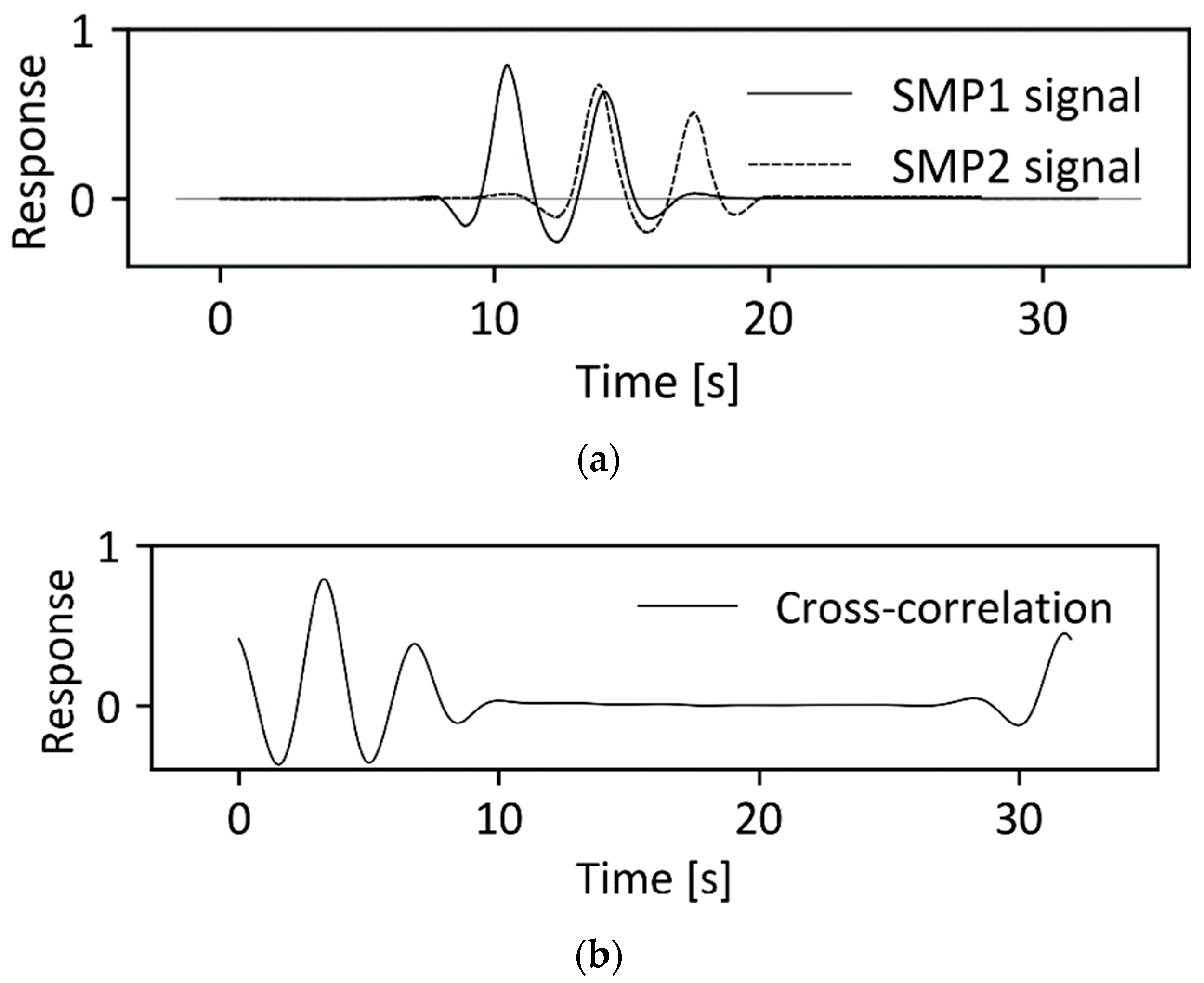
The correlation between two signals from SMPs defines the time shift of one signal relative to the other and hence is used to find the speed. An example for a one-carriage passenger train is presented in Figure 1. The solid and dashed traces of Figure 1a represent the signals measured at the first and the second SMP, respectively; Figure 1b shows the correlation. The location of the peak in the correlation is used to determine the time shift, 2.475 s in this case. The calculated time shift and the known distance between the SMPs are used to determine the speed of the vehicle.

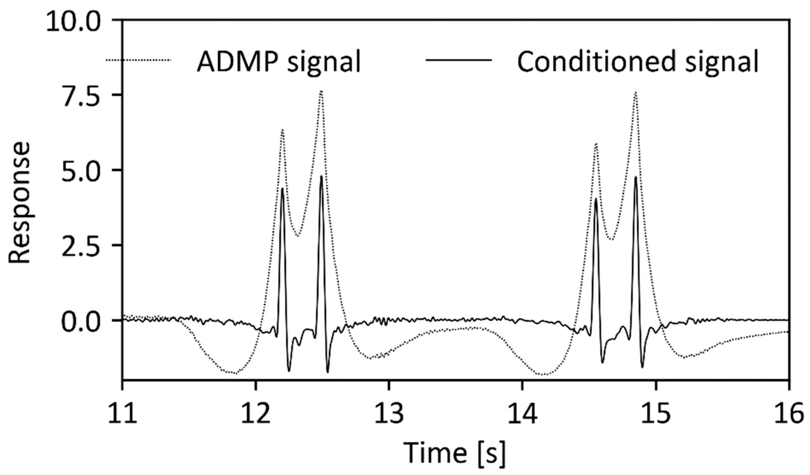
Once the vehicle speed is known, the axles of a train are detected using the same algorithm used for road bridges [33]. The signal from the sensor is conditioned by applying two moving average filters with different averaging lengths. The moving average with the shorter length is used to smooth out the high-frequency noise; the other is used to determine the general shape of the response. The two filtered signals are subtracted, and the resulting difference is examined to identify all peaks above a specified threshold level. These peaks correspond to the passing of individual axles. Figure 2 shows the axle detection signal and the conditioned signal for a one-carriage passenger train. The conditioned signals can be seen to have clear peaks corresponding to the four passing axles.

Once the speed of the vehicle and the times of passage of individual axles have been obtained, the intra- and inter-bogie spacings are calculated.

2.2. Influence Lines

Influence lines (IL) are key properties of a bridge, defining how it responds to loading at a given measurement point [24]. It has been shown that influence lines should be calculated directly from measurements [34] since theoretical influence lines rarely provide an accurate description of bridge behaviour. Two methods of “measuring” influence lines for bridges are known, the SiWIM approach [33] and the Matrix Method [35]. The Matrix Method uses vehicles of known axle loads and spacings and an inverse Moses algorithm to derive the experimental influence lines. This method is more straightforward and less time-consuming but requires vehicles of known weight, which are not always available at the time of setting-up the B-WIM system. More recently, a variation on this approach addresses the issue of requiring a vehicle of known weight [36].

The SiWIM system, used here, calculates the influence lines for the bridge using selected vehicles with unknown axle loads. Numerous evaluations of influence lines can be averaged to improve accuracy. Such ILs are normalised and require a scalar calibration factor to convert relative axle weights to actual weights (the C_F parameter in Equation (1)). A detailed explanation of this general procedure of IL calculation can be found in [33]. Briefly, the system models the IL with a cubic spline, chosen because its general characteristics match well with real influence lines—it is a curve of third order, continuous and smooth in first and second derivatives [32]. Some of the spline knots, representing supports and endpoints, are fixed, while some are allowed to vary. In order to determine the values and thus the shape of the IL, Equation (2) is used. Contrary to its use in weighing, where the only unknowns are axle loads, A_i, the function I(x) is unknown when calculating the IL. Since the system is no longer a linear function of all unknowns, Powell’s minimisation [32] is used to solve the problem.

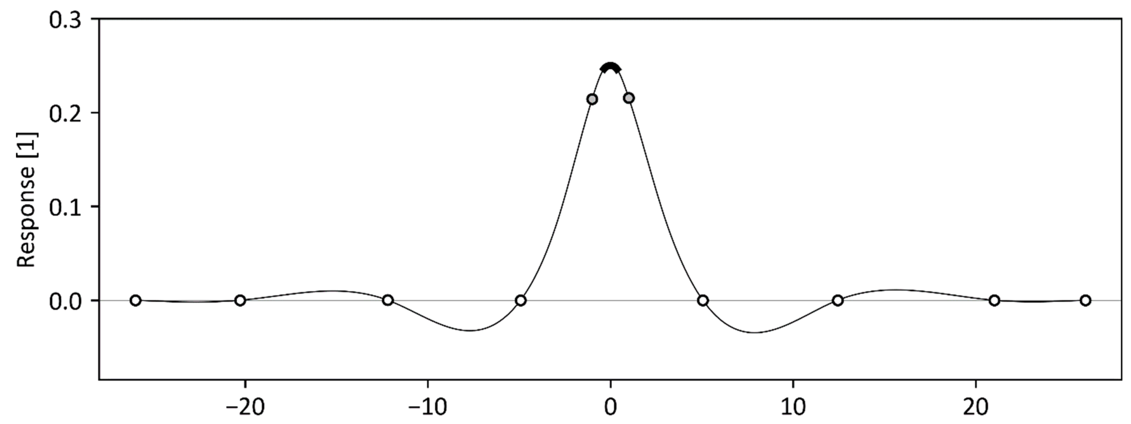
Figure 3 shows the IL calculated for the Nieporęt Bridge, for sensors mounted at the base of the truss at mid-span. The white points represent the fixed knots, while the ordinates of the two grey points were varied in order to obtain the best fit. For this bridge, local bending of the stringer beams dominated over global truss bending, making the influence line similar to that for a continuous beam with supports at truss chord locations. This effect was accentuated by setting the fixed knots to zero at the chord locations (Figure 3).

A theoretical influence line for an infinitely thin bridge (Euler Bernoulli beam) has a sharp peak at mid-span where the derivative is discontinuous. In contrast, the peak of the influence line for a real bridge has a rounded peak, which is approximated by a circular portion, whose radius corresponds roughly to the superstructure thickness. This peaked section is drawn in bold in Figure 3 and the radius was also varied to obtain the best fit.

3. RB-WIM Installation and Testing

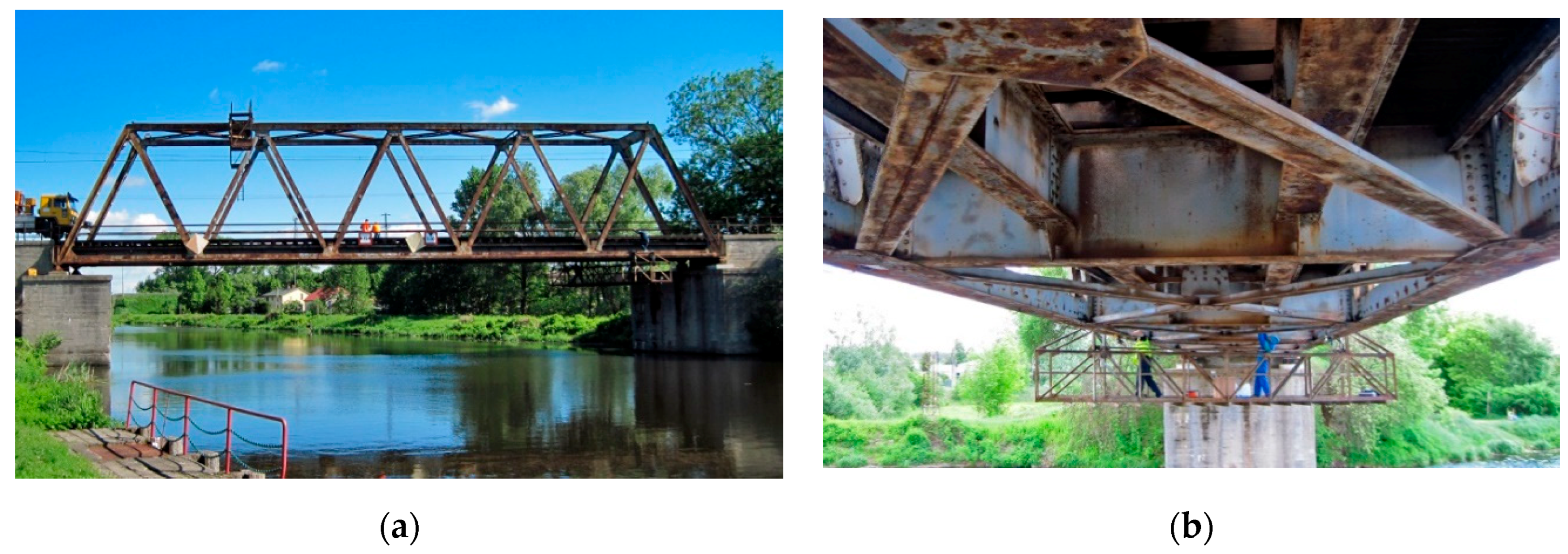
A single-track truss bridge in Poland was selected for testing of the RB-WIM system (Figure 4). The bridge is located in Nieporęt, near Warsaw. Constructed in the 1970s, it is one of over one thousand similar bridges in Poland [37]. It spans 40 m and consists of five 8 m long bays. The bridge has deteriorated significantly since first constructed. As a result, it does not carry heavy traffic load and the velocity of the crossing trains is limited to 20 km/h (considerably lower than the average train speed of 160 km/h in Poland) [38]. The speed restriction at the test bridge may raise a concern regarding the applicability of the study for higher traveling speeds. However, previous studies in road and railway B-WIM [26] have shown that there is no obvious correlation between accuracy and the speed of the vehicle. The application of the B-WIM system in weighting vehicles at full highway speed (checked against static weights) is demonstrated in several studies [25,39].

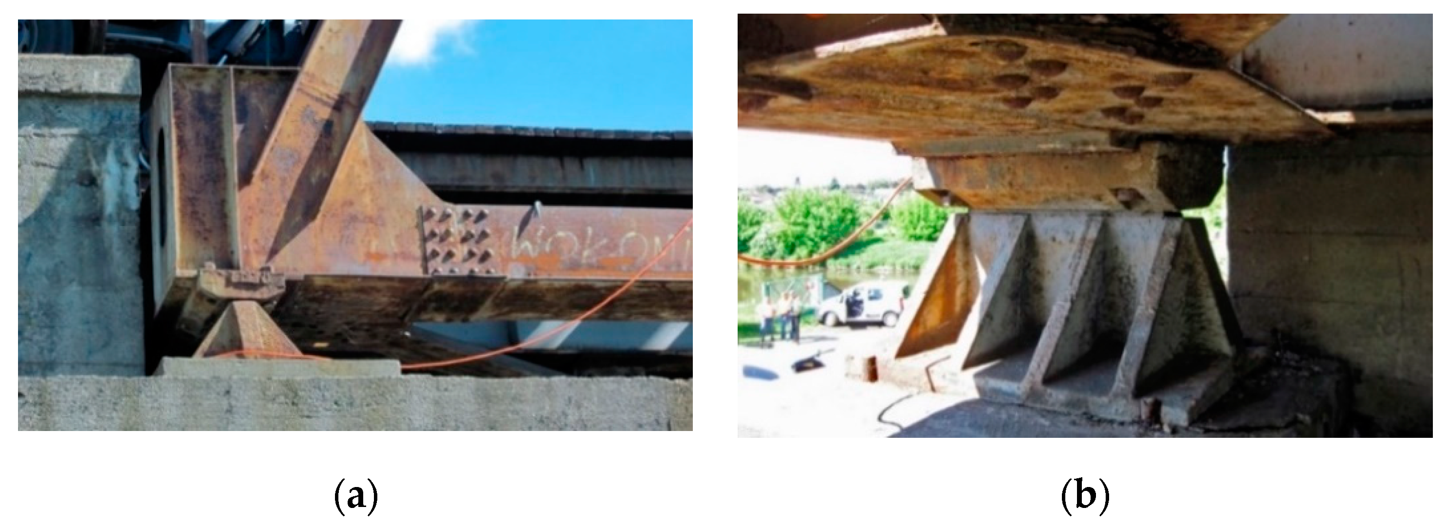
The bridge is supported on four steel bearings, illustrated in Figure 5, two at each end. It carries a single unballasted railway track that runs along the centre. The structure of the bridge consists of two main vertical trusses, one at either side. The trusses are connected along the bottom by six cross beams that are located at the node points of the bottom chord.

The railway track is supported by timber sleepers that span onto two “stringer” beams. These stringer beams extend longitudinally and are supported by the six cross beams. The loading on the track is transferred onto the sleepers and then onto the stringer beams. The stringer beams transfer the load into the cross beams, which are supported at the node points of the trusses.

The Nieporęt Bridge has been studied since mid-2007 due to interest from Polish Railways in the development of structural health monitoring (SHM) systems for railway bridges [40]. The bridge has been instrumented with a number of sensors, data from which are in the literature [40]. Prior to installation of the RB-WIM system, some of these published results were used to confirm the accuracy of the static model. For this purpose, a finite element model of the bridge was created using the Midas finite element software package. The bridge was modelled using beam elements, with full fixity assumed at node points. The design drawings were used to calculate cross sectional properties. A Young’s Modulus of E = 210 × 10⁶ kN/m² was assumed throughout [41]. 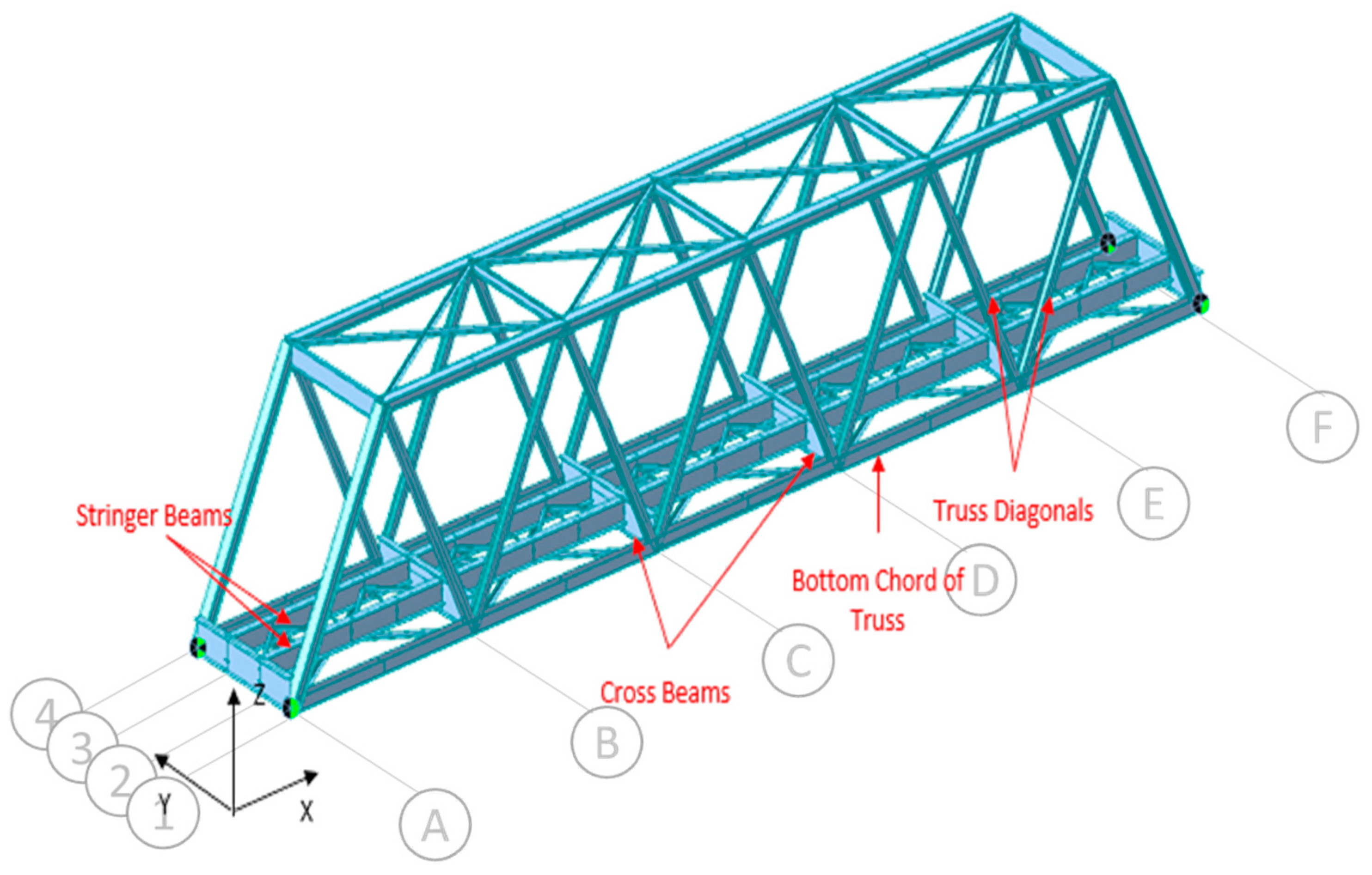Figure 6 shows the MIDAS model of the bridge, identifying some of the main structural elements. The rail and sleepers have been omitted for clarity. The numerical model of the bridge was validated at a number of important measurement locations using recordings from a previous measurement campaign [40]. Having established a good match between the response of the model and the measurements collected by Kołakowski et al. [40], it was used to develop the instrumentation strategy for the in-field testing of the RB-WIM concept.

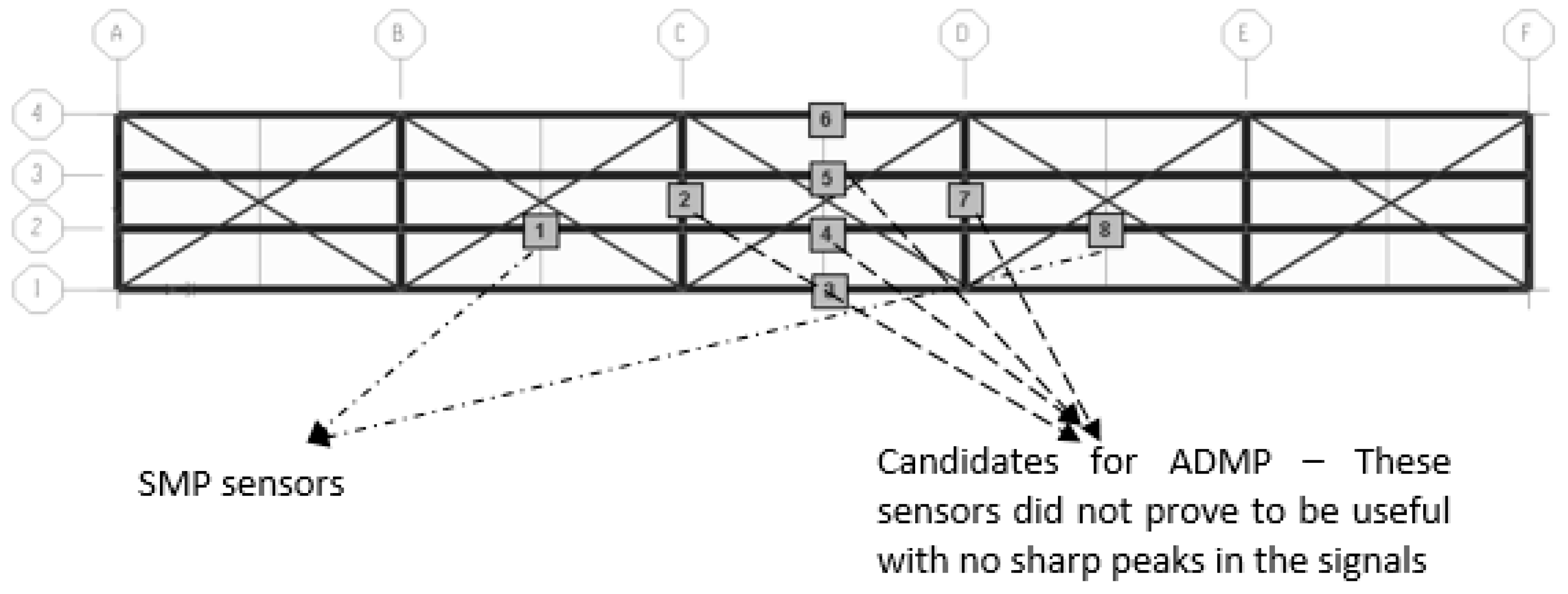
Strain transducers were installed on the longitudinal trusses, on the stringers, and on the cross beams to provide full coverage in the central part of the truss. Sensors were also located on one stringer beam in the bays on either side of the centre (i.e., sensors 1 and 8 shown in Figure 7). The locations of the sensors are marked with grey squares in Figure 7. The numbers represent the data acquisition channels. To avoid welding or drilling, steel mounting plates were used as interfaces. They were bonded to the structure with epoxy and, after hardening, the strain sensors were fastened with nuts. Additionally, strain gauges were bonded directly to the bridge at locations 3 through 6.

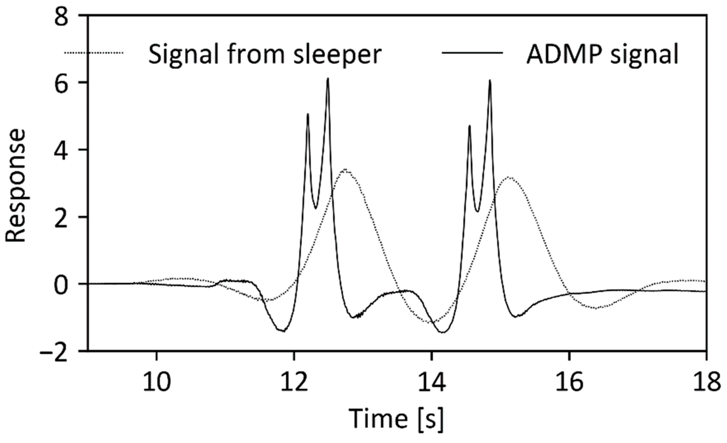
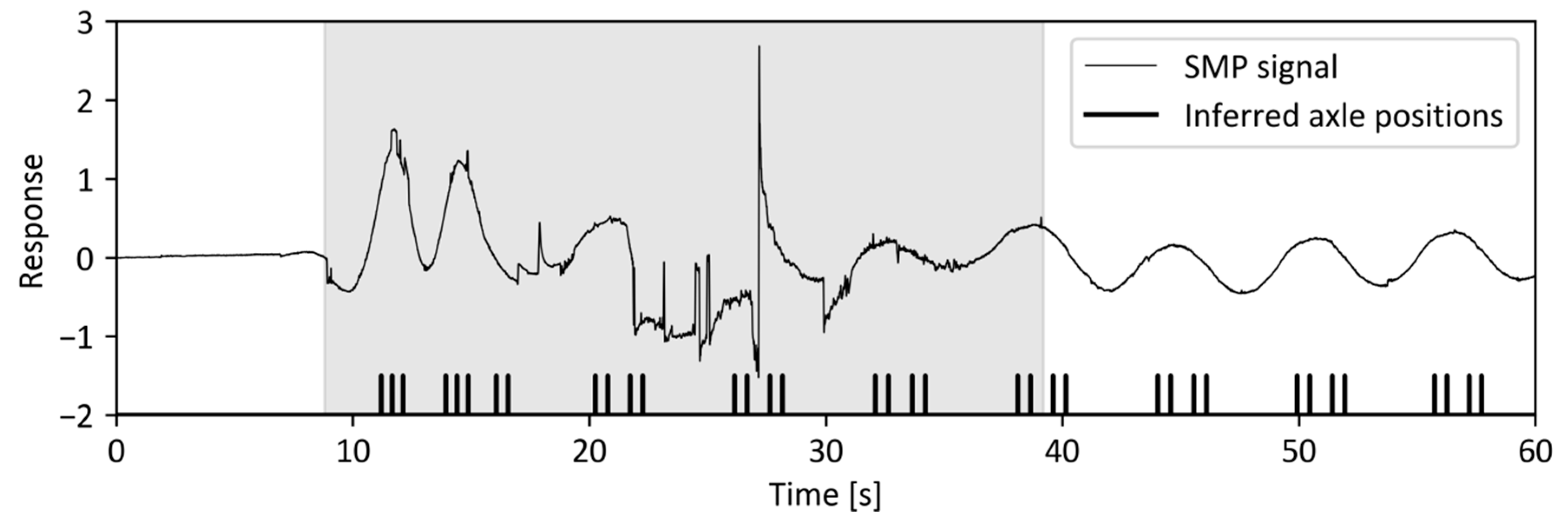
A desirable characteristic of a B-WIM installation is that any intervention on the track side is avoided, an important advantage from a safety and maintenance perspective. Therefore, it was envisaged that the sensors on the stringer beams, right under the sleepers, would be used for axle detection. However, signals from the passing trains revealed that the axle loads distributed over the entire rail-sleeper-bridge system did not provide sharp peaks to identify individual axles in a bogie (double or triple axles, Figure 8). Thus, the sensors were moved from their initial locations to the bottom flange of the rail between two sleepers.

Field testing was performed between 20th May and 25th May 2013. Over the first two days, the sensors and the system were installed. On 22nd May, the first of four calibration/test trains, which were weighed off-site, passed over the bridge. Signals from three other pre-weighed trains were also captured; two on 24th May and one on 25th May.

The four calibration/test trains were weighed on a low-speed weigh-in-motion scale in a railway yard in Warsaw that operates at speeds of up to 5 km/h. All of these trains consisted of a 6-axle locomotive and 25 to 38 carriages of different length, axle configuration, and loading. Due to the limitations of the low-speed device, only gross weights of carriages, without individual axle loads, were available for comparison with the B-WIM results.

4. Results and Discussion

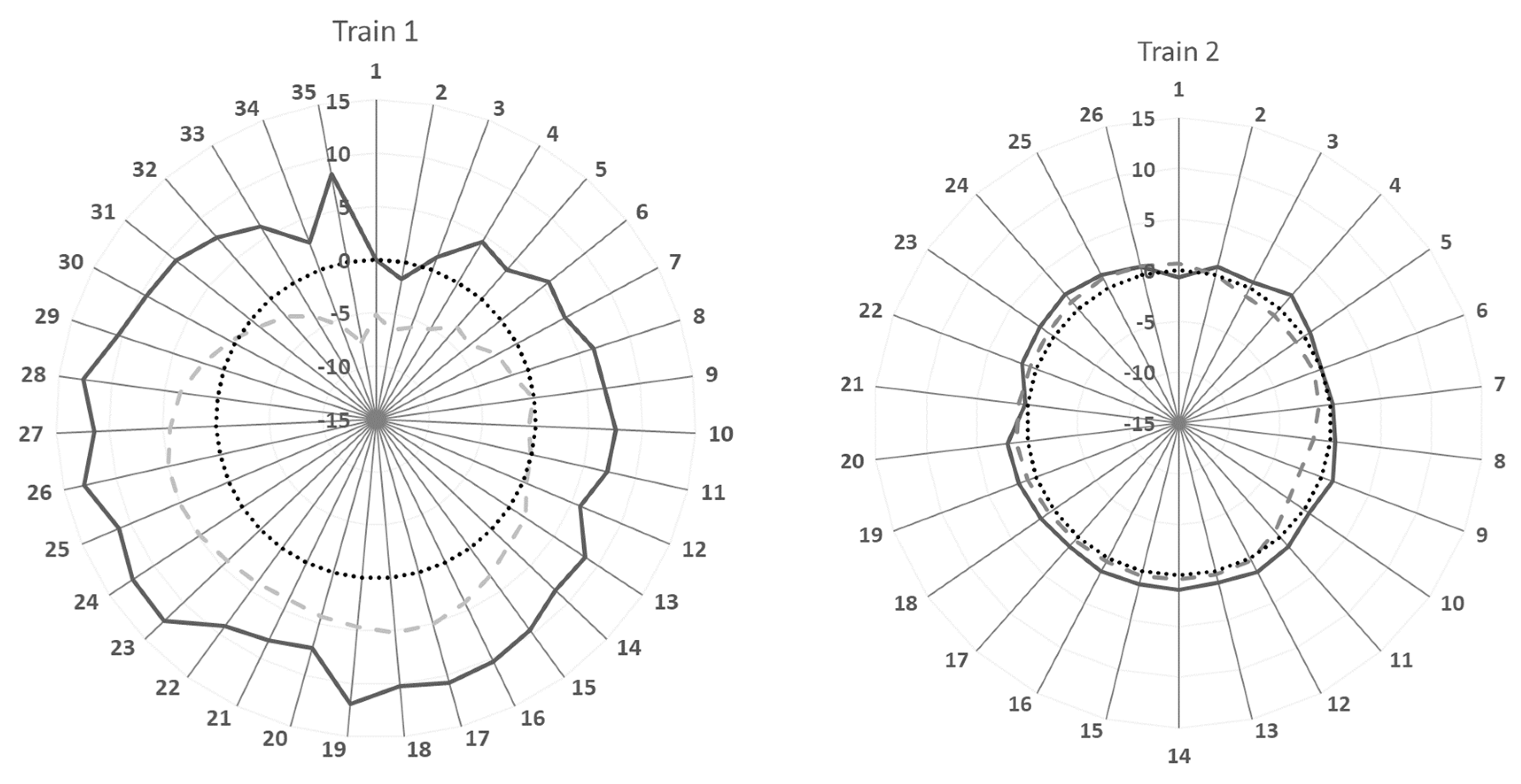
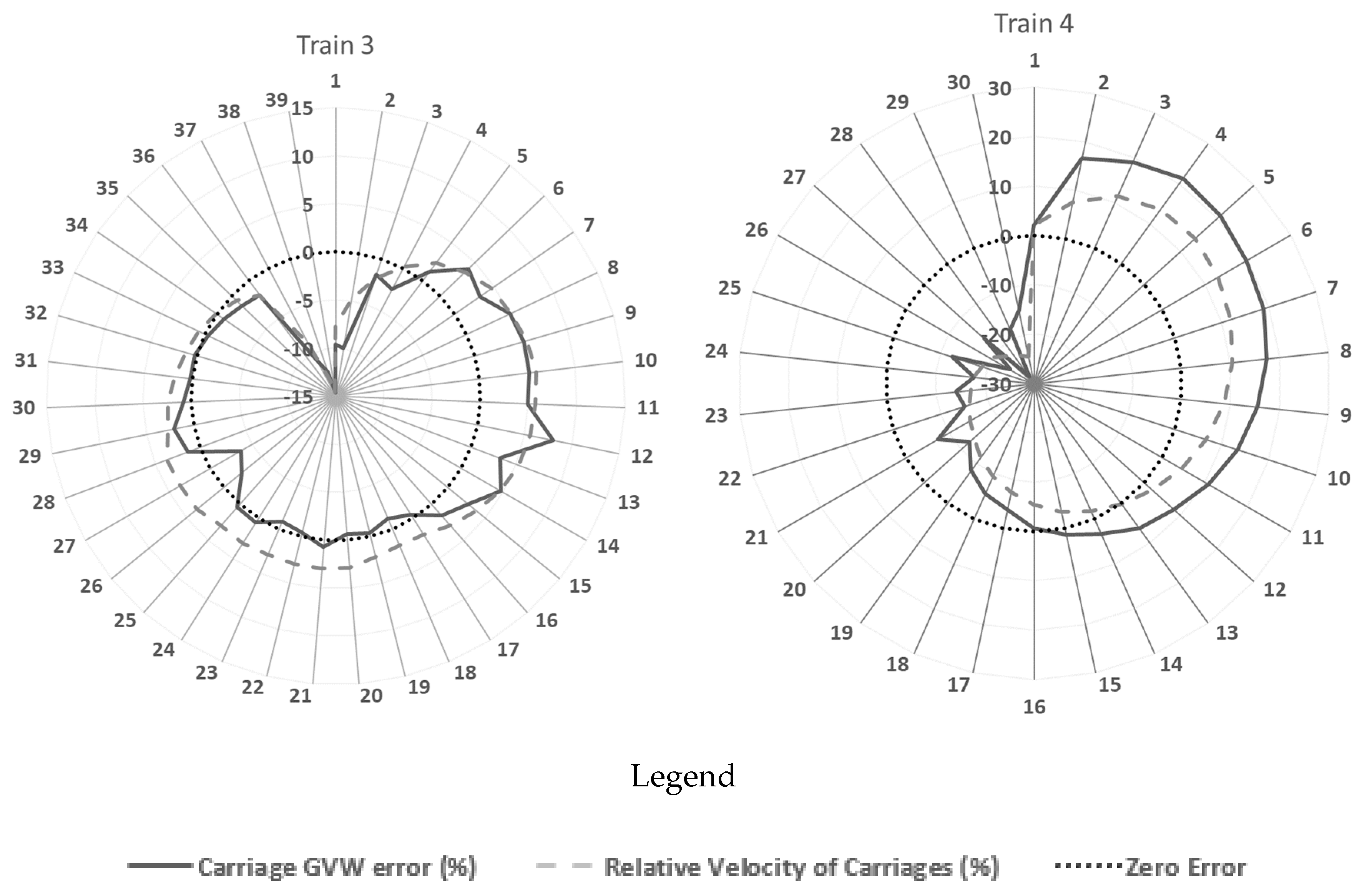
Figure 9 summarises the initial results for all four pre-weighed trains in a spider chart. The solid black line represents the error in GVW estimated using the RB-WIM algorithm applied to the 35 locomotives/individual carriages. The dashed grey line represents the relative velocity of individual carriages, calculated as the ratio of the individual carriage velocity to the average velocity of the entire train, as described in Section 2.1. While the train speed can be assumed to be constant at any point in time, it varies through time. The speed limit on the bridge was 20 km/h. It appears that this was not adhered to precisely by the drivers, but its presence resulted in significant braking and acceleration as the trains crossed.

It can be seen that the carriage accuracy for Train 2 represents the best match with maximum weight error of 2% and standard deviation of 0.64%. The maximum error in GVW estimation occurs in Train 4 with an error of up to 28%. The obvious reason for this error is the assumption of constant velocity for all carriages in an event where it is varying quite significantly about the mean. The assumption of constant velocity is reasonable on roads, as trucks typically cross a short-span bridge in one or two seconds, but trains are too long for such an assumption.

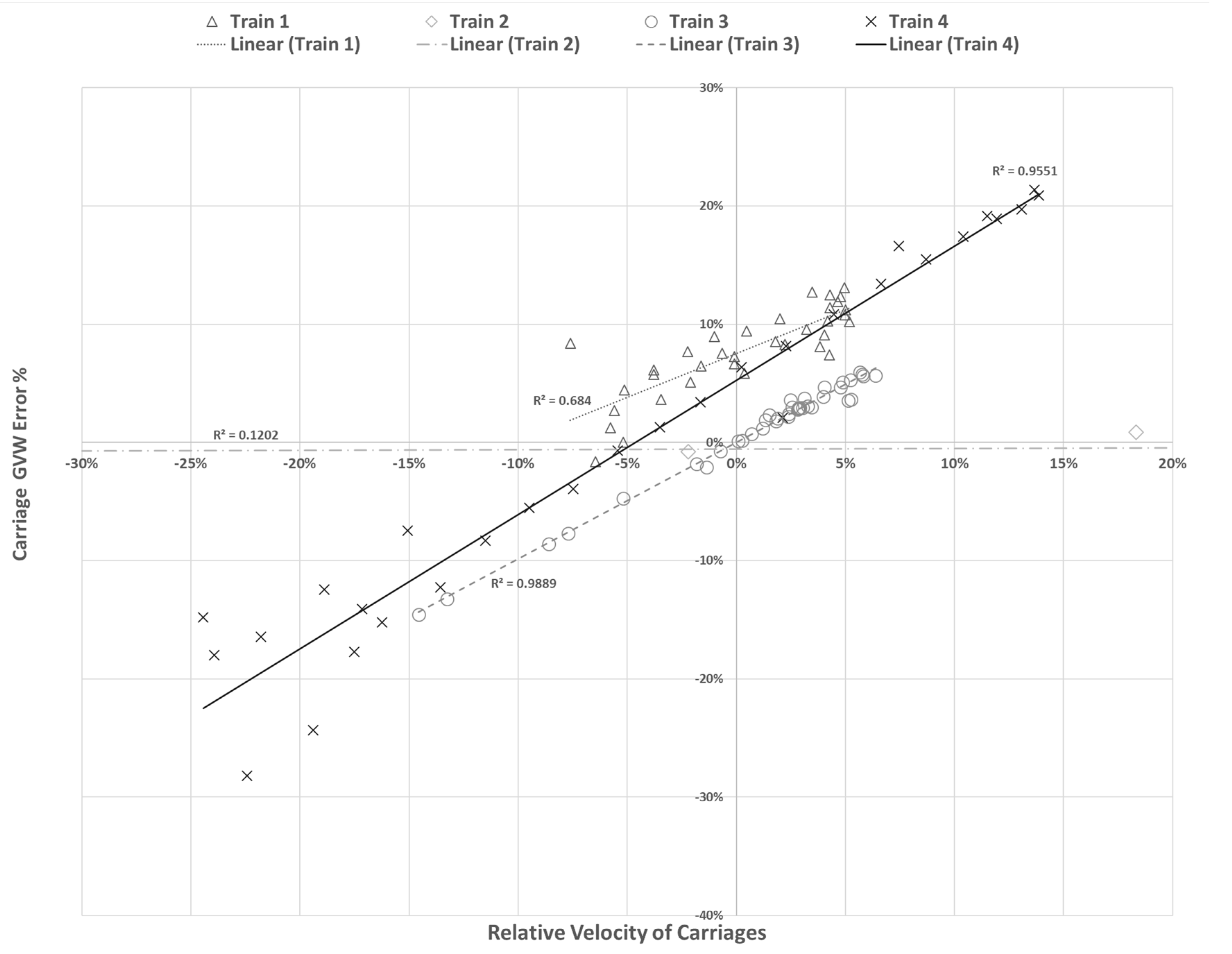
The speed variation was more pronounced for longer trains, some of which exceeded 500 m in length. As the variation in measured speed in the worst case (Train 4) surpassed 25% (negative error), the assumption of constant velocity clearly was not appropriate and had to be addressed. Figure 10 shows the correlation between the error in carriage GVW and the relative velocity for all carriages of all four trains. It can be seen that Trains 3 and 4 in particular show strong linear correlations between GVW error and relative velocity with correlation coefficients of 0.99 and 0.96, respectively.

To address this issue, the constant velocity of the whole train was replaced with different velocities for individual carriages. The additional step in the modified algorithm consists of determining the sections of the SMP signals where a locomotive/carriage is on the bridge (as isolated as possible), calculating the correlations for only those parts of the signals and assigning the resulting speeds to the locomotive/carriage in question.

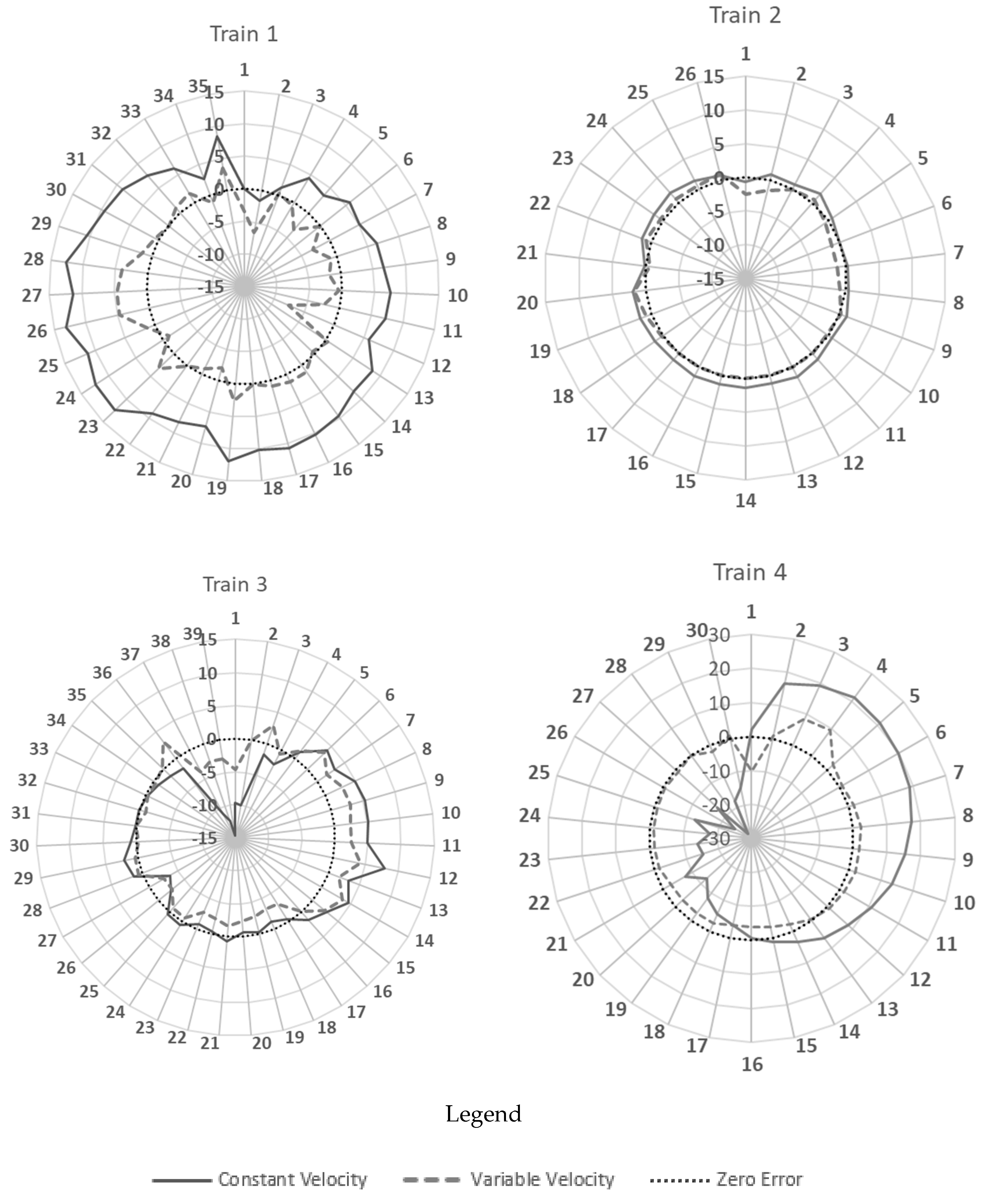
Figure 11 displays the errors in the predicted carriage gross weights for each train when considering (i) the average velocity of the train obtained from the entire train crossing (solid black line curves as shown in Figure 9) and (ii) variable velocities calculated for each carriage (dashed grey line). There are clear improvements in accuracy for all four trains. The improvements are less pronounced for Trains 2 and 3 but the accuracy for these was already good, and it is significant that where there were some larger errors in Train 3 (Carriages 37–39), these were greatly reduced. The improvements in Train 4 were quite pronounced although some errors persisted at Carriages 1, 3, and 4. This may be explained by the occurrence of heavy rain just before the crossing of this train and insufficient protection of the strain gauges (due to the short testing campaign), which resulted in a noisy speed measurement signal (the shaded area in Figure 12) and, consequently, unreliable velocity measurements for these carriages. Such errors can easily be avoided in the future by protecting the sensors against environmental effects.

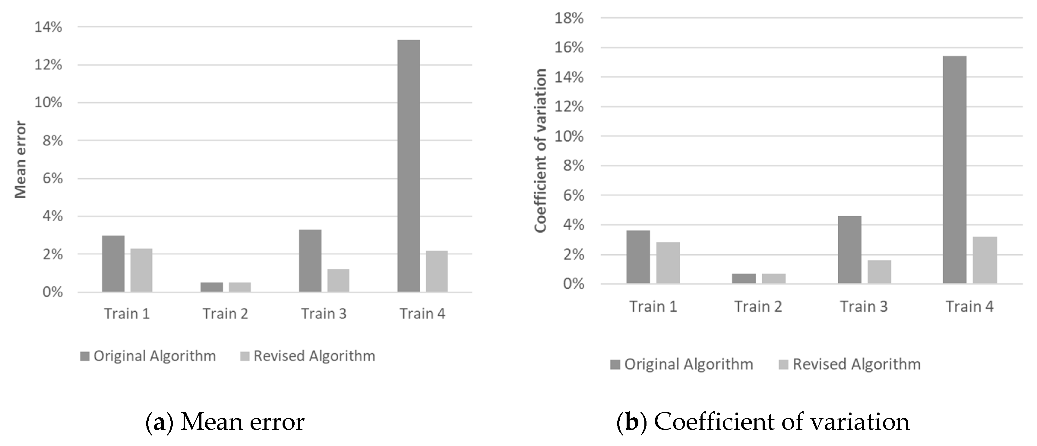
Figure 13 summarises the results obtained with the original RB-WIM algorithm and those obtained using the revised algorithm for all four reference trains (calibration trains). It can be seen from this figure that the mean error in GVW was considerably reduced by the revised algorithm. For Train 4 in particular, the maximum error was reduced from 28.19 to 10.17%. The weights of the Train 2 carriages were predicted very accurately, which can be linked to constant travelling speed and uniform distribution of carriage weights.

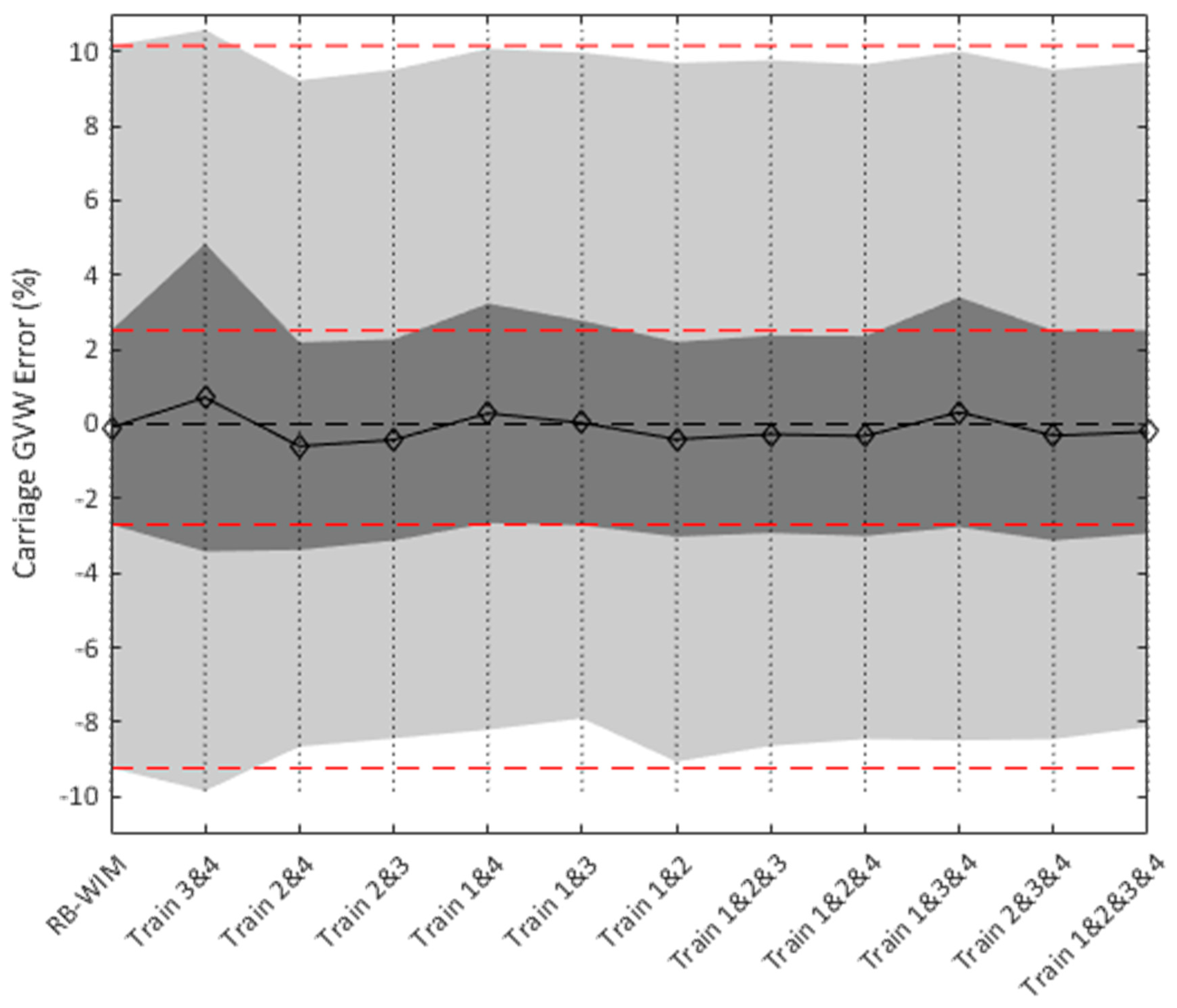
In the results up to this point, all four trains were used to calibrate the system. As such, the mean weight is not an indication of the accuracy, but the low standard deviation indicates an excellent level of accuracy relative to conventional road weigh-in-motion technologies. To investigate the sensitivity of the algorithm to the chosen calibration/test trains, 11 permutations of the calibration database were considered using all possible combinations of the four trains for calibration. These combinations were then used to produce a linear regression model between predicted GVW using the revised RB-WIM algorithm and the measured GVWs of carriages. Using each regression model, the GVWs of carriages and locomotives for each train were calculated and compared to the corresponding static values (Figure 14). The light grey area in this figure shows the minimum and maximum range of errors for each regression model and the dark grey represents the mean of the errors in carriage GVW ± one standard deviation (for each model). The horizontal dashed lines represent the minimum, maximum, and mean ± one standard deviation. It can be seen that there was little difference in the results except for calibration using Trains 3 and 4, likely due to the poor accuracy of Train 4.

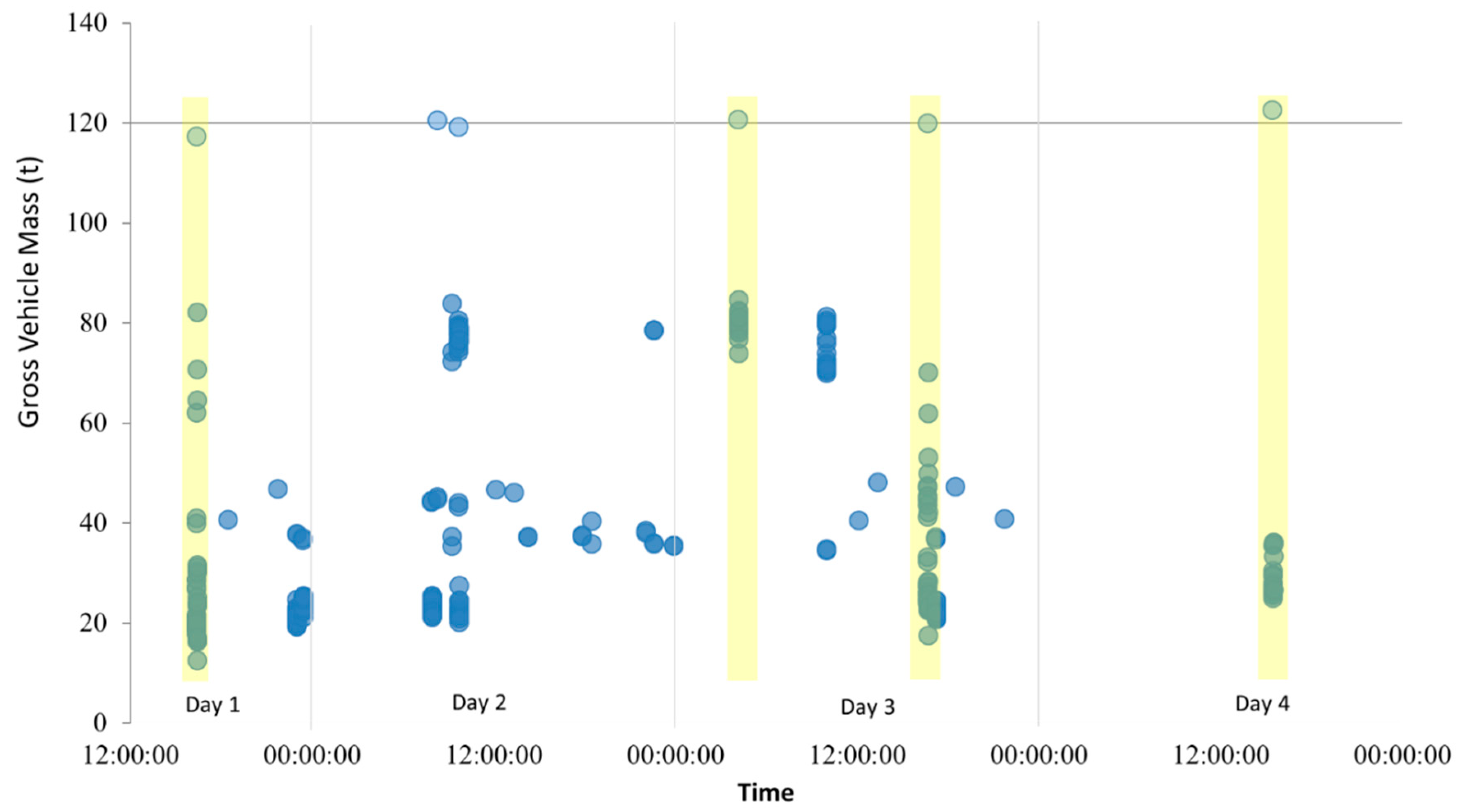
According to the railway authorities in Poland, there is a very common 120 t locomotive that operates on the network. At the time of the measurements for this study, in addition to the four calibration trains, another two trains with locomotives of approximate 120 t gross vehicle mass were measured. In this figure, each point represents an individual locomotive/carriage and points aligned in the vertical direction (with small timestamp difference) represent one train. Figure 15 presents all measured trains and time of measurement. Both in the trains with 120 t locomotives and the others, there were carriages/locomotives weighing about 80 t with most of the remaining carriages ranging between 20 t and 50 t.

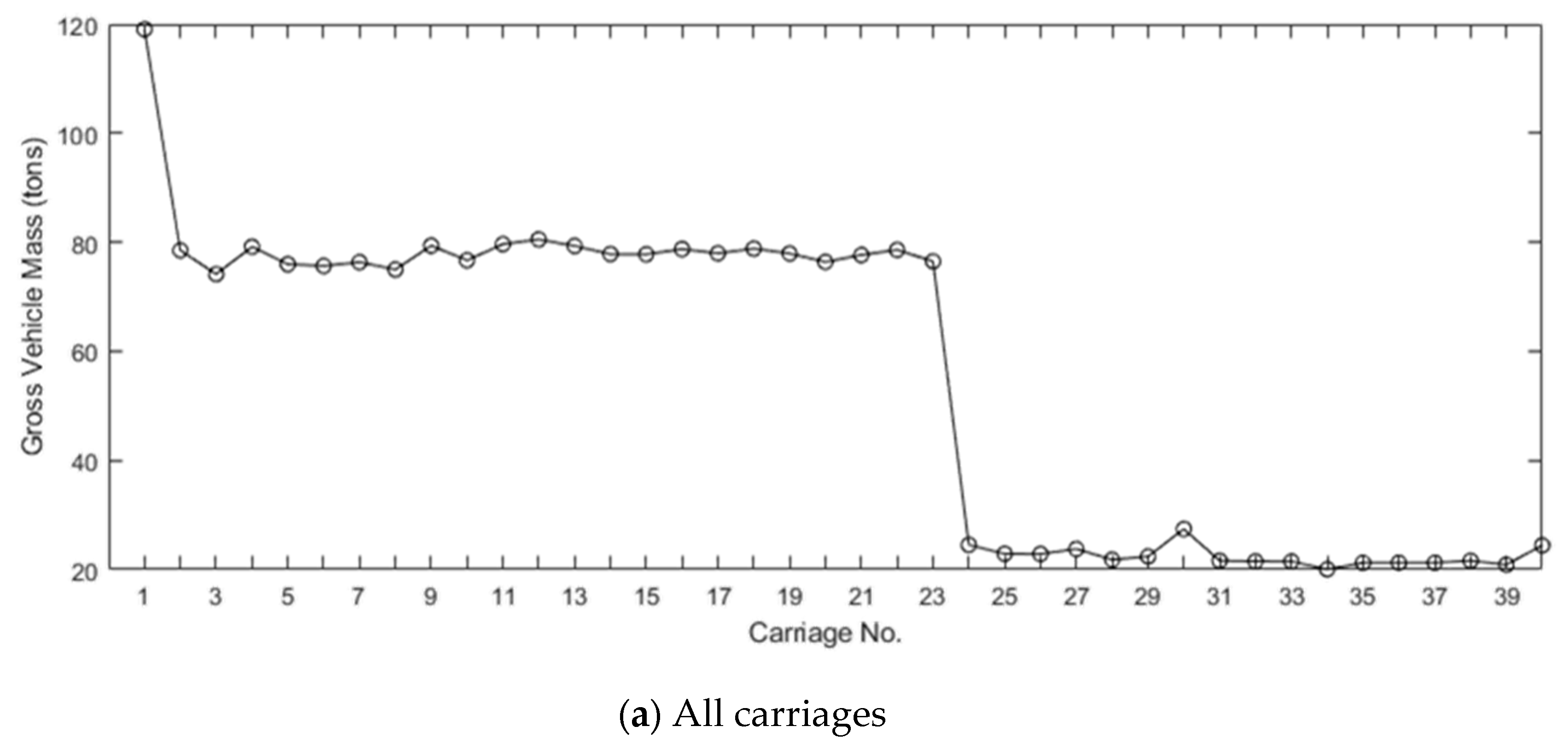
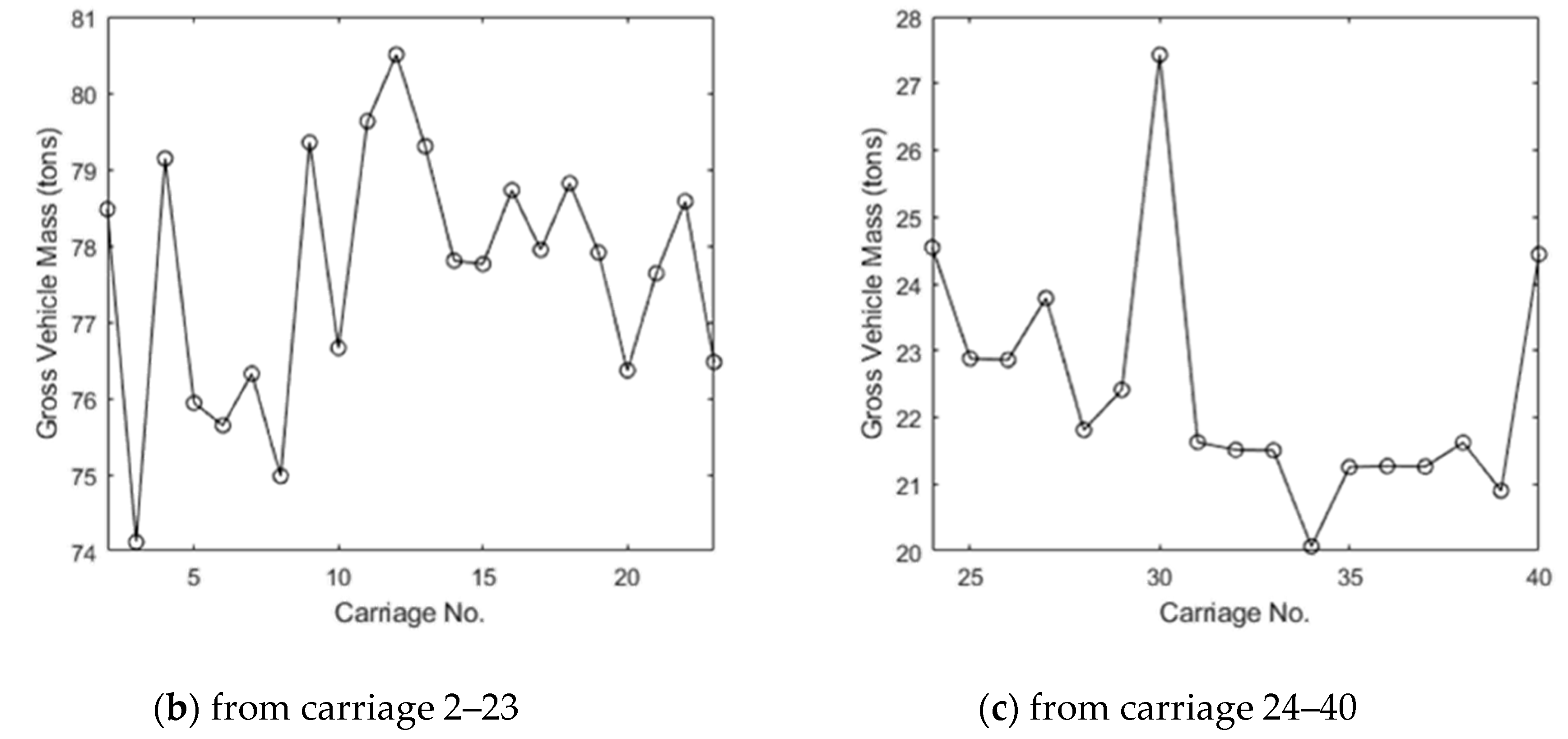
Figure 16a illustrates a particular train with 40 carriages, where it can be seen that the front carriages were much more heavily loaded than the others. Figure 16b,c provide a closer view of two groups of carriages 2–23 and carriages 24–40, respectively. Apart from the locomotive, the front carriages all had weights between 74 and 81 t. There was a dramatic drop at Carriage 24 and all remaining carriages weighed between 20 t and 28 t.

5. Conclusions

Knowing the true weights of trains is becoming more important, particularly in Europe, due to the splitting of the operation and infrastructure maintenance roles of the relevant authorities. This paper adapted a commercial road B-WIM system for use on railways. An old railway bridge in Nieporęt in Poland was used to test the accuracy of the new RB-WIM system.

Initial results demonstrated that one of four pre-weighed trains, the only one that crossed the bridge at constant speed, was weighed very accurately, with all carriage weight errors falling within the −0.9% to 1.6% error interval. Disappointing levels of accuracy for the other pre-weighed trains was shown to be the result of variable carriage speed in the time that the train took to cross the bridge. Results improved significantly when this was addressed, with 75% of all calculated carriage weights falling within ±2% and 97% of them falling within ±5% of their actual values. These values include 4 carriages that had an issue with axle detection due to rain.

In summary, the study has shown that the common assumption of constant velocity in bridge-WIM theory is not appropriate for trains. Due to the length of a train, the change in velocity can be considerable and neglecting this change can lead to significant errors in bridge-WIM algorithms. In the case of the selected bridge, this issue is of particular importance due to the speed restriction in place and continuous braking and acceleration. It should be noted that higher traveling speed and track irregularities may have an impact on the accuracy of the algorithm; however, these factors were not investigated in this study.