Article

The Elastic Wave Propagation in Rectangular Waveguide Structure: Determination of Dispersion Curves and Their Application in Nondestructive Techniques

by
Eduardo Becker Groth
1,
Thomas Gabriel Rosauro Clarke
1,
Guilherme Schumacher da Silva
2,
Ignacio Iturrioz
2,* and
Giuseppe Lacidogna
3
1
Physical Metallurgy Laboratory, LAMEF, Engineering School, Federal University of Rio Grande do Sul, Porto Alegre 91509-900, Brazil
2
Applied Mechanical Group, GMAP, Engineering School, Universidade Federal do Rio Grande do Sul, Porto Alegre 90050-170, Brazil
3
Politecnico di Torino, Department of Structural, Geotechnical and Building Engineering, 10129 Torino, Italy
*
Author to whom correspondence should be addressed.
Appl. Sci. 2020, 10(12), 4401; https://doi.org/10.3390/app10124401
Submission received: 30 May 2020 / Revised: 16 June 2020 / Accepted: 18 June 2020 / Published: 26 June 2020
(This article belongs to the Special Issue Nondestructive Testing (NDT): Volume II)

Abstract

:
The use of mechanic waves for assessing structural integrity is a well-known non-destructive technique (NDT). The ultrasound applied in the guided wave in particular requires significant effort in order to understand the complexities of the propagation so as to develop new methods in damage detection, in this case, knowing the interaction between the wave propagation and the geometry of the waveguides is mandatory. In the present work, the wave propagation in rectangular steel rod is presented. In this study, the section dimensions were fixed as 5 × 15 [mm], a typical element of the flexible riser structural amour commonly used in the offshore oil industry. The studies here presented were restricted to [0, 100 KHz] frequencies. This frequency interval is in the range of commercial waveguide equipment commonly applied in ducts in NDT applications. The computation of the dispersion curves is performed by using three different methodologies: (i) analytical solutions, (ii) a method that combines analytical approaches with finite element methods (SAFE), and (iii) experimental method that extracted information from the rod using laser vibrometers and piezoelectric actuators. Finally, two applications based on the dispersion curves determined in the rectangular waveguide are presented to illustrate the possibilities of the curve dispersion knowledge related to the specific geometry in the development and application linked to NDT. The first application consists on showing the possibilities of the techniques that use a fiber grating Bragg cell (FGB) to measure the wave displacement and the second application involves the simulation of pre-fissured prismatic waveguide aimed at searching to induce three characteristic acoustic events. The model was built combining the finite element method and a version of the discrete element method.

1. Introduction

Techniques based on elastic wave propagation are commonly used in engineering to detect damage and to control structures such as pressure vessel, piping, among others. The study of wave propagation in solids has been a source of inspiration for nondestructive techniques, not only to develop them but also to monitor the structural assessment (SHM).
The prismatic bar could be considered simplified components of a flexible pipe (riser) used commonly in the offshore oil industry, more specifically when forming the structural amour layer of this system (see Figure 1a). The original motivation of the present work consists on developing an non-destructive technique (NDT) using a wave propagation framework that allows detecting damage in a critical region of the riser close to the platform connection (see Figure 1b). Details about the application of the NDT based on guided waves in this kind of structure can be seen [1,2].
The advance of NDT has increasingly allowed the service failures prediction, consequently reducing the maintenance cost and raising the structure reliability throughout its useful life [3,4,5]. The NDT can be divided into active and passive methods. In the case of active methods, the structure is excited with a perturbation that propagates interacting with defects, thus, enabling the structural integrity assessment. In the passive techniques, a typical an example is the acoustic emission technique (AE) where the excitation is produced when the damage advances due to an overload or when being submitted to conditions of utilization. This excitation is called event, and the analysis of the wave propagation emitted by the source of emission allows us to obtain information not only about the defect but also the conditions of its growth and, thus, carry out the structure health monitoring (SHM) [3,4,5].
In both techniques, the condition of the information extracted from the tests, regarding the wave propagation properties (inherent of the structure geometry and material) influence the data extracted. In this context, the present work was developed with the main objective of presenting in detail the propagation of elastic waves in rectangular isotropic steel rod of 15 × 5 [mm] where the attenuation due to the material viscosity is neglected [6]. The approach aimed at studying the wave propagation in this geometry lets us advance in our main goal to develop the NDE system to identify the type of damage in the problem described above and illustrated in Figure 1b. In the present study, the frequency range of interest is [0, 100 kHz], this frequency interval is within the range of wave-guided commercial equipment commonly applied in ducts in NDT applications. The attenuation due to the energy dissipation is proportional to the square of the frequency of the excitation. This fact influences the definition of the frequency range of work.
Within the elastic wave propagation fields, there are the guided waves (GW), present in slender structures, where one or two geometric dimensions are smaller than the others (waveguide). Examples of this type of structure are ducts, train rails, and plates. GW-based experiments have changed the nondestructive techniques drastically because they allow the evaluation of large areas from point transducers [6]. Knowing the propagation modes in the waveguides is fundamental to the success of the NDT based on GW.
The dispersion curves of the cited structure allow us to build by using the analytical and semi-analytical methods. The rod dispersion curves are also computed using experimental results. The comparison between the different methodologies used not only let verified the limitation and vantages of the method used but also understand how the waves travel in this kind of elements.
Two examples were present to illustrate the curve dispersion applications: (i) The wave displacement detection using the fiber grating Bragg (FGB) technique was applied to show this not conventional technique in the present context and (ii) the simulation of a rectangular waveguide with a pre-fissure is loaded to induce characteristic acoustic emission events shows how the dispersion curves knowledge could to improve to understand the characteristics of the signal emitted from the source and also the potential possibilities to use a non-conventional model that combines the finite element method and a version of the discrete element method in this context.

2. Propagation on Stems with Rectangular Section

In solid media, there are two basic ways of propagating energy: one associated with the compression and the medium rarefaction and other related to the shear movements between the perpendicular planes to the propagated direction [5]. From these two types of propagation two kinds of waves emerge in infinite solid media: the P (dilatational) and S (equivoluminial) waves. The P and S waves have a velocity propagation c p = ( λ + 2 μ ) / ρ and c s = μ / ρ , respectively, where λ′ and μ are the Lamé constants [Pa] and ρ is the density of the medium [ k g / m 3 ] . When the P and S waves find the solid interface, part of the incident wave refracted out and the other part of it is reflected into the body.
The relationship between the amplitudes of refracted and reflected waves depends on the elastic properties and the density of the interface media, as well as the refraction and reflection angles of the reflected waves which are governed by the Snell’s law [7,8,9]. If the propagation medium (body) has one or two finite dimensions, it is called a waveguide. The P and S waves that propagate in waveguides interact with the guide boundaries and generate patterns of energy propagation known as modes [6,8]. The propagation modes, also called modal waves, depend not only on the material properties but also on its geometry.
Every structure considered as waveguide has its propagation characteristics, and the rectangular section has been widely investigated, among other works, it is possible to cite [8,10,11,12,13]. Following the theoretical basis model of wave propagation in rectangular rods is presented.

2.1. Analytical Models of Wave Propagation in Waveguides

Lamb [14], in 1917, developed a solution for wave propagation in plates whose response relates to angular frequency (ω) with the wavelength (λ). This solution is known as the transcendental equations of Rayleigh–Lamb [6,8]. In addition to the analytical solution, the graphical representation of these equations is known as the plate dispersion curves. In the dispersion curves, each curve represents a propagation mode [15], which can be written in terms either of frequency (ω = 2π/T, f = 1/T) vs. the wavenumber (k = 2π/λ k = 1/λ), or phase velocity (c) vs. frequency, remembering that c = ω/k. Moreover, it is possible to represent the dispersion curves in terms of group velocity vs. frequency since the group velocity is defined as: c g = d ω / dk [6]. This way to present the solution of the waveguide propagation (curves that represent the propagation modes and their frequency and wavenumber relations) is usual in acoustics, acting as a map of the waveguide propagation. There are a lot of publications on the computational methods on which research was based on to build the dispersion curves; among others, we cited the work presented in [16] where the key works in this topic are commented.
In the particular case of a rectangular waveguide the dispersion curves obtained using an analytical approach presents two options: to consider the waveguide as a plate or as a beam, both with an “infinite” length. Next, the most relevant computational methods due to their historical relevance and for their practicality are presented:
Considering the rectangular rod as a plate, Mindlin and Fox [10] developed an adaptation of the Lamb plate theory applied to rectangular sections. Mode wave families propagating on plates are called: Sn (symmetrical to the plate), An (antisymmetric) and SHn (horizontal shear, perpendicular to the propagation direction). In Auld [8], an analogous model is presented, where two fundamental modes, S0 and A0 are defined by the expressions ω = kcs and ω = kcp. The family modes Sn and An tend to these fundamental modes when the frequencies decrease. In Figure 2 the modes Sn and An are presented for the rectangular rod studied and modes A0 and S0 are highlighted.
If the rectangular rod is considered as a beam, it is possible to generate the dispersion curves from the balance of forces applied over an infinitesimal portion of the waveguide, and considering the hypotheses that allow the solution of the differential equation of equilibrium in terms of ω and k [11,17]. In Figure 3, four modes from three known movements of beams: axial tension, torsion, and bending in two main directions are shown. In Table 1, the expression that defines these curves are presented and described.
The expressions above (Table 1) present the dispersion function of each mode, where ρ is the density, C t the modulus of torsional stiffness, J the polar moment of inertia, A the transversal area, I the moment of inertia with respect to the bending axis (Axis 2 or 3, depicted in Figure 5b) and E the axial elastic modulus.
Some corrections can be applied to the analytical expressions obtained to represent the dispersion curves either for the formulations from the plate or beam model. For example: Love correction for longitudinal waves in beams [11]; modification of the dispersion relation for the longitudinal waves based on Lamb’s formulation applied in Plates presented by Morse [12]; Timoshenko’s correction in the transverse waves of the beam model [18]. In all cases, the corrections are made aiming to improve the analytical solutions.
Notice that the curves S0 presented in Figure 4 coincide with the longitudinal curve presented in Figure 3, and the A0 mode of the Figure 4 is the asymptote of the flexural 3 curve presented in Figure 3.
Cegla [13] presents an alternative way to compute the rectangular rod dispersion curves using the Rayleigh-Lamb equations. The curves were obtained by solving the Rayleigh–Lamb equations by the software Disperse [19], and are presented in Figure 3, using the beam section aforementioned in this work. Notice that the plate overlapping technique proposed by Cegla [13] is not able to compute the torsional wave modes.

2.2. Semi-Analytical Models to Build the Dispersion Curves

The semi-analytical finite element method (SAFE) is a technique that uses finite element analysis (FEM) for the dispersion curves confection of a given waveguide. They are called semi-analytic because these models require an analytical condition that by-pass the fact that the waveguide has at least one “infinite” dimension. The analytical condition allows relating the frequency with the wave number.
This method allows building the dispersion curves of complex geometry waveguides, such as train rails [20], stem or plates composed by two or more materials [21], among a series of other possibilities. The central idea of this technique is to compute the natural vibration frequencies of models that incorporate, using an analytical restriction, the infinite dimensions of the waveguide. As mentioned in [22], the first SAFE method appear in 1973 with Lagasse [23], who developed a procedure for working with waveguides of complex geometry with one face clamped, and with Aalami [24] that developed a method to compute dispersion curves for orthotropic rectangular waveguides.
Since these pioneer works, SAFE methods have been constantly evolving and making progress. A proof of this fact is the great number of works in the scientific community, among others could be cited: [25], where the study of 3D finite element model combined with periodic boundary conditions in the infinite direction is implemented to compute the dispersion curves; [26], the study where the focus is to build the dispersion curves in anisotropic waveguides; [27], the study where the dispersion curves are applied in the context of nonlinear wave propagation; [28], the study where the dispersion curves are computed using the COMSOL/FEM package; [29], where the dispersion curves are implemented considering an harmonic function in the infinite dimension, [30], where the dispersion curves is used as tool in the area of geophysics; and finally [31,32], where the dispersion curves are used in order to understand the wave propagation in textile composite with complex microstructure.
In the present paper, two SAFE methods, Pedroi et al. [28] and Sorohan et al. [25] are used to make the dispersion curves of a waveguide with rectangular section (15 × 5 [mm]), E = 205 GPa and ν = 0.29. Next, the theoretical framework of both methodologies and the results for the rectangular rod studied are presented.
SAFE, proposed by Pedroi et al. [28]: In this method the displacement field in the infinite direction (1) according to Figure 5g, occurs through the imposition of the displacement field presented in Equation (1), on the problem described in Equations (2) and (3).
u = U ( x 2 , x 3 ) e 1 ( kx 1 ω t )
where u represents the displacement vector, k the wavenumber, ω the frequency, x the spatial coordinate, t the time and U the amplitude of the displacement in the transverse direction of the waveguide. Equation (2) is the Cauchy equation, which governs the static equilibrium in a domain Ω and Equation (3) represents the stresses σ i on the contour Γ.
C ijkl 2 u j x k x l + ρ ω 2 u i = 0 em   Ω
σ i = C ijkl u j x l n k   em   Γ
where C is the elastic constitutive tensor and n k are the components of the normal versors with i, j, k and l = 1, 2, 3.
Substituting (1) into (2) and (3) yields the system of equations to be solved as a quadratic eigenvalue problem. It is possible to implement this method in commercial finite element software to solve generalized eigenvalue problem presented as follows:
λ ^   d a U ¯ + ( c U ¯ + α U ¯ ) β 1 U ¯ a U ¯ = f
The Equation (4) is implemented using the finite element method for its spatial discretization, in the environment of COMSOL [29]. Where d a   ,   c   ,   a ,   f ,   α ,   β 1 represents matrix coefficients that allow to adapt the generalized problem of eigenvalues to the problem associated with Equation (2). In addition, in Equation (4) λ represents the vector of eigenvalues, U ¯ a matrix with the eigenvectors associated with each eigenvalue and ∇ (.) the differential operator. In the contours of the problem the condition of Neumann is applied:
n ( c U ¯ + α U ¯ ) = 0
where “n” represents the normal versor at each point on the contour. Solving the problem for different values of ω, the eigenvalues found correspond to the wavenumbers associated with each frequency value ω. In this way, it is possible to assemble the dispersion curves with the specific guide wave geometry. The matrix coefficients used can be found in the appendix C of [33] and the complete implementation detail in [28]. Figure 5a shows the results obtained, in terms of the dispersion curves, Figure 5b–f shows the displacement field of each wave modes obtained in the solution of the differential equation. Finally, in Figure 5g, the waveguide scheme with the reference axes is indicated.
SAFE proposed by Sorohan et al. [25]: In the present case, a finite element model with three dimensions was used, presenting a portion of the waveguide length L with periodic boundary conditions applied under the end faces perpendicular to the propagating direction.
The implementation of periodic boundary condition consist of making at x = 0 displacement of the model-dependent to the displacement of the face at x = L. Figure 6 shows schematically what the FEM model represents in the waveguide that is being studied. With the 3D FEM model and boundary conditions implemented, a modal analysis was carried out, and the natural frequencies and modes associated were obtained. From the fields of displacements obtained, by visual inspection, the p-value is reached, i.e., the number of times that the mode configuration is repeated in the Model length L. The wavelength can be written as follows:
λ = L p .
The pair of frequencies and wave number (f, k) associated with each wave mode were identified manually scanning the frequency range of interest, FEM models with L of 0.5, 0.25, 0.1 and 0.005 [m] were used.
In Figure 7, the response obtained for the section of interest calculated using the software ANSYS [34] is presented. Details of the method implemented are found in Sorohan et al. [25].

3. Experimental Analyses

In the present section, experimental analyses of the elastic wave propagation in rectangular section waveguides are illustrated. The four fundamental modes will be excited; applying a tone burst force with main frequency bands between 10 to 100 kHz. As a response, the displacements were measured at equally distanced points arranged along the waveguide propagating direction. The information of every test was saved in a matrix ([s] × [m]), where the colons indicate the spatial point where the sensor was fixed and the rows indicate the information stored in each time.
Applying the double Fourier transform technique [35] in the data collected, the dispersion curve domain (frequency [1/s] × wave number [1/m]) was written. Consequently, it is possible to identify the wavelength and frequency of the wave propagating in the waveguide. It is possible to induce a particular space mode applying excitation forces in different directions, with a tone burst function as a temporal variation. As a result, the dispersion curves for a frequency-wave number dominium were obtained. The dispersion curves obtained with this methodology were compared with the dispersion curves obtained by the SAFE methods already presented in [33]. Preliminary, experimental and theoretical results also were presented by the authors in [36].
The setup consists of:
-
A bar, made of ABNT 1020 steel [37], with dimensions of 5 × 15 × 1500 [mm] used as waveguide.
-
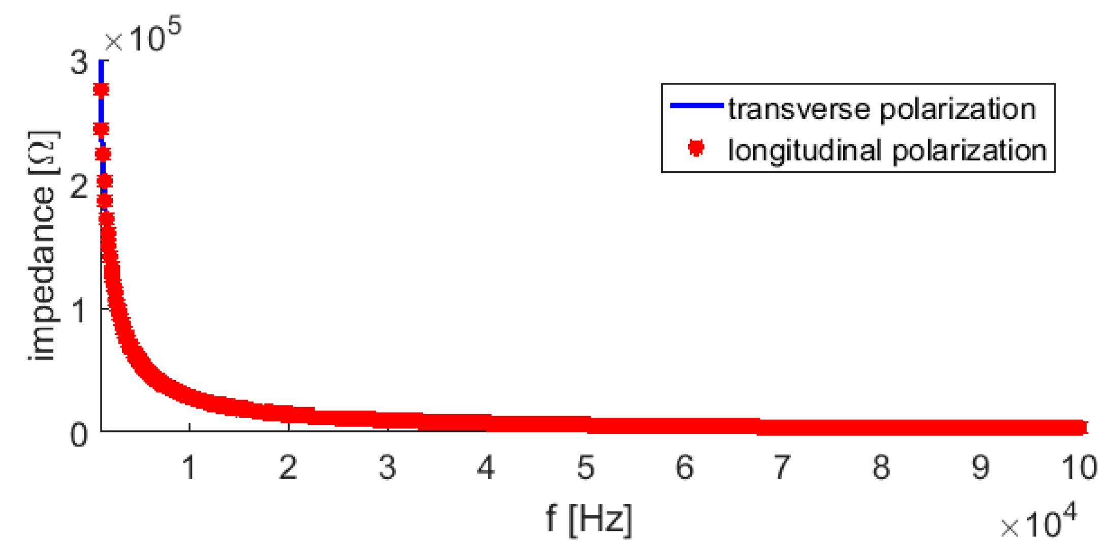
Two piezoelectric ceramics (PZT) Ferroperm®, with dimensions 1 × 3 × 13 [mm] and longitudinal and perpendicular polarizations which were used as an excitation transducer. Its frequency vs. Impedance response is presented in Figure 8, where it is possible to perceive that in the interval of frequency used [0, 100 KHz], these transductors present a response without resonances for the longitudinal and transversal polarization.
-
A function generator Agilient (Keysight) 33,521, used to create an excitation signal that applies a potential difference to the piezoelectric ceramics transducer; a voltage amplifier Krohn–Hite 7500 used to amplify the excitation signal emitted for the function generator.
-
Two vibrometers Polytec® OFV-505, linked with Polytec® OFV-5000 controller, used as sensors to measure the surface displacement of the specimen.
-
A National® NI PXIe-1062Q data acquisition system with the LabVIEW® software [38] to scan the vibrometer measures. Data is processed on PC with an Intel® 3.30 GHz processor and 8 GB of RAM (random access memory), equipped with MatLab® software [39].
The PZT ceramic was glued at the end of the specimen with an epoxy resin, as shown in Figure 8c. The setup is excited with a potential difference V(t) with a tone-burst function, built within Hanning window [6], with different frequencies in the range between 0, 100 [kHz], (5 cycles, with 100 [V] of decrement peak to peak). The ceramic vibration excites the surface of the specimen, and this perturbation propagates along the bar as a guided wave. The surface displacement is captured by the vibrometers. In Figure 9a,b the position of the vibrometers are shown. Notice that the vibrometer’s arrangement is sensitive to the displacements directions. Figure 9e shows the scheme of how the components are arranged as well as the path of the electrical signals.
The configuration considered uses two vibrometers. This scheme lets to know if the displacements are in the same or out of the propagation plane. Therefore, the phase between the signals of the two sensors must be determined. Equal phases indicate off-plane displacement, and opposite phases signals (phase difference of 180°) indicate displacement in the plane of the wave propagation. The laser vibrometer is the ideal sensor to capture the propagation of mechanical waves because, in addition to high spatial and temporal resolution, it does not interact with the wave and does not interfere with its propagation [40]. Through this experimental setup, the propagation in the specimen was analyzed.
The upper face of the specimen at one end is the ideal place to apply the surface force using the PZT transducer with transverse polarization, that is, polarization in Axis 3 as it is depicted in Figure 9c. Hence, it is possible to generate the modes of torsion and bending around Axis 2. Using the same logic, with the PZT transducer with longitudinal polarization, that is, polarization in Axis 1 generates an axial displacement (longitudinal) and a bending around the Axis 3. Consequently, the four fundamental modes of propagation in a rectangular waveguide are achieved: longitudinal, torsional, and both bending modes, as presented in Figure 7.
Considering the degrees of freedom of the platform where the vibrometers are fixed (Figure 9d), it is possible to measure the displacement at the centerline of the waveguide surface which is called, up to this point, “scan line”, black line indicated in Figure 9a,e at 1.2 m from the PZT. At every interval of time, the displacement in 150 points (the point separation being of 1.0 mm) over the scan line are acquired during such intervals of time using an adequate frequency of acquisition. The data stored was organized in an array, where one of the dimensions represents space [m], and the other time [s]. With the data arranged in a matrix form, it is possible to apply a double Fourier transform to represent the results in the dispersion curve domain (frequency [1/s] × wave number [1/m]).
The acquisition frequency and the distance between the points considered in the scan line must be adequate to avoid the aliasing effect in the data acquisition. The Nyquist theorem [41] indicates a frequency of acquisition as at least twice the frequency of the signal, in this case, the excitation frequency, and considering the space domain. The sample size must contain a complete period plus a half period before and after it. The distance between points in the scan line must also follow this premise, that is, the scan line needs to contain enough points to precisely describe two periods of the shortest wavelength expected in the space domain.

4. Results

4.1. Comparison between Experimental Results and the Results Obtained by SAFE Based on Sorohan et al.

Comparison between Experimental Results and the Results Obtained by SAFE Based on Sorohan et al. [25]. In the following section the comparison between experimental and finite element method results when a tone burst excitation is applied and the response captured in the scan line is presented and described in detail. Two tone burst excitations are applied in the sensor position with a central excitation frequency of 80 KHz in longitudinal and transversal direction. In Figure 10a and Figure 11a, the displacements vs. the time measured over a scan line point are shown in the Figure 10b and Figure 11b the displacements, over the scan line, at one specific time are presented. In the cited figures, the same measure in the time and space domain are indicated by using dots in different colors. Moreover, in Figure 10c and Figure 11c the results captured in 150 points of the scan line during a time interval were presented after performing a double Fourier transform, superposed with the dispersion curves of the analyzed waveguide.
Notice that the highest energy of the captured signal is concentrated on the excitation frequency in correspondence with the regions where the dispersion curves pass. Finally, Figure 10d–f and Figure 11d–f show the displacement fields obtained by the finite element simulation where the time is integrated using an explicit scheme of integration performed using Ls-Dyna [42] applying the same excitations. Studies using this methodology applied to the investigation of wave propagation can be found in [43,44]. This simulation illustrates the test that was performed where the geometry was discretized with cubic elements of a size of 0.5 [mm].
In the experimental tests and by using the PZT transducers polarized in two directions, it was possible to obtain the four fundamental modes in the dispersion curves within the range of frequencies of interest. Tests were performed from 10 to 100 [kHz] with a step of 10 [kHz]. The frequency and wavenumber parameters of each mode were extracted at every test from visual inspection of the graphs, similar to Figure 10a,b and Figure 11a,b. The data collected in the tests were organized in frequency versus wave number, thus, generating the dispersion curves experimentally presented and described with dots in Figure 12.
The circle dots in Figure 12 indicate the pairs f and k = 1/λ found in each test performed. Only one test of each configuration was conducted. However, despite this limitation in the experimental verification, a good agreement between the experimental and numerical dispersion curves performed with SAFE [28] method is presented in the same figure. The highest distortions are founded in the bending modes.

4.2. Comparison among Different Theoretical Methods Used to Build the Dispersion Curves

The comparison presented above between the experimental and the numerical results produced using the SAFE [28] allowed to verified the consistency of this method to build the dispersion curves. On the other hand, the numerical results presented by SAFE [28], described and shown in Figure 5a, and the results using the method proposed by Sorowan [25], described in Figure 7a, are practically concurrent. The decomposition method in harmonics [28] is easier to implement; however, the methodology presented in [25] displays the modes in 3D aiding the propagation modes interpretation.
The comparison between the dispersion curves based on the beam theory proposed in [9] and its comparison with the SAFE method computed using [22] or [25] are presented in Figure 13. In this figure, it can be noticed that the results are visually consistent up to around 10,000 Hz.
The difference between the two proposals is justified as follows: when the wavelengths decrease, the relationship between the cross-section waveguide dimensions and the modal wavelength under analysis no longer corresponds to the condition for the Euler–Bernoulli hypothesis. This hypothesis said that the beam cross-section remains flat and perpendicular to the neutral line after the deformation [11]. Rigorously speaking, this beam theory lost consistency for the ratio (λ/2)/h < 10, where h = 5 mm for the flexion mode around Axis 3 and h = 15 mm for the flexion mode around Axis 2. Only the longitudinal mode maintains coherence with the SAFE curves for wave number out this limit.
Another analytical solution for the prismatic waveguide is considering the superposition of the dispersion curve of two plates with thicknesses as being equal to the dimensions of the rod section. In doing so, it was possible to represent the axial and flexural mode around the Axis 2. The bending mode around Axis 3 presented a distortion concerning the reference curve but maintained the same derivative. As aforementioned, this methodology cannot capture the torsional mode because this mode is not present in the plate analytical solution. Figure 14 shows the comparison between the analytical curves obtained with the plate superposition solution and the SAFE solution.

5. Parametric Study on the Rectangular Rod

The goal of this parametric study is to understand which is the relation between the dispersion curves and the stiffness that is so characteristic of the shape of the waveguide being studied.
In the present section, the dispersion curves of three prismatic bars with dimensions 1 × 15, 5 × 15, and 15 × 15 [mm] are analyzed. The influence of the transversal section ratio (base/height) on the waveguide propagation is performed by comparing the curves shown in Figure 15. One transversal dimension was fixed to observe the behavior of the flexural mode because of its relation with the inertial moment of the waveguide transversal section. In Figure 15, it can be seen that:
-
The longitudinal propagation mode has a small dependence on the waveguide transversal geometry. The only geometric parameter that influences the longitudinal propagation mode is the lateral inertia due to the Poisson effect [11];
-
Torsional mode decreases its propagation speed (c = f/k) when the section base/height ratio increases, as well as the curve derivative becoming more dispersive;
-
The bending wave mode associated with the smaller moment of inertia will have the slower propagation speed and will be more dispersive;
-
Cut-off frequencies of the non-fundamental modes decrease when the inertial moment of the waveguide transversal section decreases;
-
In all cases, there is a general tendency in the curve dispersion behavior: when the stiffness associated with the wave mode increases the propagation speed linked with this mode also increases.

6. NDT Applications

As follows two applications help illustrate practical implications of the dispersion curves.

6.1. Application of the Bragg Networks to Detect the Wave Propagation in Prismatic Wave Guided

Techniques of damage detection based on the elastic wave propagation are attractive due to the low level of intervention over the structure analyzed. In particular, only one point of access to emit and receive the wave is enough to prospect a region of interest.
Several techniques can be applied to measure NDT; one of them is the use of optical fiber [45]. The fiber can conduct the light even through long distances and one special arrangement, known as Bragg’s network (FBG—fiber Bragg grating), cause the light to be reflected. If the Bragg network suffers a spatial perturbation, the reflected light changes. With a calibration, it is possible to observe under the Bragg network how a displacement changes in a spatial region [46]. The great advantage of using optical fiber in NDTs is that fibers are inert and may be in contact with potentially explosive materials such as petroleum or its derivatives.
Figure 16 shows the experimental setup used to evaluate the response of an optical fiber sensor when the wave longitudinal mode passes through the bar. The setup consists of a cylindrical piezo-ceramic, coupled at the end of the rod used in the generation of the longitudinal mode. The Bragg network is bound at 350 mm away from the excitation. The system that measures the perturbation over the fiber Bragg grating (FBG) consists of a circulator, an optical filter, and the laser emitter. Basically, the light excites the laser emitter, and then it passes through the circulator dividing itself partly into the Bragg network and partly into the optical filter. The Bragg network was calibrated and reflected more light when it is deformed.
There are two main difficulties in using FGB sensors to capture high-frequency events: interrogation technology, with adequate acquisition frequency (>10 times the frequency of the signal), and the signal/noise ratio. There are currently interrogators on the market that can reach 7.1 MHz of acquisition [47].
These devices do not allow acquisition with averages. This practice is very usual in eliminating signal noise when the noise is a stochastic phenomenon. In the present work, an interrogator that uses a national acquisition system is used, which allows both a high acquisition rate and the possibility of using a trigger to link the excitation with the signal collection and repeat the event and take averages to neutralize the noise.
An application example of an FGB/piezo system can be found in [48], where a mechanical wave is excited on a composite material plate. However, the frequency of acquisition of the system is around 2 kHz, to below when it is necessary to work with metallic materials.
Figure 17 shows the signal obtained with this arrangement where the time was converted in the distance, using the propagation velocity (c = f/k), extracted from the dispersion curves, and by the velocity relation (distance/time). Notice that the distance from the emitting source to the place where the fiber Bragg grating (FBG) was glued is known. In the case of Figure 17, the displacement perturbation was emitted artificially by using a piezo ceramic but it could be produced by a mechanical wave reflecting over a defect such as a crack or loss of thickness by corrosion.

6.2. The Acustic Emission Propagation in Guided Wave

In the present application, three typical acoustic emission (AE) events are simulated using a lattice discrete element method (LDEM) coupled with the traditional finite element method (FEM). In the problem analyzed, the dispersion curves are used to improve the identification of AE in this specific geometry.
The acoustic emission technique: This is a promising method for nondestructive quantitative evaluation of damage progression. Acoustical emission is a phenomenon that could be caused by a structural change in the material, provoking the propagation of transient elastic-waves, due to a release of strain energy. These waves travel towards the surface of the structures detected by surface transductors that transform the released strain energy into electrical signals [49]. These signals have frequencies that typically range from kHz to MHz. Commonly in AE testing, parameters such as arrival time, velocity, hits, count, rise time, amplitude, duration, and frequency are recorded to characterize the signals. From the temporal and spatial distribution of the signals represented by using the cited parameters, both damage evolution and localization of AE sources in the specimens can be determined [50].
The lattice discrete element method (LDEM) is the name given in this paper to the version of the discrete element method used, originally proposed by Riera [51]. This methodology is based on the representation of solid material using a cubic arrangement of uniaxial elements that can only carry axial loads. In this paper, a cubic module is illustrated in Figure 18a and how to compose a structure is shown in Figure 18b. Moreover, the mass of the solid is lumped at the nodes in the spatial discretization. In the discrete model, each node have as degrees of freedom three displacements in the coordinate directions (x,y,z). Considering an elastic isotropic material, the explicit expressions that link the mechanical properties with the elements properties, are presented in Equation (7).
η = 9 ν 4 8 ν , E A n = E L c 2 ( 9 + 8 η ) 2 ( 9 + 12 η ) , E A d = 2 3 3 A n ,
In this Equation, E represents the Young’s modulus, ν the Poisson’s ratio, A i the transversal areas of the elements, where i = n represent the normal, and i = d the diagonal elements, and finally L c represents the size of the basic cubic cell. The spatial discretization achieved allowed us to obtain a well-known matrix motion equation presented in Equation (8).
M x ¨ ( t ) + C x ˙ ( t ) + F r ( t ) P ( t ) = 0 ,
where x represents a vector of nodal displacements, M represents the mass matrix that in the present case is diagonal, moreover, C is the damping matrix (also will be assumed as diagonal), F r and P represent the vector of the internal and external forces respectively, acting on the nodal masses. The dots in the Equation (8) represent the time differentiation, that is ( * ˙ ) = d ( * ) / d t . If M and C are diagonal, the Equation (8) is uncoupled and the explicit central finite difference scheme is extremely suitable for making time domain integration. The nodal coordinates being updated every step, large displacements computation naturally and efficiently. The link between axial force and axial strain in the elements represent quasi-fragile material behavior based on the bilinear law originally proposed by Hillerborg [52]. This law is represented in Figure 18.c, by applying this constitutive law, the specific fracture energy (Gf), is directly proportional to the area below the bilinear constitutive law. The random nature of the model could be introduced considering Gf as a 3D random field with a Weibull probability distribution.
The strain linked to the maximum loading capacity in each bar is called critical strain ( ε p ) and it is represented in the Figure 1c. This value is a random variable that depends on Gf. The minimum value of   ε p , is linked to the global strain, will be the global strain where the specimen loses its linear behavior.
The bar failure occurs only by tensile solicitation. In compression, the bars have a linear elastic behavior, thus, in compression the failure will be by indirect tension. More details about this version of the lattice model can be found in [53,54,55,56]. In addition to that, applications in the simulation of acoustic emission could be found in [57,58,59].
Description of the Model Implemented: The same prismatic waveguide used in the article was simulated using an LDEM + FEM model implemented in the ABAQUS system environment. Details of this implementation could be found in [60]. In this model, a specific toughness must be defined with the value of Gf = 90 KN/m; this value was adopted using as reference [61]. The value of p = 1 × 10⁻³, the third parameter that must be defined in the LDEM constitutive model was defined taking into account that in the global results for tensile strain test, the model begins to lose its linear behavior. A pre-fissure was induced by weakening the bars indicated in red in Figure 19. In the same figure, the arrows indicate the forces applied in the three cases analyzed to induce the fissure propagation in each characteristic fracture mode, that is, Mode I, II, and III depicted in Figure 20a. Moreover, in Figure 19, the positions of 300 nodes are indicated with a red line showing where the higher displacements are measured. Then, the same procedure presented in Section 3 is applied so as to present the results of the AE event in the frequency vs. wavenumber domain.
Results: In Figure 20b–d, the displacement in the z-direction for the solicited pre-fissure in Modes I and II and the displacement in the y-direction for the Mode III are presented in the frequency vs. wave-number domain.
Notice that, in Mode I and II, the acoustic emission that emanates from the pre-fissure is polarized, concentrating their energies in the axial wave mode. In the AE event linked to Mode III, the wave energy in the torsional and flexural wave modes are concentrated. It should be also noticed that the excited frequency spectrum was more widely distributed in Mode I than in the other two modes analyzed.
In [62], a similar study was performed with a pre-fissure in the x-y plane. The possibility to know the polarization of the acoustic event in a characteristic structure could be used to design a specific sensor aimed to capture displacement in the range of frequency and specific mode wave expected.
In the present application, the potentiality of the simulation scheme to represent an acoustic emission test in the context of a metallic waveguide is shown. In Figure 21, the results obtained in other publications using LDEM and other studies conducted by some of the authors are presented with the aim of illustrating the potential of the methodology proposed related the simulation of the acoustic emission events.
In Figure 21a, the elastic and dissipated energy balance when an AE event happens is shown. The fall of the elastic energy and increase of the dissipated energy appear clearly, in the same plot, the successive increments of the dissipated energy that have an indirect relation with the acoustic emission event are depicted. In Figure 21b, the kinetic energy and its successive increments in the interval in which the AE happens is presented. In Figure 21c, the AE signal and the increment of the dissipated and kinetic energies are presented.
The interaction of these values is not a closed problem in the AE research, and this method is an aid to interpret these complex interactions, a topic discussed in several works, among others in [59,63].
On the other hand, the possibility that the elastic waves travel in the waveguide defined by the dispersion curves let us understand their natural decoupling. The information (the acoustic event) arrives at the sensor separated in the exciting wave modes components. This effect is also emphasized in [64,65]. Finally, in Figure 21d, as a typical damage configuration obtained with DEM where it is possible to perceive the shape and growing of a fissure is presented and described in detail.

7. Conclusions

The propagation of mechanical waves in rectangular section waveguides (15 × 5 [mm]) was studied within the frequency range from 0 to 100 [kHz]. This geometry could be assimilated with an element of structural armor of a flexible riser commonly used in the off shore oil industry.
Different ways to build the dispersion curves of the studied waveguide were verified. Two dispersion curves were created analytically. One of them, based on the development made in plates, presented consistent results, but it was not possible to represent the torsion mode. The other set of analytical curves, based on the beam theory, showed to be consistent in a small range of wave numbers in which the wavelength used allows to consider as valid the Euler–Bernoulli beam theory hypothesis.
Two SAFE methods were used, the decomposition method in harmonics proposed originally by Pedroi et al. [28] and the method proposed by Sorowan et al. [25]. On one hand, the first method is easier to implement but does not allow to obtain the wave tridimensional mode configuration directly. On the other hand, the second method requires a more significant effort in the assembly of the dispersion curves, but it presents as a bonus the possibility to present the mode of propagation in a tridimensional display. Both methods presented identical precision in the definition of the dispersion curves for the structure analyzed.
Experimental results allowed to capture the spatial and time displacement distribution when a specific excitation is applied. The tone burst function is applied with a piezoelectric actuator in one of the rod ends in an axial and transversal rod direction. The responses using a laser transducer displacement over a scan line were acquired. These data allowed us to determine the spatial and temporal distribution of the wave displacement mapped in a frequency vs. wavenumber domain.
The experimental test was also simulated with a finite element model using an explicit scheme of integration in the time domain showing a consistency with the experimental results. By combining the experimental information acquired, it was also possible to build points over the dispersion curves.
The comparison between the experimental results and different theoretical solutions show the consistency of the SAFE approaches implemented and also help to understand the propagation which is characteristic of the guided waves in rectangular rods provided subsidies to implement applications related to NDT techniques.
The parametric study shows how the propagation conditions change as a function of the base/height ratio of the rectangular cross-section waveguide.
Finally, in the present work, two applications linked to the knowledge of the dispersion curves in this kind of structure were presented. As regards these applications, it is possible to observe that: the non-conventional measurement of wave displacement performed by using fiber grating Bragg cell (FGB), was consistent. This method is an excellent option when a low level of intervention on the structure analyzed is an essential factor since only one point of access used to emit and receive the wave is enough to prospect the region of interest.
Considering the simulation of AE events, the numerical results obtained with the numerical approach are also consistent. Notice that the knowledge about the way the wave emitted as AE signal is polarized in a specific form, in the present case, a waveguide with a rectangular cross-section is investigated and the possibility to design a specific AE device is pointed out. This specific device could be used to minimize the noise and maximizes the capture of EA events information.
It is imperative to highlight that an experimental verification over the obtained results in the AE simulation is mandatory to calibrate the model studied with the kind of information that could be captured in the real problem. The interaction among the energies dissipated and released during the test process and its relation with the acoustic emission event was commented, this interaction is an open problem and the use of the numerical method proposed could be an effective tool to improve its understanding.

Author Contributions

Writing—original draft preparation, E.B.G. and I.I.; Conceptualization, E.B.G., I.I. and T.G.R.C.; Software, E.B.G.; Validation, E.B.G. and G.S.d.S.; Formal analysis, G.L.; Investigation, E.B.G., I.I., T.G.R.C. and G.L.; Resources, G.L.; Data curation, E.B.G.; Writing—review and editing, I.I. and G.L.; Visualization, E.B.G. and G.S.d.S.; Supervision, I.I.; Project administration, T.G.R.C. All authors have read and agreed to the published version of the manuscript.

Funding

This research was funded by CNPq and CAPES (Brazil), the laboratories of GMap, Applied Mechanical Group, LAMEF, Physics Metallurgy Laboratory in the UFRGS, Federal University of Rio Grande do Sul, and the sponsorship guaranteed with basic research funds provided by Politecnico di Torino.

Conflicts of Interest

The authors declare no conflict of interest.

References

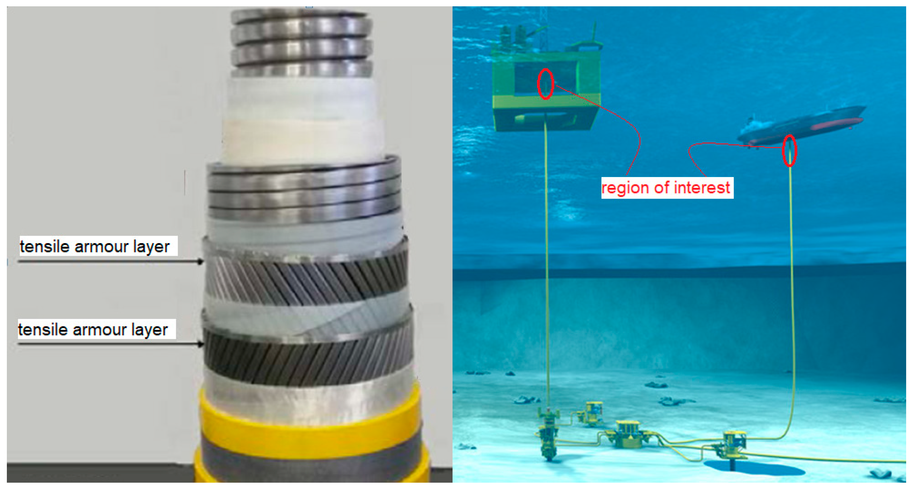
  1. Costa, C.H.O.; Roitman, N.; Magluta, C.; Ellwangwer, G.B. Caracterização das propriedades mecânicas das Camadas de um Riser Felxível. In Proceedings of the 2° Congresso Brasileiro de P&D em Petróleo & Gás, Rio de Janeiro, Brazil, 15–18 June 2003. [Google Scholar]
  2. Li, J.Y.; Qiu, Z.X.; Ju, J.S. Numerical Modeling and Mechanical Analyses of Flexible Risers. Math. Probl. Eng. 2015, 1–7. [Google Scholar]
  3. Balageas, D.; Fritzen, C.P.; Güemes, A. Structural Health Monitoring, 1st ed.; ISTE Ltd.: London, UK, 2006. [Google Scholar]
  4. Raghavan, A. Guided-Wave Structural Health Monitoring. Ph.D. Thesis, University of Michigan, Ann Arbor, MI, USA, 2007. [Google Scholar]
  5. Staszewski, W.J. Structural Health Monitoring Using Guided Ultrasonic Waves. In Advances in Smart Technologies in Structural Engineering; Holnicki-Szulc, J., Soares, C.A.M., Eds.; Springer: New York, NY, USA, 2004; pp. 117–162. [Google Scholar]
  6. Rose, J.L. Ultrasonic Guided Waves in Solid Media; Cambridge University Press: New York, NY, USA, 2014. [Google Scholar]
  7. Eagle, D.M. Fundamentals of Acoustic Emission Testing: Wave Propagation. In NDT Handbook Vol. 6, 3rd ed.; Moore, P.O., Ed.; American Society for Nondestructive Testing Inc.: Columbus, OH, USA, 2005; pp. 79–99. [Google Scholar]
  8. Auld, A.B. Acoustic Fields and Waves in Solids; Wiley: New York, NY, USA, 1973; Volume II. [Google Scholar]
  9. Achenbach, J.D. Wave Propagation in Elastic Solids; Elsevier: Amsterdam, The Nederlands, 1973. [Google Scholar]
  10. Mindlin, R.D.; Fox, E.A. Vibrations and Waves in Elastic Bars of Rectangular Cross Section. J. Appl. Mech. ASME 1960, 27, 152–158. [Google Scholar] [CrossRef]
  11. Graff, K.F. Wave Motion in Elastic Solids; Dover Publications: New York, NY, USA, 1975. [Google Scholar]
  12. Morse, R.W. The Velocity of Compressional Waves in Rods of Rectangular Cross Section. JASA 1950, 22, 219–223. [Google Scholar] [CrossRef]
  13. Cegla, F.B. Energy concentration at the center of large aspect ratio rectangular waveguides at high frequencies. JASA 2008, 123, 4218–4226. [Google Scholar] [CrossRef] [Green Version]
  14. Lamb, H. On Waves in an Elastic Plate. Proc. R. Soc. Lond. 1917, 648, 114–128. [Google Scholar]
  15. Bruneau, M.; Potel, C. Materials and Acoustic Handbook; ISTE: London, UK, 2006. [Google Scholar]
  16. Duan, W.; Gan, T. Investigation of guided wave properties of anisotropic composites laminates using a semi-analytical finite element method. Compos. Part B. 2019, 150, 144–156. [Google Scholar] [CrossRef]
  17. Mindlin, R.D.; Deresiewicz, H. Timoshenko’s Shear Coefficient for Flexural Vibrations of Beams; Technical Report; Columbia University: New York, NY, USA, 1953. [Google Scholar]
  18. Abramson, H.N.; Plass, H.J.; Ripperger, E.A. Stress wave propagation in rods and beams. Arch. Appl. Mech. 1958, 5, 111–194. [Google Scholar] [CrossRef]
  19. Lowe, M.S.J.; Pavlakovic, B.N. Disperse User Manual, Version 2.0.11d Imperial College of Science; Technology and Medicine: London, UK, 2001. [Google Scholar]
  20. Hayashi, T.; Song, W.; Rose, J.L. Guided wave dispersion curves for a bar with an arbitrary cross-section, a rod and rail example. Ultrasonics 2003, 41, 175–183. [Google Scholar] [CrossRef]
  21. Predoi, M. Guided waves dispersion equations for orthotropic multilayered pipes solved using standard finite elements code. Ultrasonics 2014, 54, 1825–1831. [Google Scholar] [CrossRef]
  22. Bartoli, I.; Marzani, A.; Di Scalea, F.L.; Viola, E. Modeling wave propagation in damped waveguides with arbitrary cross-section. J. Sound Vib. 2006, 205, 685–707. [Google Scholar] [CrossRef]
  23. Lagasse, P.E. Higher-order finite-element analysis of topographic guides supporting elastic surface waves. JASA 1973, 53, 1116–1122. [Google Scholar] [CrossRef]
  24. Aalami, B. Waves in prismatic guides of arbitrary cross section. J. Appl. Mech. 1973, 40, 1067–1072. [Google Scholar] [CrossRef]
  25. Sorohan, S.; Constatantin, N.; Gavan, M. Anghel Extraction of dispersion curves for waves propagating in free complex waveguides by finite element codes. Ultrasonics 2011, 51, 503–515. [Google Scholar] [CrossRef] [PubMed]
  26. Packo, P.; Uhl, T.; Staszewski, W.J. Generalizaded semi-analytical finite difference method for dispersion curve calculation and numerical dispersion analysis for Lamb waves. JASA 2014, 136, 993–1002. [Google Scholar] [CrossRef]
  27. Zuo, P.; Zhou, Y.; Fan, Z. Numerical studies of nonlinear ultrasonic guided waves in uniform waveguides with arbitrary cross sections. AIP Adv. 2016, 6, 075–207. [Google Scholar] [CrossRef] [Green Version]
  28. Pedroi, M.; Castaings, M.; Hosten, B.; Bacon, C. Wave propagation along transversely periodic structures. JASA 2007, 121, 1935–1944. [Google Scholar] [CrossRef]
  29. COMSOL Multiphysics Reference Manual Version 4.4; COMSOL A. B. USA: Burlington, MA, USA, 2013.
  30. Castellaro, S. The complementarity of H/V and dispersion curves. Geophysics 2016, 81, 323–338. [Google Scholar] [CrossRef]
  31. Thierry, V.; Mesnil, O.; Chronopoulos, D. Experimental and numerical determination of the wave dispersion characteristics of complex 3D woven composites. Ultrasonics 2020, 103. [Google Scholar] [CrossRef]
  32. Thierry, V.; Brown, L.; Chronopoulos, D. Multi-scale wave propagation modelling for two-dimensional periodic textile composites. Compos. Part B 2018, 150, 144–156. [Google Scholar] [CrossRef] [Green Version]
  33. Groth, E.B. Propagação de ondas de tensão em hastes retangulares no intervalo de frequência de (0;100 [kHz]). Master’s Thesis, Federal University of Rio Grande do Sul, Porto Alegre, Brazil, 2015. [Google Scholar]
  34. Ansys ANSYS Mechanical User’s Guide; Ansys Inc.: Canonsburg, PA, USA, 2013.
  35. Alleyne, D.; Cawley, P. A two-dimensional Fourier transform method for the measurement of propagating multimode signals. JASA 1990, 89, 1159–1168. [Google Scholar] [CrossRef]
  36. Groth, E.; Clarke, T.R.; Iturrioz, I. The Dispersion Curve Applied in Guided Wave Propagation in Prismatic Rods. Lat. Am. J. Solids Struct. 2018, 15, 1–15. [Google Scholar] [CrossRef]
  37. ABNT NBR NM 87:2000. Carbon Steel and Alloy Steel for General Engineering Purpose-Designation and Chemical Composition; Brazilian Association of Technical Norms: Janeiro, Brazil, 2000. [Google Scholar]
  38. National Labview User Manual; National Instruments Corporation: Austin, TX, USA, 2003.
  39. MatLab MATLAB Primer; The MathWors, Inc.: Natick, MA, USA, 2017.
  40. Barker, L.M. Laser Interferometry in Shock-wave Research. Exp. Mech. 1972, 12, 209–215. [Google Scholar] [CrossRef]
  41. Stern, A. Sampling of linear canonical transformed signals. Signal Process 2006, 86, 1421–1425. [Google Scholar] [CrossRef]
  42. Hallquist, J.O. LS-DYNA Theory Manual; Livermore Software Technology Corporation: Livermore, CA, USA, 2006. [Google Scholar]
  43. Barauskas, R.; Abraitiene, A. Computational analysis of impact of bullet against the multilayer fabrics in LS-DYNA. Int. J. Impact Eng. 2007, 34, 1286–1305. [Google Scholar] [CrossRef]
  44. Li, J.; Fang, X. Stress Wave Analysis and optical force measurement of Servo-Hydraulic Machine for High Strain Rate Testing. Exp. Mech. 2014, 54, 1497–1501. [Google Scholar] [CrossRef]
  45. Thurston, R.N. Elastic Waves in Rods and Optical Fibers. J. Sound Vib. 1992, 159, 441–467. [Google Scholar] [CrossRef]
  46. Yu, F.T.S.; Yin, S. Fiber Optic Sensors; Marcel Dekker, Inc.: New York, NY, USA, 2002. [Google Scholar]
  47. Boffa, N.D.; Monaco, E.; Ricci, F. Memmolo Hybrid Strctural Health Monitoring on composite plates with embedded and secondary bonded Fiber Gratings arrays and piezoelectric patches. In Proceedings of the 11th International Symposium on NDT in Aerospace, Paris-Saclay, France, 13–15 November 2019. [Google Scholar]
  48. Mohammad, A.; Matheson, C.; Ridgeway, L. Application of piezoelectric MFC sensors and Fiber Bragg Grating sensors in structural health monitoring of composite materials. In Proceedings of the Sensors and Smart Structures Technologies for Civil, Mechanical, and Aerospace Systems, SPIE, CA, USA, 9 July 2019. [Google Scholar]
  49. Grosse, C.U.; Ohtsu, M. Acoustic Emission Testing; Springer: Berlin/Heidelberg, Germany, 2008. [Google Scholar]
  50. Carpinteri, A.; Lacidogna, G.; Puzzi, S. From criticality to final collapse: Evolution of the b-value from 1.5 to 1.0. Chaos Solitons Fractals 2009, 41, 843–853. [Google Scholar] [CrossRef]
  51. Riera, J.D. Local effects in impact problems on concrete structures. In Proceedings of the Conference on Structural Analysis and Design of Nuclear Power Plants, Porto Alegre, Brazil, October 1984; Volume 3, p. 83. [Google Scholar]
  52. Hillerborg, A. A Model for Fracture Analysis; Cod. LUTVDG/TV BM-3005): Lund, Swede, 1978; pp. 1–8. [Google Scholar]
  53. Kosteski, L.; Iturrioz, I.; Batista, R.G.; Cisilino, A.P. The truss-like discrete element method in fracture and damage mechanics. Eng. Comp. 2011, 6, 765–787. [Google Scholar] [CrossRef]
  54. Kosteski, L.E.; Barrios, R.; Iturrioz, I. Crack propagation in elastic solids using the truss-like discrete element method. Int. J. Fract. 2012, 174, 139–161. [Google Scholar] [CrossRef]
  55. Kosteski, L.E.; Iturrioz, I.; Cisilino, A.P.; D’ambra, R.B.; Pettarin, V.; Fasce, L.; Frontini, P. A lattice discrete element method to model the falling-weight impact test of PMMA specimens. Int. J. Impact Eng. 2016, 87, 120–131. [Google Scholar] [CrossRef]
  56. Kosteski, L.E.; Iturrioz, I.; Lacidogna, G.; Carpinteri, A. Size effect in heterogeneous materials analyzed through a lattice discrete element method approach. Eng. Fract. Mech. 2020, 232. [Google Scholar] [CrossRef]
  57. Birck, G.; Iturrioz, I.; Lacidogna, G.; Carpinteri, A. Damage process in heterogeneous materials analyzed by a lattice model simulation. Eng. Fail. Anal. 2016, 70, 157–176. [Google Scholar] [CrossRef]
  58. Iturrioz, I.; Lacidogna, G.; Carpinteri, A. Experimental analysis and truss-like discrete element model simulation of concrete specimens under uniaxial compression. Eng. Fract. Mech. 2013, 110, 81–98. [Google Scholar] [CrossRef]
  59. Iturrioz, I.; Lacidogna, G.; Carpinteri, A. Acoustic emission detection in concrete specimens: Experimental analysis and lattice model simulations. Int. J. Damage Mech. 2013, 23, 327–358. [Google Scholar] [CrossRef]
  60. Schumacher da Silva, G.; Kosteski, L.E.; Iturrioz, I. Analysis of the failure process by using the Lattice Discrete Element Method in the Abaqus environment. Theor. A Fract. Mech. 2020, 107. [Google Scholar] [CrossRef]
  61. Borges Favaro, M. Correlação Numérica-Experimental da Redução da Vida em Fadiga de Dutos Flexíveis Operando com Anular Alagado na Presença de CO2. DSc. Thesis, Federal University of Rio Grande do Sul, UFRGS, Porto Alegre, Brazil, 2017. Available online: https://www.lume.ufrgs.br/handle/10183/172110 (accessed on 20 June 2020).
  62. Groth, E.; Schumajer, G.; Iturrioz, I.; Kosteski, L.E.; Clarke, T.R. Acoustic Emission Propagation in a Prismatic Guided Wave: Simulations Using Lattice Discrete Element Method. In Progress of the Acoustic Emission IIIAE, Proceedings of the International Conference on Acoustic Emission, Kyoto, Japan, 5–8 December 2016; Volume 1, pp. 1–6. [Google Scholar]
  63. Moore, P.O. Acoustical Emission testing Handbook, 3rd ed.; 6 American Society of non destructive testing; Library of Congress: Washington, DC, USA, 2005; ISBN 1-57117-106-1. [Google Scholar]
  64. Lacidogna, G.; Piana, G.; Accornero, F.; Carpinteri, A. Multi-technique damage monitoring of concrete beams: Acoustic Emission, Digital Image Correlation, Dynamic Identification. Constr. Build. Mater. 2020, 242, 118114. [Google Scholar] [CrossRef]
  65. Carpinteri, A.; Lacidogna, G.; Corrado, M.; Di Battista, E. Cracking and crackling in concrete-like materials: A dynamic energy balance. Eng. Fract. Mech. 2016, 155, 130–144. [Google Scholar] [CrossRef]
Figure 1. (a) The different layers of a typical riser, (b) the region of the riser that could be monitored using techniques based on guided wave propagation.
Applsci 10 04401 g001
Figure 2. Modes S n and A n   of a rectangular waveguide, with section 15 × 5 [mm], in the frequency range [0, 1] MHz. Notice that in this graph the wave number is defined as k = 2π/λ [m−1].
Applsci 10 04401 g002
Figure 3. The dispersion curves computed by [11], for a waveguide of rectangular section 15 × 5 [mm]. Notice that in this graph the wave number is defined as k = 2π/λ [m−1].
Applsci 10 04401 g003
Figure 4. Dispersion curves of the rectangular stem computed from the two plates overlapping as presented [13], one considering a thickness of 15 [mm] and the other one a thickness of 5 [mm]. The axis orientation is presented in Figure 5g. Notice that in this graph the wave number is defined as k = 2π/λ [m−1].
Applsci 10 04401 g004
Figure 5. (a) Dispersion curves computed using the Pedroi et al. method presented in [28]. Displacement field of (b) second torsional, (c) longitudinal, (d) torsional, (e) flexural (around Axis (2)), (f) flexural wave mode (around Axis (3)). (g) The waveguide scheme with the reference axes indicated. Notice that in this graph the wave number is defined as k = 2π/λ [m−1].
Applsci 10 04401 g005
Figure 6. Scheme showing the portion of the waveguide modeled using 3D finite element analysis (FEM) for the Sorohan et al. [25] in the semi-analytical finite element method (SAFE) implementation.
Applsci 10 04401 g006
Figure 7. Results using the Sorohan et al. [25] SAFE method, the dispersion curves and the displacement field of each mode. Notice that in this graph the wave number is defined as k = 2π/λ [m−1].
Applsci 10 04401 g007
Figure 8. Frequency response of the piezoelectric transducers used during the tests.
Applsci 10 04401 g008
Figure 9. Details of the experimental setup: (a) laser vibrometer position to obtain displacements u1 and u2. Using piezoelectric ceramics (PZT) with longitudinal polarization to induce longitudinal and flexural around Axis 3 wave modes. (b) Laser vibrometer position to obtain displacements u2 and u3. Using PZT with transversal polarization to induce the flexural around Axis 2 and torsional wave modes. The black line indicates the scanning region, and the green arrow shows the polarization of the PZT transducer. (c) Detail of the PZT transducer glued to the beam tip. (d) The platform where the vibrometers are fixed (the red arrows indicate the degrees of freedom of the platform). (e) Diagram of the experimental setup where the main dimensions were indicated.
Applsci 10 04401 g009
Figure 10. A tone burst with the main frequency of 80 KHz in longitudinal direction. Experimental results: (a) displacements measured in a point over the scan line where T is the period of each wave propagation mode. (b) Displacements over the scan line at a specific time. Numerical results: (c) amplitude displacement in the frequency vs. wave number dominium (with a black line indicating the dispersion curves). (d) Bar analyzed with the map of displacement on it, at a specific time. (e) Transversal section with the spatial distribution of two wave modes. (f) Tridimensional mode views.
Applsci 10 04401 g010
Figure 11. A tone burst with the main frequency of 80 KHz in transversal direction. Experimental results: (a) Displacements measured in a point over the scan line where T is the period of each wave propagation mode. (b) displacement over the scan line at a specific time. Numerical results: (c) amplitude displacement in the frequency vs. wave number dominium (with a black line indicating the dispersion curves). (d) Bar analyzed with the map of displacement on it, in a specific time. (e) Transversal section with the spatial distribution of two wave modes. (f) Tridimensional mode views.
Applsci 10 04401 g011
Figure 12. Comparison made between experimental results (dots) and theoretical dispersion curves obtained using SAFE [28] implemented in the COMSOL [29] environment (lines). Moreover, l = longitudinal mode, f2 = flexion around 2, t = torsion, f3 = flexion around Axis 3. Notice that, in this plot the wave number is defined as k = (1/λ)
Applsci 10 04401 g012
Figure 13. Comparison made between the analytical beam model [11] (color lines) and SAFE [28] solution (grey lines). (l: longitudinal, t: torsional, f2: flexion around Axis 2, f3: flexion around Axis 3. Notice that in this graph the wave number is defined as k = 2π/λ [m−1].
Applsci 10 04401 g013
Figure 14. Comparison between SAFE method [28] (grey lines) and the superposition of the plate solutions [13] (color lines). Notice that in this graph the wave number is defined as k = 2π/λ [m−1].
Applsci 10 04401 g014
Figure 15. Scattering curves of three different sections height × width. (The blue dots in the graph indicate no fundamental modes). Notice that in this graph the wave number is defined as k = 2π/λ [m−1].
Applsci 10 04401 g015
Figure 16. Experimental setup used in the assessment made using optical fiber sensors to capture the propagation of mechanical waves in a rectangular rod.
Applsci 10 04401 g016
Figure 17. Collected Signal with the fiber Bragg grating with a tone burst excitation (57 KHz and 7 cycles).
Applsci 10 04401 g017
Figure 18. The lattice discrete element method (LDEM); (a) basic cubic module, (b) generation of a prismatic body, and (c) bilinear constitutive model where the damage is taken into account.
Applsci 10 04401 g018
Figure 19. The pre-fissured prismatic metallic waveguide modeled with LDEM + FEM. The boundary conditions are also depicted.
Applsci 10 04401 g019
Figure 20. Results in the Frequency vs. wave-number domain. (a) in Mode I, (b) in Mode II, (c) in Mode III. (d) The spatial distribution of the three modes of fissure crack propagation, AE emitted from the pre-fissure solicited.
Applsci 10 04401 g020
Figure 21. Information about the acoustic generic emission events simulated: when a typical event happened: (a) dissipated energy increments Ed and its Ed evolution during the process simulated. (b) Kinetic energy Ek and the evolution of its increment Ek during the process simulated. (c) The typical acoustic emission event, A shows by means of the acceleration captured by a sensor (gray line), the Ek and Ed evolution during the process simulated. (d) Detail of a typical fissure propagation simulated with the numerical model used (figure edited from [59]).
Applsci 10 04401 g021
Table 1. Expressions of the dispersion curves considering the rod as a beam.
ModeAnalytic Dispersion Function
Longitudinal ω = k E ρ
Torsional ω = k C t J ρ
Flexural ω = k 2 E I ρ A

