Robust-Extended Kalman Filter and Long Short-Term Memory Combination to Enhance the Quality of Single Point Positioning

 ,
, 
Abstract
:1. Introduction
2. Single Point Positioning Technology
3. Robust Extended Kalman Filter
3.1. Robust Extended Kalman Filter Model
3.2. MM Estimation Theory
3.3. Iterative Reweighted Least Squares Algorithm
- Find an initial estimate
- Estimate the vector for initial residuals of the observations :
- Define the initial scale value [33]where “” stands for the median function computed on the residuals vector .
- Estimate the initial diagonal weight matrix by MM-Estimation.where ; n being the number of observations.
- While (j is iteration)
- (a)
- Update the value of the matrix at the iteration with
- (b)
- Solve the estimated state using the weighted least-squared method
- (c)
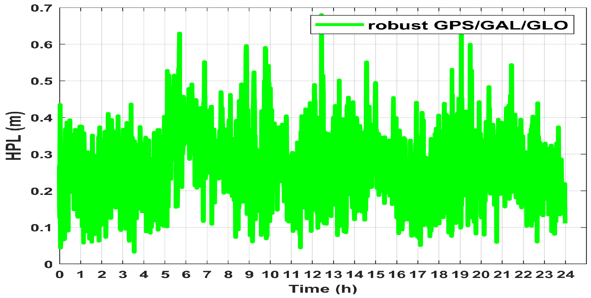
- Calculate the HPL (in Section 3.4)
- (d)
- If ; break
- (e)
- If ; continue
- (f)
- Update the estimated residuals
- (g)
- Calculate the scale value
- (h)
- Recalculate the diagonal weighted matrix using MM-Estimation:
- (i)
- Go to step (a)
- End
- If then the estimated positions are accepted, (HAL: Horizontal Alert Limit)If not, they are rejected.
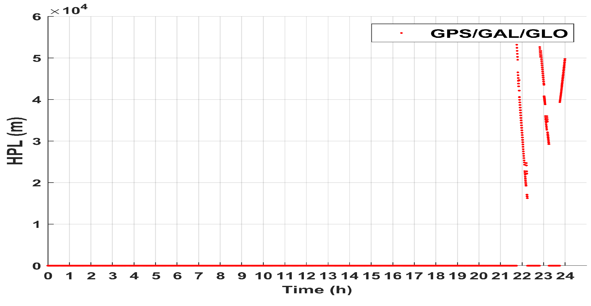
3.4. RAIM Algorithm
4. Experimental Results of Applying Robust-EKF
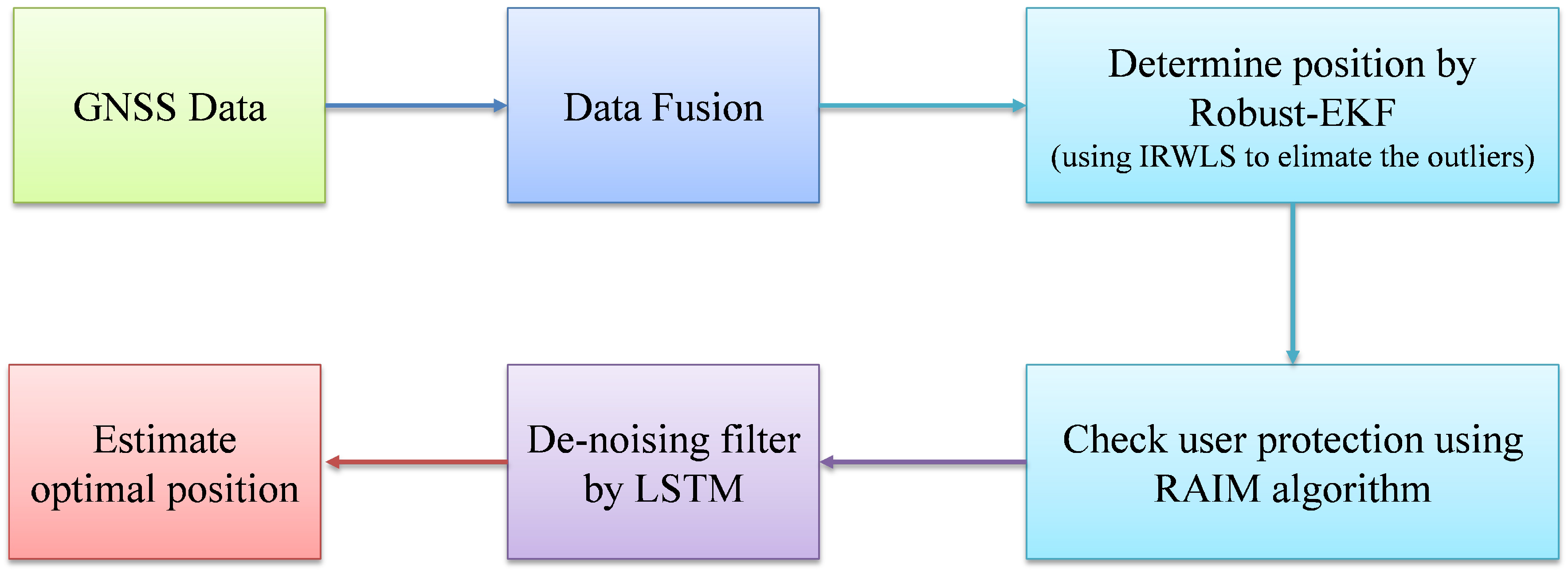
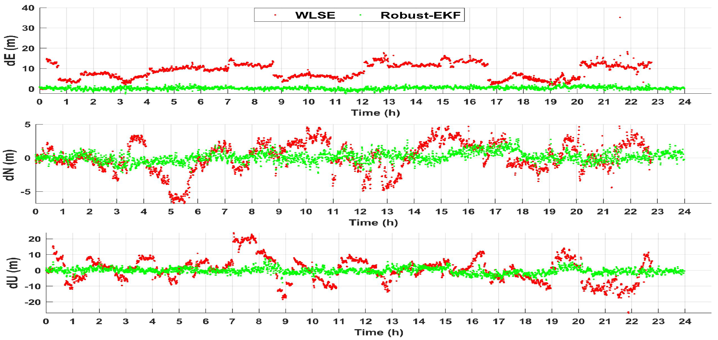
4.1. Applying Robust-EKF
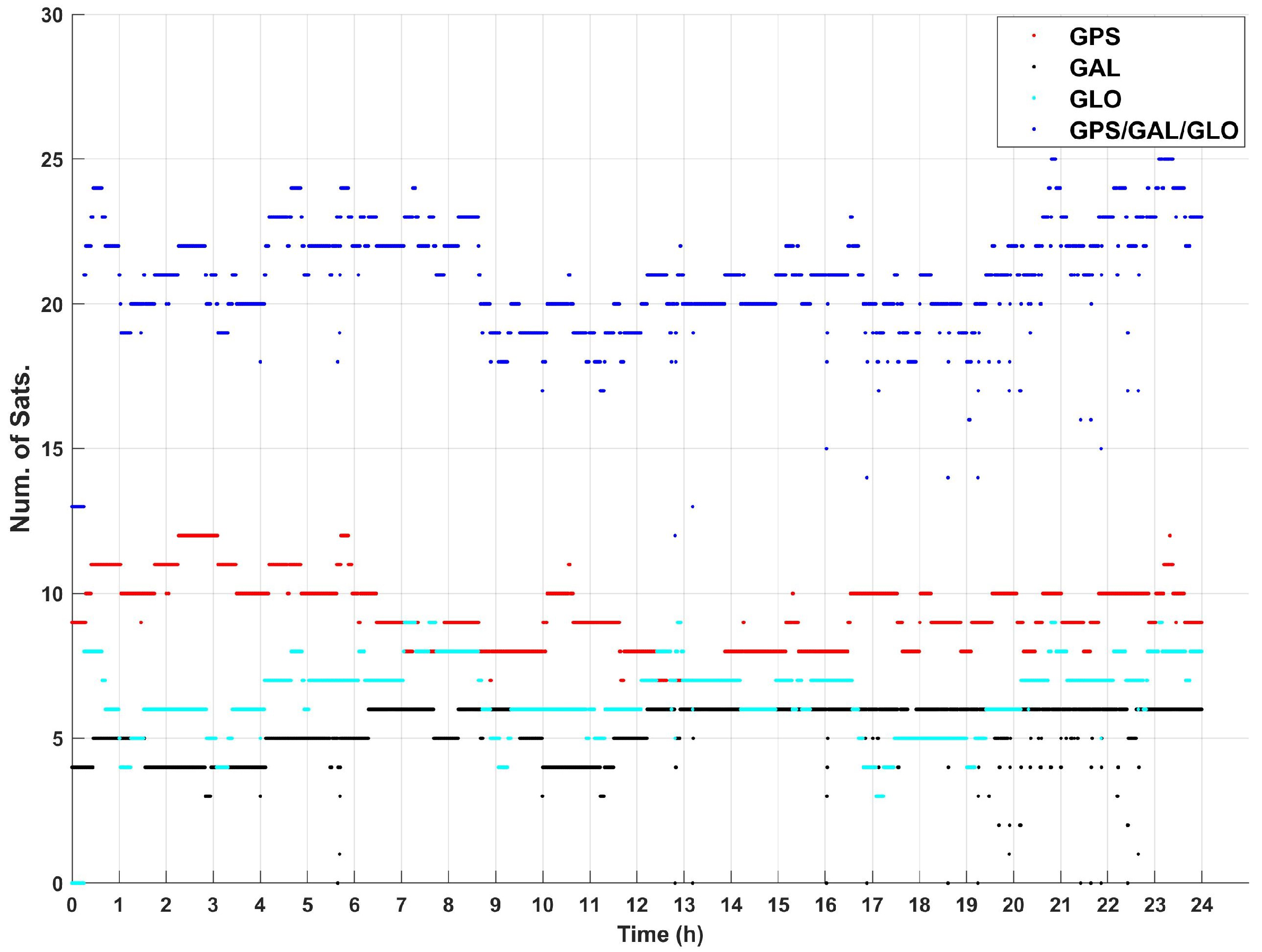
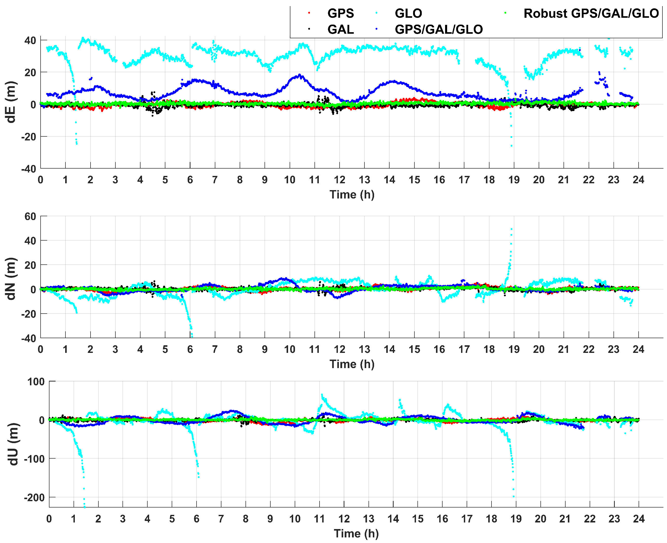
4.2. Experimental Results
- Scenario #1: Navigation solution based on GPS data,
- Scenario #2: Navigation solution based on Galileo data,
- Scenario #3: Navigation solution based on GLONASS data,
- Scenario #4: Navigation solution based on GPS/Galileo/GLONASS data,
- Scenario #5: Navigation solution based on robust-EKF GPS/Galileo/GLONASS data.
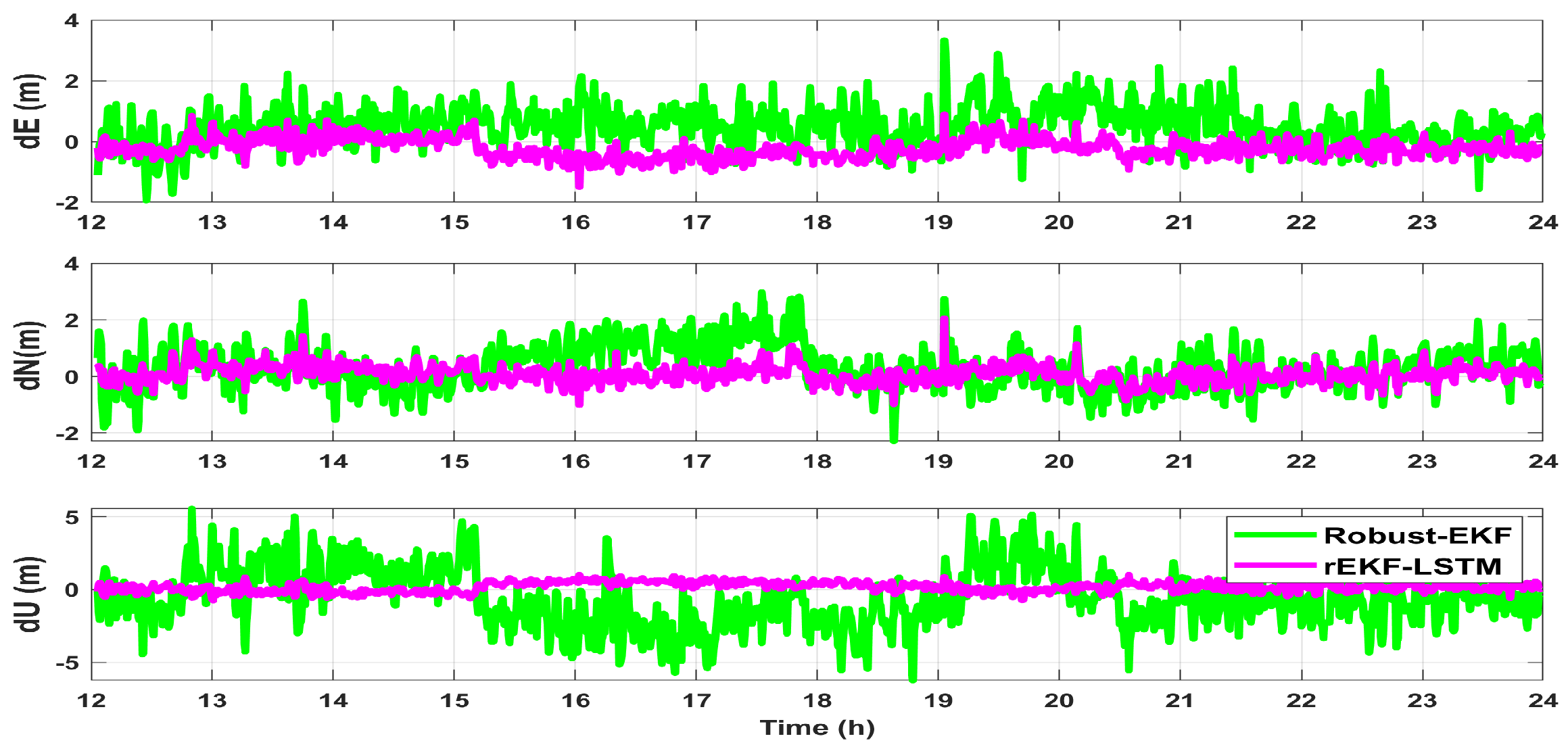
5. De-Noising Filter Method and Experimental Results
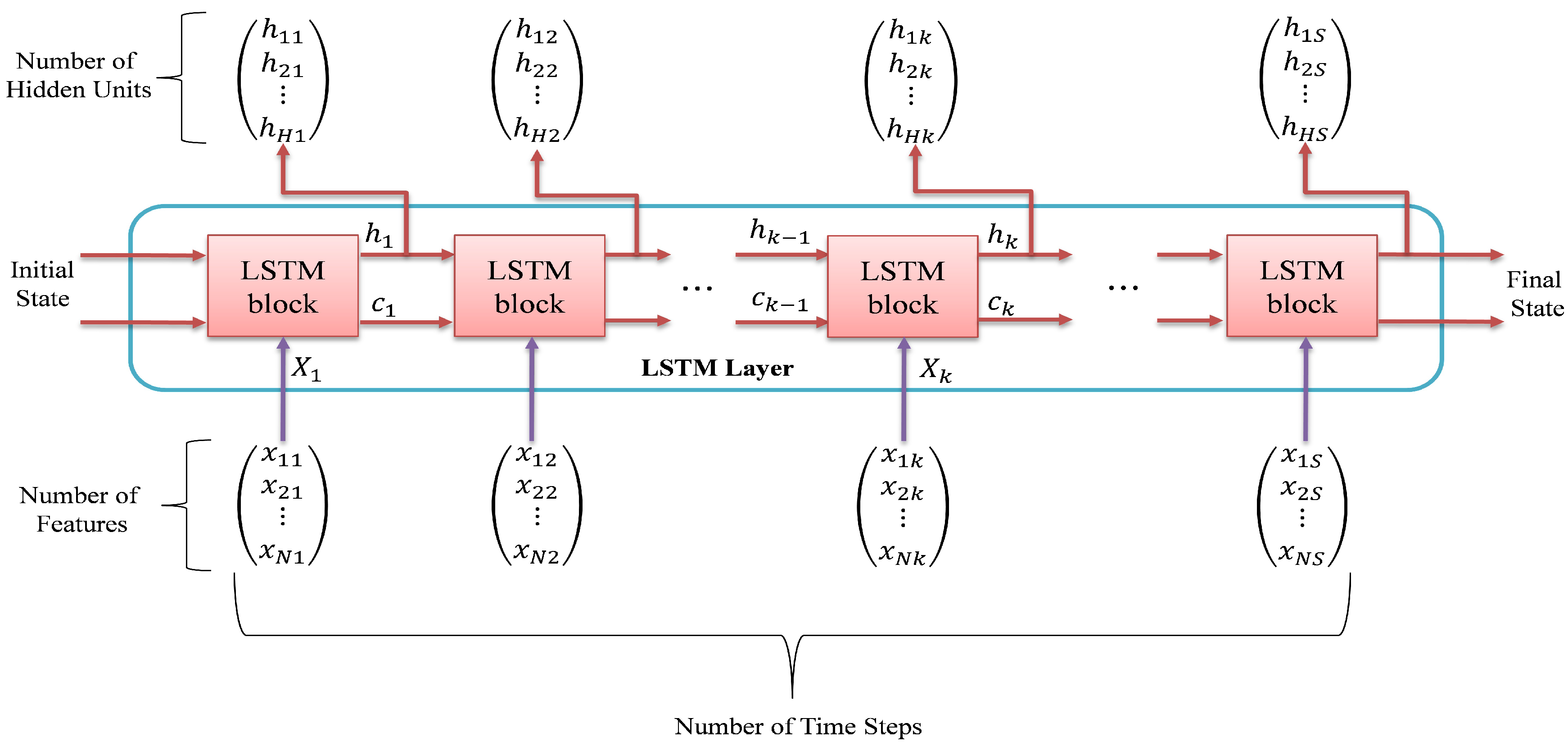
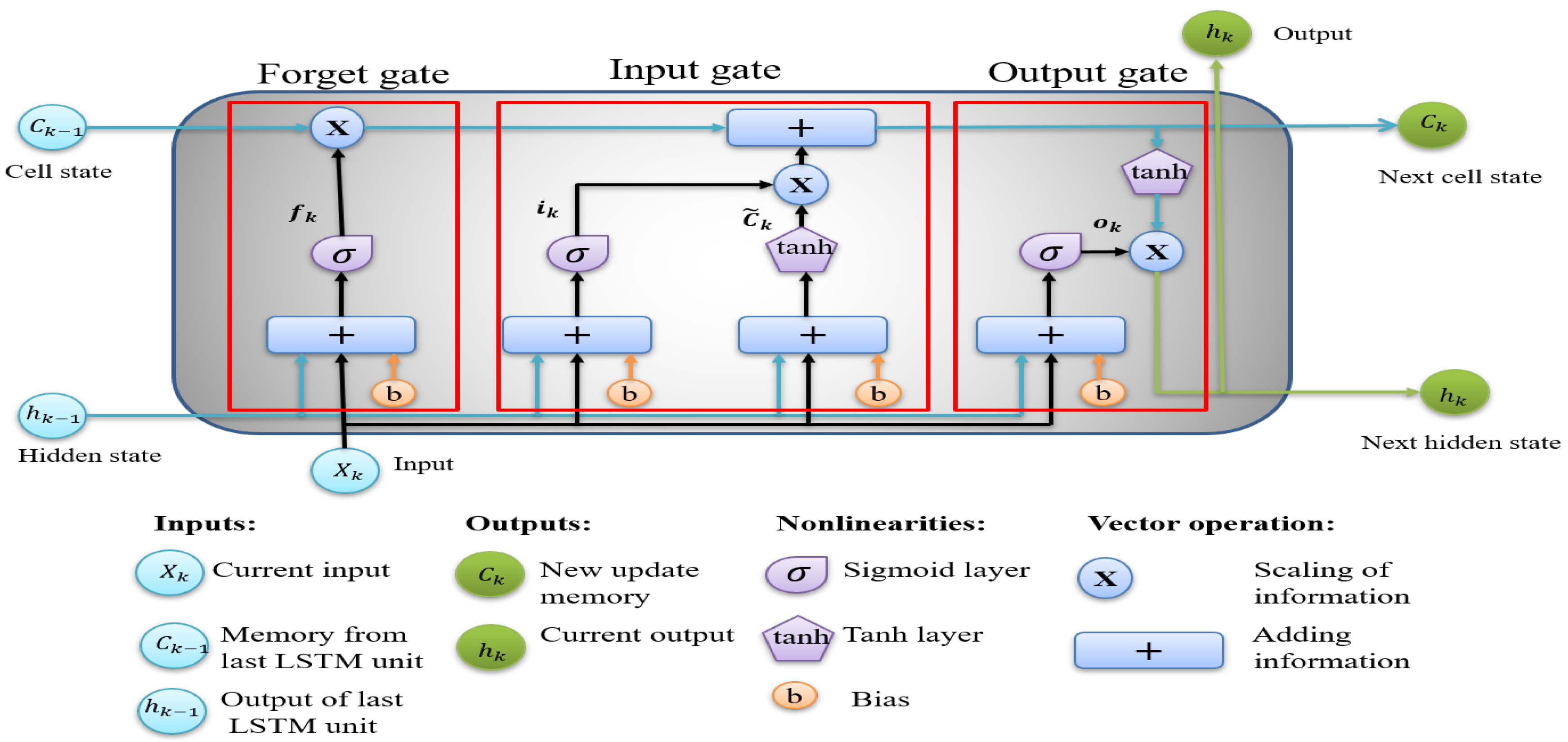
5.1. De-Noising Filter Model
5.2. Experimental Results
6. Conclusions and Perspectives
Author Contributions
Funding
Acknowledgments
Conflicts of Interest
References
- Zhang, X.; Huang, Z.; Li, R. RAIM analysis in the position domain. In Proceedings of the IEEE/ION Position, Location and Navigation Symposium, Indian Wells, CA, USA, 4–6 May 2010; pp. 53–59. [Google Scholar] [CrossRef]
- Hewitson, S.; Lee, H.K.; Wang, J. Localizability analysis for GPS/Galileo receiver autonomous integrity monitoring. J. Navig. 2004, 57, 245–259. [Google Scholar] [CrossRef] [Green Version]
- Blanch, J.; Ene, A.; Walter, T.; Enge, P. An optimized multiple hypothesis RAIM algorithm for vertical guidance. In Proceedings of the 20th International Technical Meeting of the Satellite Division of the Institute of Navigation, Fort Worth, TX, USA, 25–28 September 2007; Volume 3, pp. 2924–2933. [Google Scholar]
- Tay, S.; Marais, J. Weighting models for GPS Pseudorange observations for land transportation in urban canyons. In Proceedings of the 6th European Workshop on GNSS Signals and Signal Processing, Munich, Germany, 5–6 December 2013. [Google Scholar]
- Rahemi, N.; Mosavi, M.R.; Abedi, A.A.; Mirzakuchaki, S. Accurate Solution of Navigation Equations in GPS Receivers for Very High Velocities Using Pseudorange Measurements. Adv. Aerosp. Eng. 2014, 2014, 435891. [Google Scholar] [CrossRef]
- Tabatabaei, A.; Mosavi, M.R.; Khavari, A.; Shahhoseini, H.S. Reliable Urban Canyon Navigation Solution in GPS and GLONASS Integrated Receiver Using Improved Fuzzy Weighted Least-Square Method. Wirel. Pers. Commun. 2017, 94, 3181–3196. [Google Scholar] [CrossRef]
- Li, J.; Wu, M. The improvement of positioning accuracy with weighted least square based on SNR. In Proceedings of the 5th International Conference on Wireless Communications, Networking and Mobile Computing (WiCOM), Beijing, China, 24–26 September 2009; pp. 9–12. [Google Scholar] [CrossRef]
- Tan, T.N.; Khenchaf, A.; Comblet, F. Estimating Ambiguity and Using Model Weight To Improve the Positioning Accuracy of a Stand-alone Receiver. In Proceedings of the 13th European Conference on Antennas Propagation (EuCAP 2019), Krakow, Poland, 31 March–5 April 2019; Volume 1. [Google Scholar]
- Tan, T.N.; Khenchaf, A.; Comblet, F.; Franck, P.; Champeyroux, J.M.; Reichert, O. GPS/GLONASS Data Fusion and Outlier Elimination to Improve the Position Accuracy of Receiver. In Proceedings of the 2019 IEEE Conference on Antenna Measurements & Applications (CAMA), Bali, Indonesia, 23–25 October 2019; Volume 805, pp. 191–194. [Google Scholar] [CrossRef]
- Wang, Y.; Jie, H.; Cheng, L. A Fusion Localization Method based on a Robust Extended Kalman Filter and Track-Quality for Wireless Sensor Networks. Sensors 2019, 19, 3638. [Google Scholar] [CrossRef] [PubMed] [Green Version]
- Fang, H.; Haile, M.A.; Wang, Y. Robust Extended Kalman Filtering for Systems with Measurement Outliers. arXiv, 2019; arXiv:1904.00335. [Google Scholar]
- Perälä, T.; Piché, R. Robust extended Kalman filtering in hybrid positioning applications. In Proceedings of the 4th Workshop on Positioning, Navigation and Communication, WPNC’07—Workshop Proceedings, Hannover, Germany, 22 March 2007; pp. 55–63. [Google Scholar] [CrossRef]
- Gao, Z.; Li, Y.; Zhuang, Y.; Yang, H.; Pan, Y.; Zhang, H. Robust kalman filter aided GEO/IGSO/GPS raw-PPP/INS tight integration. Sensors 2019, 19, 417. [Google Scholar] [CrossRef] [PubMed] [Green Version]
- Wang, J.; Xu, C.; Wang, J. Applications of Robust Kalman Filtering Schemes in GNSS Navigation. In Proceedings of the International Symposium on GPS/GNSS, Tokyo, Japan, 11–14 Novembre 2008. [Google Scholar]
- Gaglione, S.; Angrisano, A.; Crocetto, N. Robust Kalman Filter applied to GNSS positioning in harsh environment. In Proceedings of the European Navigation Conference (ENC 2019), Warsaw, Poland, 9–12 April 2019; pp. 1–6. [Google Scholar] [CrossRef]
- Kumar, P. Robust Kalman Filter Using Robust Cost Function. Master’s Thesis, Deparment of Electronics and Communication Engineering, National Institute of Technology, Rourkela, Indian, 2015. [Google Scholar]
- Gandhi, M.A.; Mili, L. Robust Kalman Filter based on a generalized maximum-likelihood-type estimator. IEEE Trans. Signal Process. 2010, 58, 2509–2520. [Google Scholar] [CrossRef]
- Zhao, J.; Netto, M.; Mili, L. A Robust Iterated Extended Kalman Filter for Power System Dynamic State Estimation. IEEE Trans. Power Syst. 2017, 32, 3205–3216. [Google Scholar] [CrossRef]
- Yuliana, S.; Hasih, P.; Sri Sulistijowati, H.; Twenty, L. M Estimation, S Estimation, and MM Estimation in Robust Regression. Int. J. Pure Appl. Math. 2014, 91, 349–360. [Google Scholar]
- Yohai, Y.J. High Breakdown-point and High Efficiency Robust Estimates for Regression. Ann. Stat. 1986, 14, 590–606. [Google Scholar] [CrossRef]
- Huber, P.J. Robust Statistics; John Wiley and Sons, Inc.: Hoboken, NJ, USA, 2009. [Google Scholar]
- Akram, M.A.; Liu, P.; Wang, Y.; Qian, J. GNSS positioning accuracy enhancement based on robust statistical MM estimation theory for ground vehicles in challenging environments. Appl. Sci. 2018, 8, 876. [Google Scholar] [CrossRef] [Green Version]
- Strang, G.; Borre, S. Algorithms for Global Positioning; Wellesley-Cambridge Press: Wellesley, MA, USA, 2012. [Google Scholar]
- Fang, W.; Jiang, J.; Lu, S.; Gong, Y.; Tao, Y.; Tang, Y.; Yan, P.; Luo, H.; Liu, J. A LSTM algorithm estimating pseudo measurements for aiding INS during GNSS signal outages. Remote Sens. 2020, 12, 256. [Google Scholar] [CrossRef] [Green Version]
- Jiang, C.; Chen, S.; Chen, Y.; Zhang, B.; Feng, Z.; Zhou, H.; Bo, Y. A MEMS IMU de-noising method using long short term memory recurrent neural networks (LSTM-RNN). Sensors 2018, 18, 3470. [Google Scholar] [CrossRef] [PubMed] [Green Version]
- Li, X.; Wu, X. Constructing long short-term memory based deep recurrent neural networks for large vocabulary speech recognition. In Proceedings of the ICASSP, IEEE International Conference on Acoustics, Speech and Signal Processing, Brisbane, Australia, 19–24 April 2015; pp. 4520–4524. [Google Scholar] [CrossRef] [Green Version]
- Kim, H.U.; Bae, T.S. Deep learning-based GNSS network-based real-time kinematic improvement for autonomous ground vehicle navigation. J. Sens. 2019, 2019, 3737265. [Google Scholar] [CrossRef]
- Kim, H.U.; Bae, T.S. Preliminary study of deep learning-based precipitation prediction. J. Korean Soc. Surv. Geod. Photogramm. Cartogr. 2017, 35, 423–429. [Google Scholar] [CrossRef]
- Nicolini, L.; Caporali, A. Investigation on reference frames and time systems in Multi-GNSS. Remote Sens. 2018, 10, 80. [Google Scholar] [CrossRef] [Green Version]
- Gurtner, W.; Estey, L. RINEX The Receiver Independent Exchange Format Version 3.03. In Proceedings of the IGS Workshop 2012, Olsztyn, Poland, 23–27 July 2012; Volume 104, pp. 1–74. [Google Scholar]
- Noureldin, A.; Karamat, T.B.; Georgy, J. Fundamentals of Inertial Navigation, Satellite-Based Positoning and Their Integration; Springer: Berlin/Heidelberg, Germany, 2013. [Google Scholar]
- Hofmann-Wellenhof, B.; Lichtenegger, H.; Wasle, E. GNSS—Global Navigation Satellite Systems: GPS, GLONASS, Galileo and More; Springer: Wien, Austria, 2008. [Google Scholar]
- Ellis, D.M.; Draper, N.P.; Smith, H. Applied Regression Analysis. Appl. Stat. 1968, 17, 83. [Google Scholar] [CrossRef]
- Chiang, K.W.; Chang, H.W.; Li, C.Y.; Huang, Y.W. An Artificial Neural Network Embedded Position and Orientation Determination Algorithm for Low Cost MEMS INS/GPS Integrated Sensors. Sensors 2009, 9, 2586–2610. [Google Scholar] [CrossRef] [Green Version]


| Name | Weight Function |
|---|---|
| Huber | |
| Bi-Tukey | |
| Bi-Square |
| RMS Error (m) | GPS | GAL | GLO | GPS/GAL/GLO | Robust-EKF GPS/GAL/GLO |
|---|---|---|---|---|---|
| RMS-E | 1.42 | 1.34 | 31.00 | 8.11 | 0.74 |
| RMS-N | 1.46 | 1.2 | 6.65 | 2.74 | 0.75 |
| RMS-U | 3.94 | 3.08 | 25.7 | 9.50 | 1.82 |
| 3D-RMS | 4.43 | 3.56 | 40.81 | 12.73 | 2.1 |
| RMS Error (m) | Robust-EKF | rEKF-LSTM |
|---|---|---|
| RMS-E | 0.82 | 0.39 |
| RMS-N | 0.83 | 0.32 |
| RMS-U | 2.04 | 0.36 |
| 3D-RMS | 2.35 | 0.62 |
| RMS Error (m) | GPS | GAL | GLO | GPS/GAL/GLO | Robust-EKF GPS/GAL/GLO | rEKF-LSTM |
|---|---|---|---|---|---|---|
| RMS-E | 1.43 | 1.21 | 30.71 | 7.08 | 0.82 | 0.39 |
| RMS-N | 1.58 | 1.19 | 6.18 | 2.27 | 0.83 | 0.32 |
| RMS-U | 3.32 | 3.07 | 21.10 | 8.18 | 2.04 | 0.36 |
| 3D-RMS | 3.95 | 3.50 | 37.76 | 11.05 | 2.35 | 0.62 |
| Base Station | RMS Error (m) | GPS | GAL | GLO | GPS/GAL/GLO | Robust-EKF GPS/GAL/GLO | rEKF-LSTM |
|---|---|---|---|---|---|---|---|
| RMS-E | 1.12 | 1.36 | 17.76 | 3.40 | 0.72 | 0.73 | |
| AJAC | RMS-N | 1.65 | 1.25 | 9.30 | 4.57 | 0.88 | 0.46 |
| RMS-U | 2.52 | 2.42 | 3.40 | 4.75 | 1.33 | 0.45 | |
| 3D-RMS | 3.21 | 3.04 | 20.33 | 7.42 | 1.75 | 0.97 | |
| RMS-E | 1.14 | 1.38 | 17.39 | 3.42 | 0.67 | 0.75 | |
| GRAC | RMS-N | 1.58 | 1.28 | 11.87 | 5.85 | 0.91 | 0.54 |
| RMS-U | 2.89 | 3.02 | 12.74 | 4.76 | 2.29 | 1.66 | |
| 3D-RMS | 3.49 | 3.56 | 24.6 | 8.28 | 2.55 | 1.89 | |
| RMS-E | 1.59 | 1.07 | 33.12 | 6.62 | 0.68 | 0.51 | |
| LMMF | RMS-N | 1.36 | 0.96 | 11.81 | 1.82 | 0.63 | 0.30 |
| RMS-U | 3.38 | 2.20 | 4.32 | 8.17 | 1.80 | 0.47 | |
| 3D-RMS | 3.96 | 2.63 | 35.43 | 10.67 | 2.02 | 0.76 |
© 2020 by the authors. Licensee MDPI, Basel, Switzerland. This article is an open access article distributed under the terms and conditions of the Creative Commons Attribution (CC BY) license (http://creativecommons.org/licenses/by/4.0/).
Share and Cite
Tan, T.-N.; Khenchaf, A.; Comblet, F.; Franck, P.; Champeyroux, J.-M.; Reichert, O. Robust-Extended Kalman Filter and Long Short-Term Memory Combination to Enhance the Quality of Single Point Positioning. Appl. Sci. 2020, 10, 4335. https://doi.org/10.3390/app10124335
Tan T-N, Khenchaf A, Comblet F, Franck P, Champeyroux J-M, Reichert O. Robust-Extended Kalman Filter and Long Short-Term Memory Combination to Enhance the Quality of Single Point Positioning. Applied Sciences. 2020; 10(12):4335. https://doi.org/10.3390/app10124335
Chicago/Turabian StyleTan, Truong-Ngoc, Ali Khenchaf, Fabrice Comblet, Pierre Franck, Jean-Marc Champeyroux, and Olivier Reichert. 2020. "Robust-Extended Kalman Filter and Long Short-Term Memory Combination to Enhance the Quality of Single Point Positioning" Applied Sciences 10, no. 12: 4335. https://doi.org/10.3390/app10124335