Climatology of the Linke and Unsworth–Monteith Turbidity Parameters for Greece: Introduction to the Notion of a Typical Atmospheric Turbidity Year

Abstract

Solar rays are attenuated by the Earth’s atmosphere. This attenuation can be expressed by the turbidity parameters; two of them are the Linke turbidity factor (T_L) and the Unsworth–Monteith turbidity coefficient (T_UM). In this sudy, both parameters are estimated for 33 sites across Greece, and the notion of a Typical Atmospheric Turbidity Year (TATY) is also introduced. Use of the modified clearness index (k’_t) is made, while a suggestion for a modified diffuse fraction (k’_d) is given. The adoption of the four climatic zones in Greece for energy purposes is made, where the variation of T_L and T_UM is studied during a TATY under all and clear-sky conditions. The analysis shows maximum levels in both parameters in late winter–early spring in morning and evening hours, with minimum values at midday. The intra-annual variation of the parameters shows maximum values around March and August and minimum values in summertime and late winter. Maps of annual mean T_L and T_UM values over Greece show persistent minimum values over Peloponnese and maximum values over South Ionian Sea. Linear expressions of T_UM vs. T_L are derived for all sites under all and clear-sky conditions. Finally, linear expressions for k’_d vs. k’_t are given for all sites and sky conditions.

1. Introduction

Solar radiation reaching the surface of the Earth undergoes attenuation due to the absorption and scattering of the solar rays by the atmospheric constituents [1]. Therefore, the solar radiation levels measured on the surface of the Earth depend on the concentration of water vapor, nitrogen dioxide, ozone, mixed gases and atmospheric aerosols. Although empirical–analytical expressions have been provided in the international literature for the atmospheric transmittances of the first four constituents, such expressions would not have been possible for aerosols if the notion of atmospheric turbidity were not introduced. The atmospheric turbidity expresses the attenuation of solar rays by aerosols. Several indices (called atmospheric turbidity parameters) have been introduced for this purpose; these are the Ångström turbidity coefficient (β) and exponent (α) [2,3,4], the Schüepp turbidity factor (B) [5], the Linke turbidity factor (T_L) [6,7] and the Unsworth–Monteith turbidity coefficient (T_UM) [8].

There is a growing interest in atmospheric turbidity worldwide as this issue is related to air-pollution studies in cities, solar radiation modelling, atmospheric chemistry, and climate studies. Apart from the pioneering works defining the various atmospheric turbidity parameters mentioned above, numerous studies have been carried out since the 1970s. A sample of such studies is given here.

Polavarapu [9] attempted to evaluate T_L for an urban, a suburban, a rural and an arctic station in Canada. Abdelrahman et al. [10] reported T_L levels for a desert environment (Dhahran, Saudi Arabia). Grenier et al. [11] developed a model for deriving T_L by means of updated spectral extraterrestrial irradiances and extinction coefficients of gaseous absorbers. Eaton [12] discussed the influence of atmospheric boundary-layer stability on atmospheric turbidity and optical turbulence in a desert environment. Cucumo et al. [13] studied the variation of the Linke turbidity factor at two Italian localities, while Diabate et al. [14] evaluated the same factor for several sites in Africa. Zakey et al. [15] studied the atmospheric turbidity levels at two sites in Egypt. Hove and Manyumbu [16] estimated the Linke turbidity factor over Zimbabwe. Bilbao et al. [17] studied the turbidity coefficients in central Spain, while Saad et al. [18] reported the spatial and temporal variability of atmospheric turbidity over Tunisia. Ulscka-Kawalkowsa et al. [19] studied the Linke turbidity factor over Warsaw and Belsk, Poland. A recent study [20] has investigated the accuracy of three different methodologies (in essence, different data inventories) in assessing high atmospheric-turbidity episodes over north-central Spain. The authors found that all three methodologies have a 60% coincidence in identifying such episodes.

In Greece, studies about atmospheric turbidity have been conducted mostly for Athens [21,22,23,24,25,26,27] and Thessaloniki [28]. Most of them refer to the Linke turbidity factor. Therefore, there is a gap in recent turbidity studies for Athens and a complete absence of research for Greece as a whole. This gap is intended to be covered in the present work.

The structure of the paper is as follows. Section 2 presents the methodology for calculating the Linke and Unsworth–Monteith turbidity parameters (Section 2.1), as well as the data collection (Section 2.2) and the data processing (Section 2.3). Section 3.1 and Section 3.2 present the month–hour graphs of T_L and T_UM for selected sites under all and clear-sky conditions, respectively. Section 3.3 accounts for the effect of the clearness index on T_L and T_UM, while Section 3.4 refers to the intra-annual variation of T_L and T_UM over Greece under all and clear-sky conditions. Section 4 presents the main conclusions of the study.

2. Materials and Methods

2.1. Methodology

2.1.1. Calculation of the Linke Turbidity Factor, T_L

T_L was introduced by Linke [6,7] as a parameter to indicate how many (hypothetical) clean and dry atmospheres are necessary to derive the observed attenuation of the extraterrestrial radiation caused by the real atmosphere under clear-sky conditions. T_L is typically bounded between 1 and 10. According to Linke:

$$B_e=S\cdot G_{e,o}\cdot sin\gamma \cdot exp(-m^{\prime }\hspace{0.17em}\cdot \overline{k_r}\cdot T_L)$$

(1)

where B_e is the direct horizontal solar radiation equal to G_e - D_e, S is the correction factor for the Sun–Earth distance [29] given by Equation (3), G_e,o is the solar constant equal to 1361.10 Wm⁻² [30], γ is the solar elevation, m’ is the pressure-corrected optical air mass (Equation (5)), which includes the altitude of the site at which T_L is to be estimated, and $\overline{k_r}$ is the mean attenuation of the direct solar radiation due to Rayleigh scattering alone [31,32]. Solving Equation (1) for T_L, we obtain

$$T_L=\frac{ln{G}_{e,o}-ln{B}_e+lnS+lnsin\gamma }{\overline{k_r}\hspace{0.17em}{m}^{\prime }}$$

(2)

in which

$$S=1+0.033\hspace{0.17em}cos\left(\frac{2\hspace{0.17em}\pi \hspace{0.17em}D}{365}\right)$$

(3)

$$\overline{k_r}=6.5567+1.7513\hspace{0.17em}{m}^{\prime }-0.1202\hspace{0.17em}{m}^{\prime }{\hspace{0.17em}}^2+0.0065\hspace{0.17em}{m}^{\prime }{\hspace{0.17em}}^3-0.00013\hspace{0.17em}{m}^{\prime }{\hspace{0.17em}}^4$$

(4)

$$m^{\prime }=\frac{P_z}{P_o}\hspace{0.17em}m$$

(5)

$$m=1\hspace{0.17em}/\hspace{0.17em}\left[\hspace{0.17em}sin\gamma +0.50572{\left(\gamma +6.07995\right)}^{-1.6364}\right]$$

(6)

The optical air mass, m, is given by Kasten and Young [33]. In Equation (5), P_z is the atmospheric pressure (in hPa) at an altitude z (in m), and P₀ the atmospheric pressure at sea level. Its value is usually taken as equal to 1000 hPa or 1013.25 hPa; the latter value has been adopted in this work. If P_z is not known, it can be calculated via [34]

$$P_z=P_o\hspace{0.17em}\cdot exp\left(-\hspace{0.17em}\frac{z}{8435.2}\right).$$

(7)

Unfortunately, T_L has the disadvantage of depending on air mass. To overcome this difficulty, various authors have tried to derive air-mass-independent T_L expressions. The most popular method to date is the normalization of the estimated T_L values at m = 2 (T_L2) [11,35]. Linke recognized this problem of the turbidity factor and tried—without success—to introduce a new extinction coefficient based on an atmosphere with a water-vapor content of 1 cm. Nevertheless, the present study does not adopt T_L2 as this factor refers to a specific range of solar elevation angles equivalent to m = 2 throughout a year. For a climatology of T_L over a region, the statistics of T_L should be based on all estimated T_L values that represent the real atmospheric conditions over the area for a year or a number of years. This last statement has been considered in the present work.

2.1.2. Calculation of the Unsworth–Monteith Turbidity Coefficient, T_UM

Unsworth and Monteith [8] introduced their turbidity coefficient, which expresses the absorption of solar rays by a dust-laden atmosphere relative to a dust-free one, with both atmospheres having a specified water-vapor content. T_UM typically varies in the range 0 < T_UM ≤ 1. According to Unsworth–Monteith,

$$B_e=B_e^{*}\cdot sin\gamma \cdot exp(-m^{\prime }\hspace{0.17em}\cdot T_{UM})$$

(8)

from which

$$T_{UM}=\frac{ln{B}_e^{*}-ln{B}_e+lnsin\gamma }{m^{\prime }}$$

(9)

where $B_e^{*}$ is the direct solar radiation in a dust-free atmosphere with a specified water-vapor content. This quantity is given by Bird and Hulstrom [36,37]:

$$B_e^{*}=S\cdot G_{e,o}\cdot T_r\cdot T_o\cdot T_g\cdot T_w$$

(10)

where the T_i values are the atmospheric transmittances (i = r, o, g, w) due to the Rayleigh scattering (T_r), attenuation by the ozone (T_o), mixed gases (T_g), and water-vapor (T_w) content in the atmosphere.

The general transmittance function T_i for seven main atmospheric gases (water vapor, ozone, and mixed gases; i.e., CO₂, CO, N₂O, CH₄ and O₂), can be expressed by the equation proposed by Psiloglou et al. [38,39,40,41]:

$$T_i=1-\frac{A_1\cdot m^{\prime }{u}_i}{{\left(1+A_2\cdot m^{\prime }{u}_i\right)}^{A3}+A_4\cdot m^{\prime }{u}_i}$$

(11)

where the A_i values (i = 1…4) are numerical coefficients that depend on the specific extinction process given in

Table 1. Values of the coefficients A_i in Equation (11) [38,39,40,41].

Gas	A1	A2	A3	A4
H2O	3.0140	119.300	0.6440	5.8140
O3	0.2554	6107.26	0.2040	0.4710
CO2	0.7210	377.890	0.5855	3.1709
CO	0.0062	243.670	0.4246	1.7222
N2O	0.0326	107.413	0.5501	0.9093
CH4	0.0192	166.095	0.4221	0.7186
O2	0.0003	476.934	0.4892	0.1261

as proposed by Psiloglou et al. [38,39,40,41]; u_i implies the absorbed amount in a vertical column. More specifically, u_w (in cm) is the content of water vapor, u_o (in atm-cm) is the content of ozone, and u_i (in atm-cm) is the content of mixed gases [39,41].

The broadband transmittance function due to the total absorption by the uniformly mixed gases can then be calculated by [39,41]

$$T_g=T_{CO2}\cdot T_{CO}\cdot T_{N2O}\cdot T_{CH4}\cdot T_{O_2}$$

(12)

where the transmittances T_CO2, T_CO, T_N2O, T_CH4 and T_O2 are given by Equation (11) using the appropriate coefficients, as proposed by Psiloglou et al. [39].

The transmittance corresponding to the Rayleigh scattering is calculated according to the method of Psiloglou et al. [42]:

$$T_r=exp\hspace{0.17em}\left[\hspace{0.17em}-0.1128\cdot m^{\prime }{\hspace{0.17em}}^{0.8346}\hspace{0.17em}\left(0.9341-m^{\prime }{\hspace{0.17em}}^{0.9868}+0.9391\cdot m^{\prime }\right)\right]$$

(13)

For the estimation of the total amount of water vapor in a vertical column (the so-called precipitable water, in cm), the following expression proposed by Leckner [43] was used:

$$u_w=\frac{0.493\cdot e_m}{t}$$

(14)

where e_m is the partial water-vapor pressure (in hPa) given by

$$e_m=\frac{e_s\cdot RH}{100}$$

(15)

where RH is the relative humidity at the station’s height (in %), and e_s is the saturation water-vapor pressure (in hPa), given by Gueymard [44]:

$$e_s=exp\hspace{0.17em}\hspace{0.17em}\left(22.329699-49.140396\cdot t_o{}^{-1}-10.921853\cdot t_o{}^{-2}-0.39015156\cdot t_o\right)$$

(16)

with t_o = t/100 and t being the air temperature at the station’s height (in K).

For the estimation of the ozone-column content u_o (in atm-cm or in DU (Dobson Units); 1 DU = 0.001 atm-cm), the adjusted van Heuklon ozone model [45] for the Europe area, based on TOMS (Total Ozone Mapping Spectrometer) data in the period 1975–2005, and proposed by Karavana-Papadimou [46], was used:

$$u_o=0.260+\{0.0763+0.0489\cdot \sin \hspace{0.17em}\left[\hspace{0.17em}0.9865\hspace{0.17em}\hspace{0.17em}\left(D-17.85\right)\hspace{0.17em}\right]-0.00144\cdot \sin \hspace{0.17em}\left[\hspace{0.17em}3\hspace{0.17em}\left(\lambda +51.2\right)\hspace{0.17em}\right]\hspace{0.17em}\}\cdot {\sin }^2\left(1.497\hspace{0.17em}\phi \right)$$

(17)

where λ and φ are the geographical longitude and latitude, respectively, of the location.

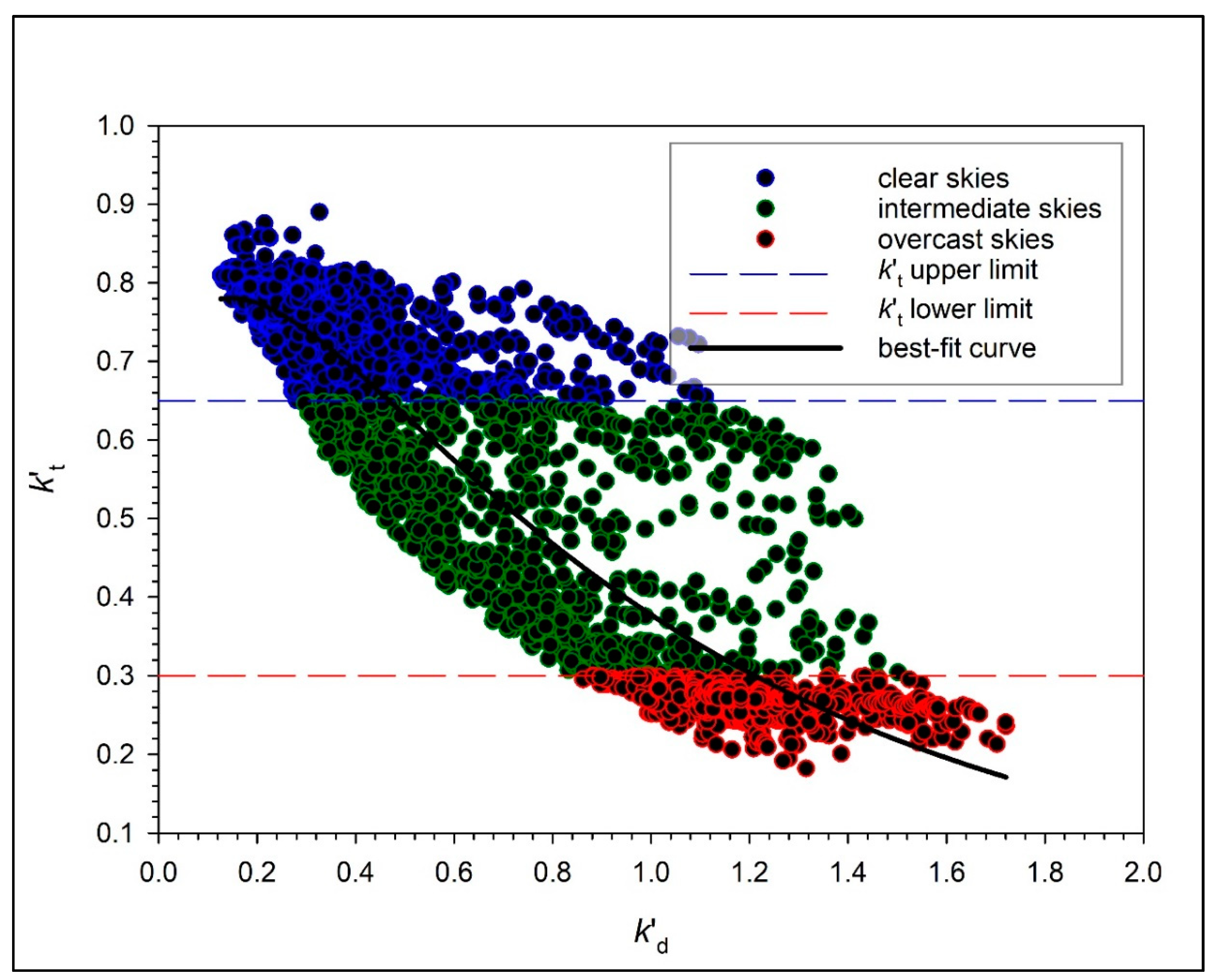
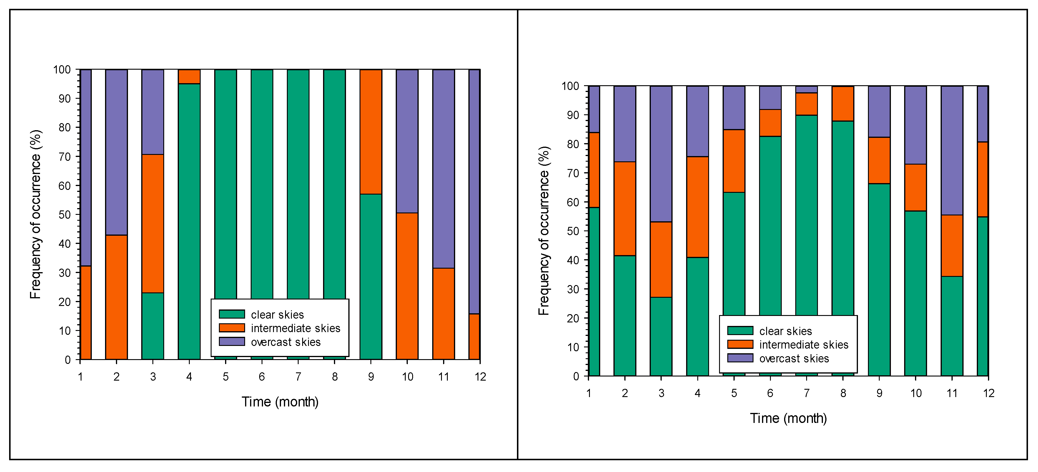
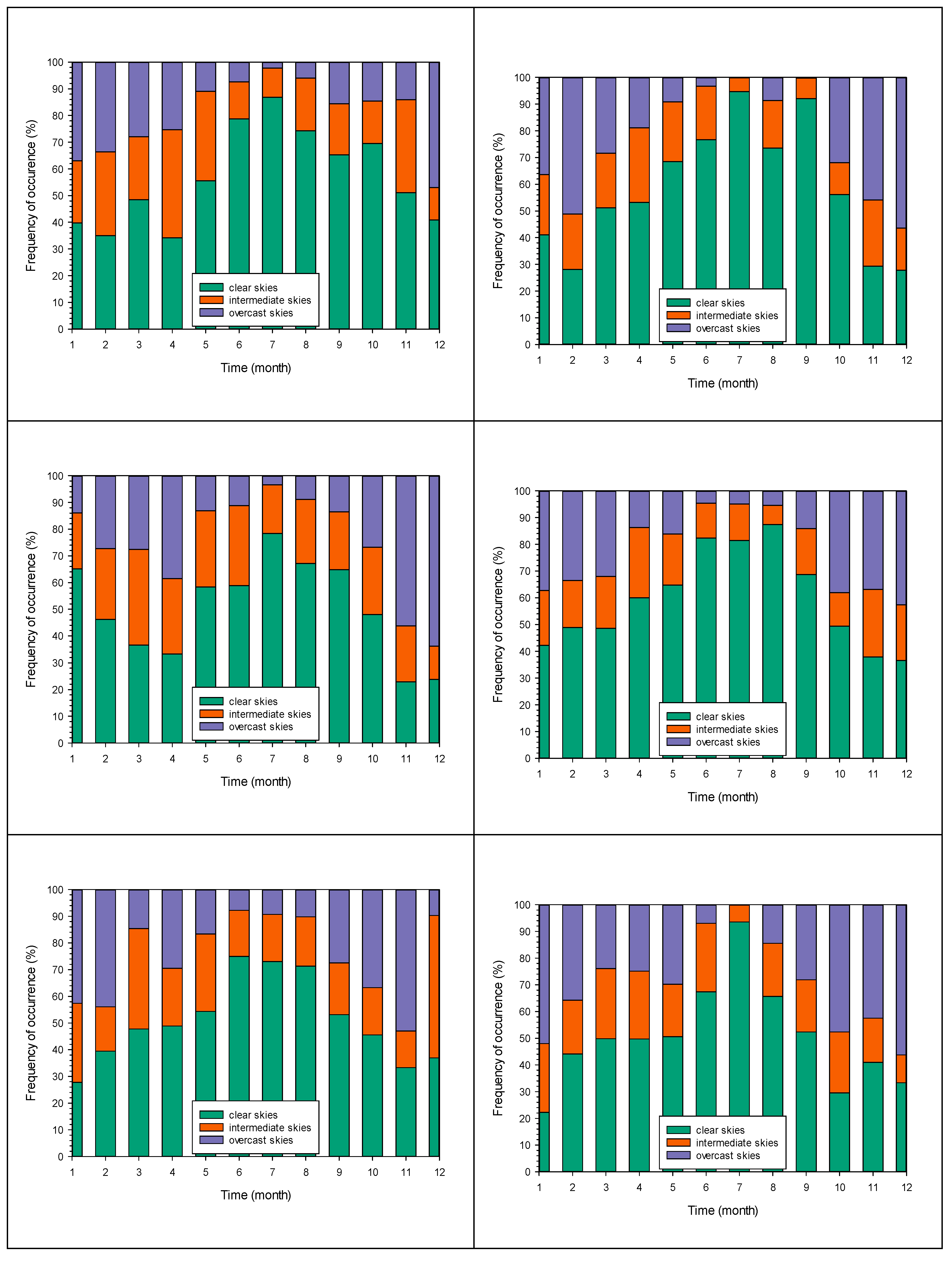
2.1.3. Classification of the Sky Conditions

Kambezidis [47] gives an account of ten possible ways to identify clear skies from available meteorological and/or solar radiation measurements. Nevertheless, he states that the most-adopted technique is the clearness index, k_t, which is defined as the ratio G_e/G_e,extra.sinγ. As regards this index, Reindl et al. [48] have proposed values of k_t > 0.6 and k_t < 0.2 for clear and cloudy skies, respectively. Li and Lam [49] and Li et al. [50] used values of 0 < k_t ≤ 0.15, 0.15 < k_t ≤ 0.7 and k_t > 0.7 for overcast, intermediate and clear skies, respectively, in Hong Kong. Kuye and Jagtap [51] used k_t > 0.65 and 0.12 ≤ k_t ≤ 0.35 for very clear and cloudy skies, respectively, to classify the sky conditions at Port Harcourt, Nigeria. As k_t depends on m, Perez et al. [52] have defined a modified clearness index, k’_t, independent of the air mass:

$${k^{\prime }}_t=\frac{k_t}{0.1+1.031\cdot exp\hspace{0.17em}\left[-1.4/\left(0.9+\frac{9.4}{m}\right)\right]}$$

(18)

This work adopts the modified k_t using the following limits: 0 < k’_t ≤ 0.3, 0.3 < k’_t ≤ 0.65, and 0.65 < k’_t ≤ 1 for overcast, intermediate and clear skies, respectively.

Another index defining the sky conditions is the diffuse fraction, k_d (e.g., [53,54,55,56]), which is the ratio D_e/G_e. This sky-condition parameter also depends on air mass through the solar radiation components. To avoid this dependency, the present work defines a modified diffuse fraction, k’_d, for the first time worldwide, following the formulation of k’_t in Equation (18):

$${k^{\prime }}_d=\frac{k_d}{0.1+1.031\cdot exp\hspace{0.17em}\left[-1.4/\left(0.9+\frac{9.4}{m}\right)\right]}$$

(19)

Figure 1 shows an example of the variation of k’_t vs. k’_d for the site of Alexandroupoli (see

Table 2. List of the meteorological HNMS stations used in this work. WMO: World Meteorological Organization.

Station	Station Name (Region)	Station’s WMO Code (16xxx)	φ (Deg. N)	λ (Deg. E)	Climatic Zone	z (M amsl)
1	Serres (Central Macedonia)	606	41.083	23.567	D	34.5
2	Kastoria (Western Macedonia)	614	40.450	21.283	D	660.9
3	Mikra (outskirts of Thessaloniki, Central Macedonia)	622	40.517	22.967	C	4.8
4	Alexandroupoli (Eastern Macedonia and Thrace)	627	40.850	25.933	C	3.5
5	Kozani (Western Macedonia)	632	40.283	21.783	D	625.0
6	Kerkyra (known as Corfu, Ionian Islands)	641	39.617	19.917	A	4.0
7	Ioannina (Epirus)	642	39.700	20.817	C	484.0
8	Larisa (Thessaly)	648	39.650	22.450	C	73.6
9	Limnos (Northern Aegean)	650	39.917	25.233	B	4.6
10	Anchialos (Thessaly)	665	39.217	22.800	B	15.3
11	Lesvos (Northern Aegean)	667	39.067	26.600	B	4.8
12	Agrinio (Western Greece)	672	38.617	21.383	B	25.0
13	Lamia (Sterea Ellada)	675	38.850	22.400	B	17.4
14	Andravida (Western Greece)	682	37.917	21.283	B	15.1
15	Skyros (Sterea Ellada)	684	38.900	24.550	B	17.9
16	Araxos (Western Greece)	687	38.133	21.417	B	11.7
17	Tanagra (Sterea Ellada)	699	38.317	23.550	A	139.0
18	Chios (Northern Aegean)	706	38.350	26.150	B	4.0
19	Tripoli (Peloponnese)	710	37.533	22.400	C	652.0
20	Elliniko (Attica)	716	37.900	23.750	B	15.0
21	Zakynthos (known as Zante, Ionian Islands)	719	37.783	20.900	A	7.9
22	Samos (Northern Aegean)	723	37.700	26.917	A	7.3
23	Kalamata (Peloponnese)	726	37.067	22.000	A	11.1
24	Naxos (Southern Aegean)	732	37.100	25.533	A	9.8
25	Methoni (Peloponnese)	734	36.833	21.700	A	52.4
26	Spata (Attica)	741	37.967	23.917	B	67.0
27	Kythira (Attica)	743	36.133	23.017	A	166.8
28	Thira (Southern Aegean)	744	36.417	25.433	A	36.5
29	Souda (Crete)	746	35.550	24.117	A	140.0
30	Rodos (known as Rhodes, Southern Aegean)	749	36.400	28.117	A	11.5
31	Irakleio (also written as Heraklion, Crete)	754	35.333	25.183	A	39.3
32	Siteia (Crete)	757	35.120	26.100	A	115.6
33	Kasteli (Crete)	760	35.120	25.333	A	335.0

The names of the stations in the second column are presented as Latin characters, adapted from the Greek alphabet according to the ELOT 743 standard [63], which is based on the ISO 843 [64] standard.

for site information). It is seen that the dependence of k’_t on k’_d has an exponential decay shape (Equation (20)) and not a linear one as is the case of the original indices; for example, k_t = 0.860−1.015 k_d in Hijazin [54]. It is worth mentioning that both paradigms of Alexandroupoli and Hijazin refer to hourly values of the clearness index and the diffuse fraction. The best-fit curve to the hourly data points of Alexandroupoli in Figure 1 has the following form:

$${k^{\prime }}_t=1.1430\cdot exp\hspace{0.17em}\left(-1.1030{k^{\prime }}_d\right)\hspace{0.17em}-\hspace{0.17em}0.4346\cdot exp\hspace{0.17em}\left(-5.5970{k^{\prime }}_d\right)$$

(20)

Expressions of k’_t vs. k’_d for seven other sites have also been derived (see Section 3.3). Further, the characterization of the sky conditions by using k’_d alone, as done with k’_t, is risky, because k’_d depends also upon D_e, which is not always measured in the same manner as G_e. However, the derivation of a relationship of the form k’_d = f(k’_t) may be useful as it can provide information about D_e, if G_e measurements are available in a location.

Figure 2 provides information about the distribution of clear, intermediate and overcast skies over eight sites in Greece following the k’_t limitations. The other sites in Table 2 show similar patterns (not shown here).

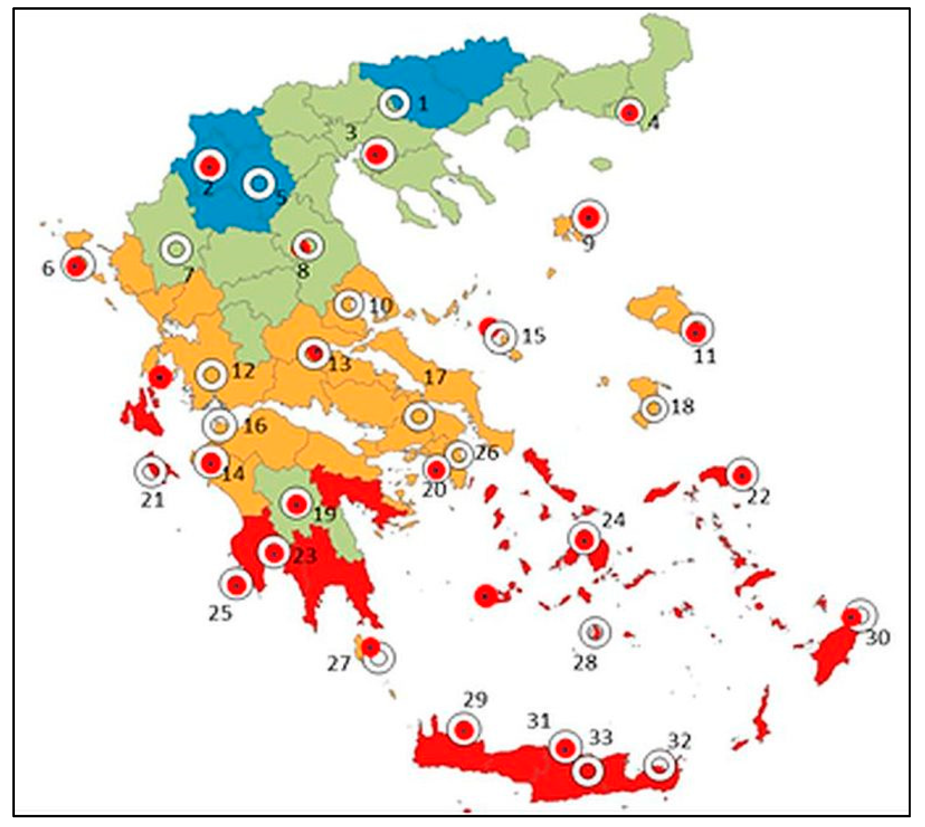
2.2. Data Collection

Under the auspices of the KRIPIS-THESPIA-II project – funded by the General Secretariat of Research and Technology of Greece, the Atmospheric Research Team of the National Observatory of Athens derived TMYs (Typical Meteorological Years) for 33 locations across Greece. A TMY is a complete year of data consisting of hourly or daily values of meteorological and/or radiometric parameters; each TMM (Typical Meteorological Month) of the TMY is chosen via a specific statistical procedure for that month, which is closer to the long-term climatic characteristics of the site for that month. The generation of a TMY is implemented from a database containing the selected parameters in a span of years—usually 15–20 and most preferably 30 years. More details about the generation of the TMYs for Greece are given in Kambezidis et al. [57], where data of meteorological parameters were obtained from 33 HNMS (Hellenic National Meteorological Service) stations during the period 1985–2014 (30 years; see Table 2). For each of the 33 sites, five different TMYs were derived for equal applications; i.e., TMY-Meteorology-Climatology (TMY-MC), TMY-Bio-Meteorology (TMY-BM), TMY-Agro-Meteorology-Hydrology (TMY-AMH), TMY-Energy Design for Buildings (TMY-EDB), and TMY-Photovoltaics (TMY-PV). Each type of TMY contains the necessary meteorological and/or solar radiation parameters. The solar radiation (G_e, B_e, D_e) values for the purpose of TMY generation at each of the 33 stations were derived from the available meteorological data (ambient temperature, relative humidity, atmospheric pressure, sunshine duration) via the MRM (Meteorological Radiation Model; see [58,59,60,61]), because the HNMS stations do not measure solar radiation. Each of those TMYs consists of hourly values of the parameters considered. For the purpose of this work, the databases of the TMYs-PV at the 33 sites have been selected because the climatology of the atmospheric turbidity is more related to solar radiation/energy applications. Table 2 gives the geographical coordinates, climatic zones and altitudes of the 33 stations, while Figure 3 shows their location on the map of Greece. This map also shows the four climatic zones of the country for energy applications [62]. The delimitation of these zones has been based on three parameters: the heating degree days (HDD), the cooling degree hours (CDH) and the available SSR (surface solar radiation) in a region.

Table 3. Range of annual heating degree days (HDD), cooling degree hours (CDH) and available SSR (surface solar radiation) values to define the climatic zones in Greece for energy saving in buildings [61]. The calculation of HDD and CDH considers the following cold and warm periods of the year: (i) climatic zones A, B: 1 November–15 April and 15 May–15 September, respectively, (ii) climatic zones C, D: 15 October–30 April and 1 June–31 August, respectively.

Climatic Zone	HDD (Dimensionless)	CDH (Dimensionless)	SSR (kWh m−2 y−1)
A	<1000	[1300, 4500]	[1700, 1900]
B	[1000, 1500]	[2200, 5500]	[1500, 1700]
C	[1500, 2000]	[1200, 3800]	[1450, 1600]
D	≥2000	≤1500	≤1500

shows the range of those parameters for each climatic zone.

The difference in handling the sites in this work and that in Kambezidis et al. [57] is that Serres has been classified here in the climatic zone D. The reason is that this site is exactly on the border of two zones (C and D, see map in Figure 3); Kambezidis el. [57] considered it in zone C.

2.3. Data Processing

Each TMY-PV at any of the 33 sites in Greece consists of hourly values of ambient temperature (in °C), relative humidity (in %), and global horizontal and direct horizontal solar radiations (in Wm⁻²). As no atmospheric pressure data were included in the TMYs-PV, this parameter was adopted from the corresponding TMYs-MC. All of the above parameters refer to the station’s altitude and have gone through quality-control testing during the generation process of the TMYs (see [57]).

The original SUNAE (Sun’s Azimuth and Elevation) routine, first introduced by Walraven [66], together with its modifications [67,68,69,70] was applied to the geographical coordinates of the 33 stations at every 30 min past the hour for a complete year. To derive the hourly values of the solar altitude, γ, needed for the calculation of m at every site for a complete year, the SUNAE algorithm was applied to each month of the site’s TMY (for description see [57]). Only values of γ greater than or equal to 5° were considered (to avoid the cosine effect); thus, the corresponding T_L, T_UM, k’_t, and k’_d values were discarded. Another data-quality criterion was the rejection of all T_L, T_UM, k’_t, and k’_d values if G_e or B_e were equal to zero. On the other hand, the distinction of skies into overcast, intermediate and clear for the purposes of this work has been based on the criteria mentioned in Section 2.1.3. Furthermore, the hourly values of T_L, T_UM have been kept in the ranges given in Section 2.1.1 and Section 2.1.2, respectively.

The derivation of T_L and T_UM at the 33 sites was based on necessary measured or estimated parameters (B_e, P_z for T_L; B_e, RH, T for T_UM); their values have been taken from the available TMY datasets at the 33 locations. Therefore, one could say that the derived T_L and T_UM annual datasets also correspond to a TMY; thus, the notion of a TATY (Typical Atmospheric Turbidity Year) is introduced here.

3. Results

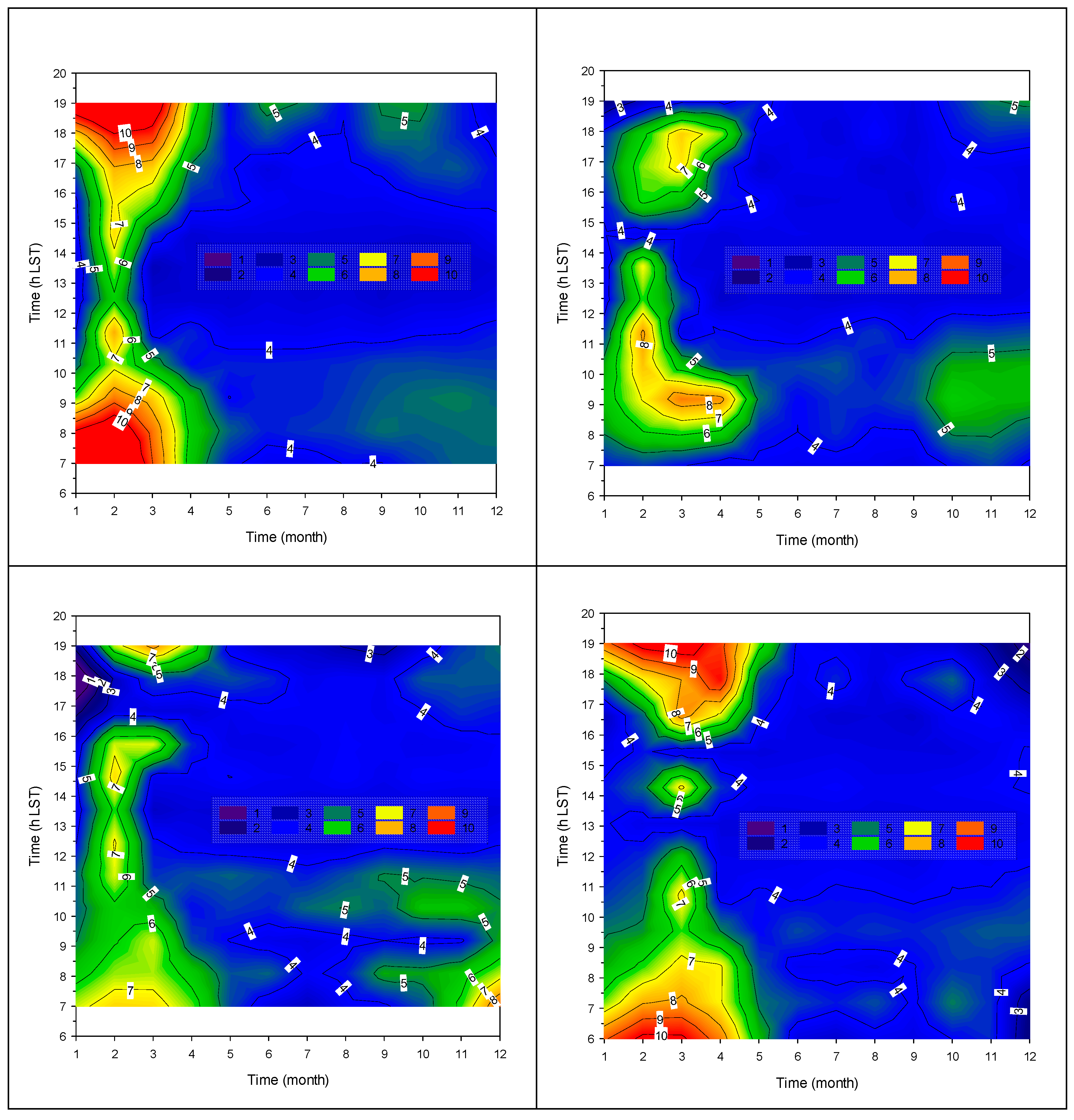
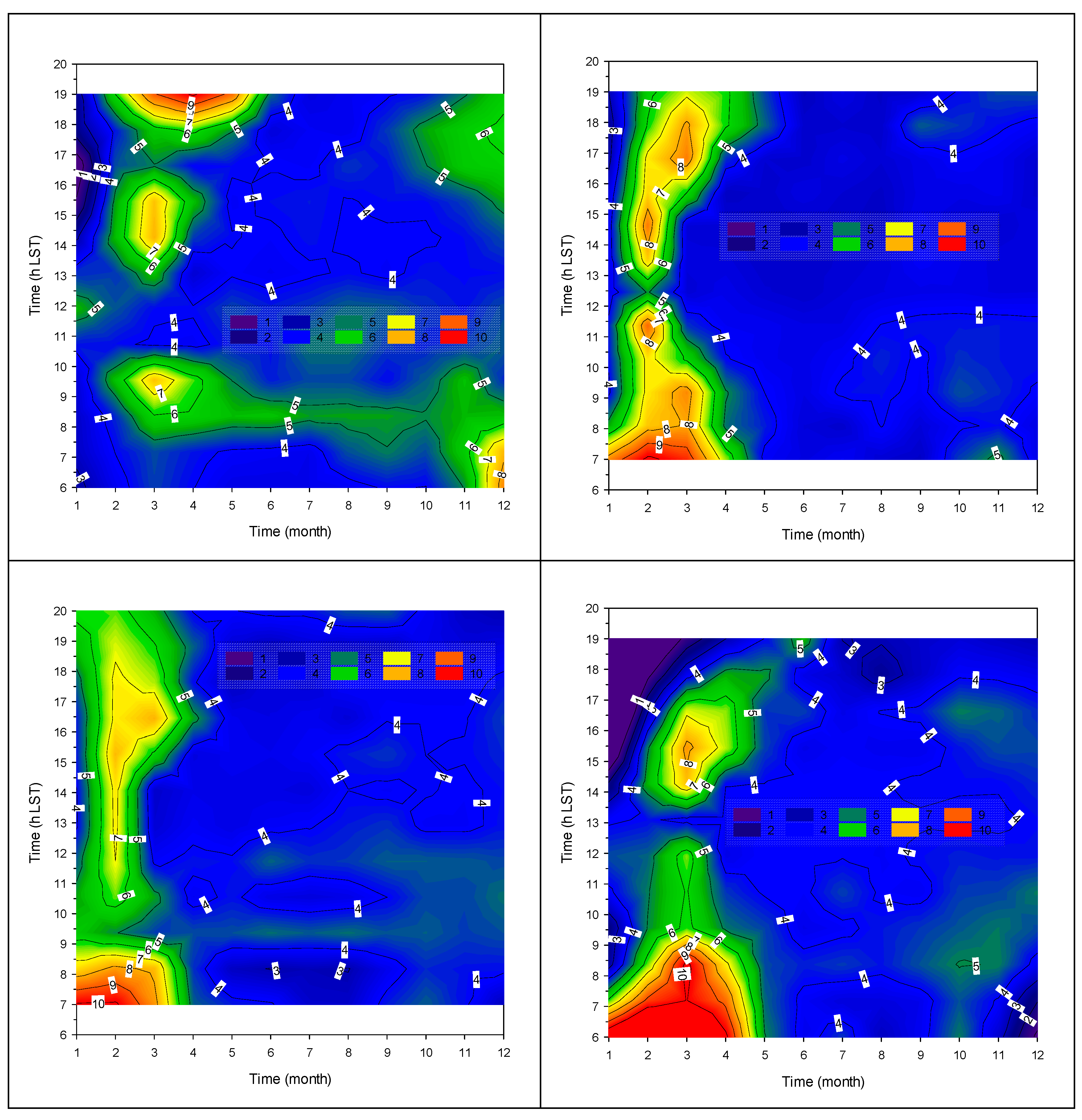
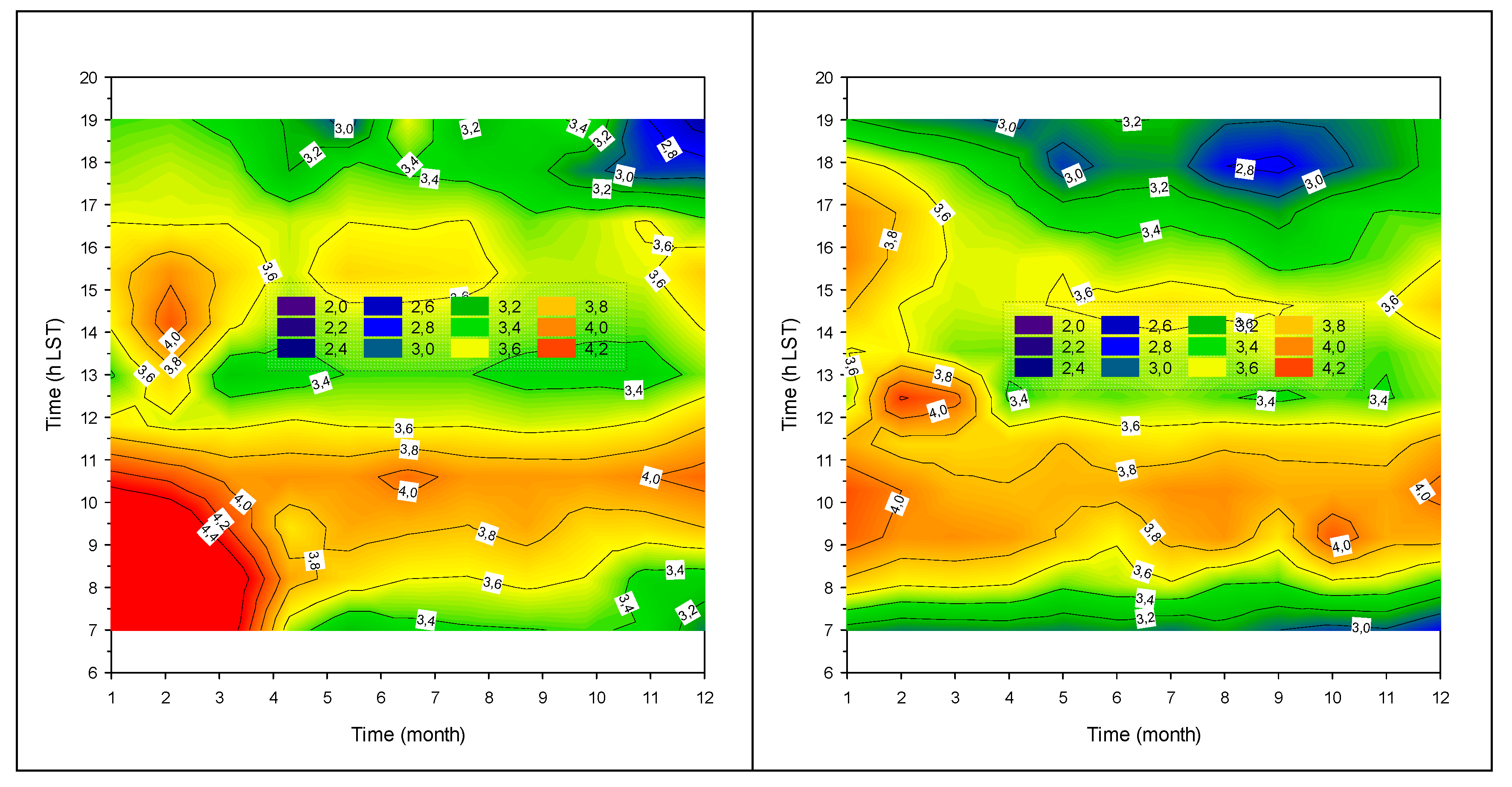
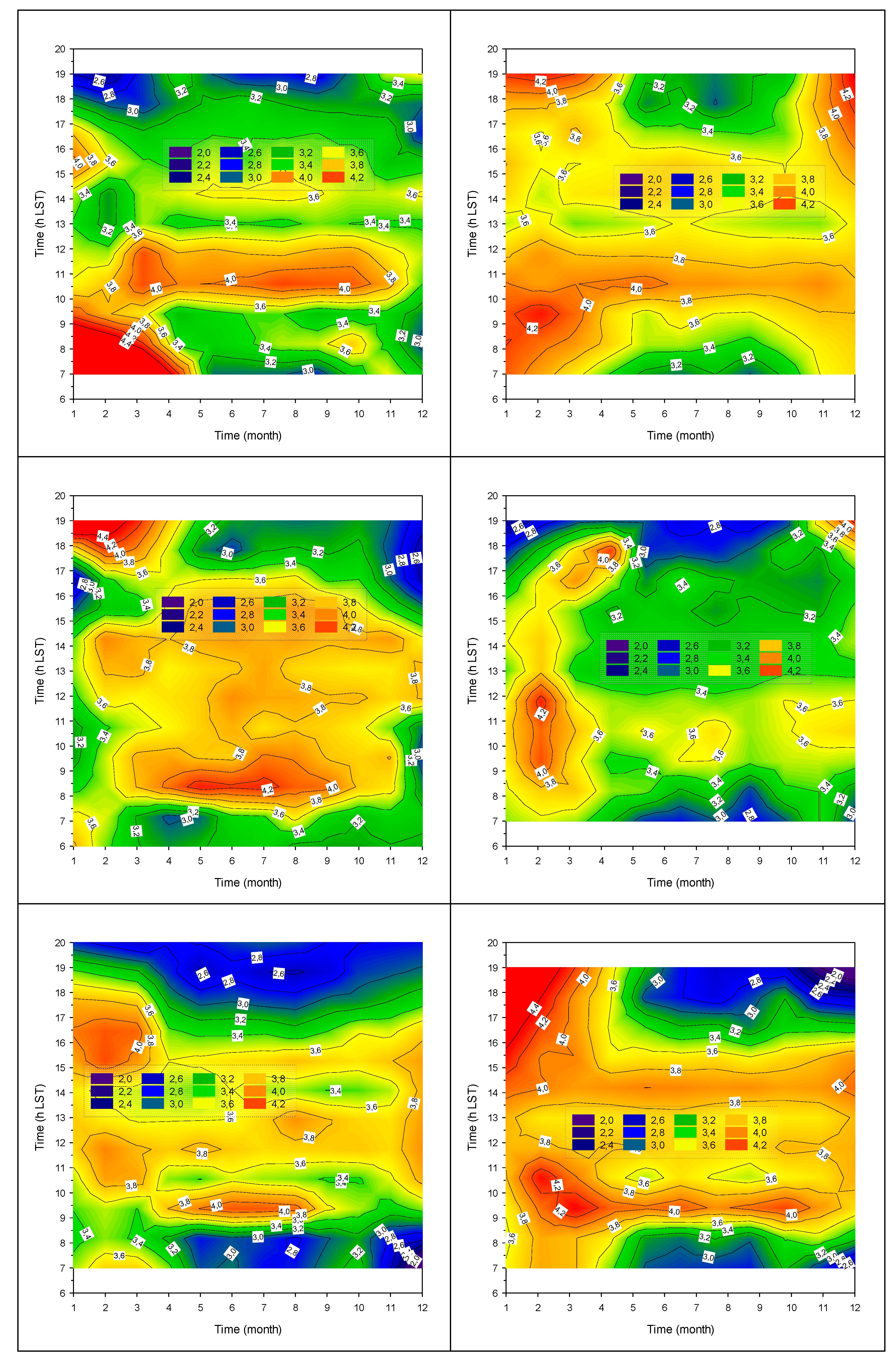
3.1. T_L and T_UM Variation: Month–Hour Diagrams for All-Sky Conditions

Kambezidis et al. [71] first introduced the methodology for the month–hour distribution of a meteorological parameter through its application to daylight levels in Athens. Those researchers listed the advantages of using such an analysis. This methodology is also followed in the present study. Due to the large number of sites considered in this work, it is not possible to show diagrams for all 33 locations; therefore, a pair of representative sites per climatic zone has been chosen (as in Figure 2); these are Irakleio and Kalamata for zone A, Agrinio and Lesvos for zone B, Alexandroupoli and Tripoli for zone C, and Kastoria and Serres for zone D.

Figure 4 shows the month–hour graphs of T_L under all-sky conditions for the selected sites. A general observation is the relatively high values of T_L during almost all day in January, February, March or even early April. Lower values are observed at midday. The morning and evening peaks (8 a.m. and 5–6 p.m.) may correspond to rush hours as the meteorological data used to calculate T_L comes from HNMS stations mostly situated at airports and/or close to towns. Similar observations to ours have been reported over individual years in Rome and Arcavacata di Rende, Italy [13], various locations in Zimbabwe [16], and over Sfax in Tunisia [18]. In late spring, autumn and winter, T_L decreases in the evening because of its sensitivity to low solar elevation angles (higher air masses).

The observations drawn from Figure 4 may have another explanation. According to the definition of the Linke turbidity factor, during the late autumn–winter period, more clean–dry atmospheres are required to produce the observed attenuation of solar radiation because of extended cloudiness and higher humidity in the atmosphere in relation to those in the spring–early autumn period. Another observation from Figure 4 is that the winter T_L values become lower around noon. This occurs for two further reasons: (i) T_L is inversely proportional to the air mass (or solar elevation angle; see Equation (2)), and it therefore decreases at higher m’ values, and (ii) cloudiness and/or ambient humidity are reduced at midday. Similar patterns have been found at the other 25 sites (not shown here).

Figure 5 is equivalent to Figure 4, but it refers to T_UM. T_UM also depends on 1/m’ as T_L, but it has an additional disadvantage that the dust-laden and dust-free atmospheres (see Equation (9)) contain a specified water-vapor content; i.e., the content that exists in the atmosphere at the time of observation (u_w in Equation (14)). This differentiates its behavior slightly in relation to that of T_L, as T_L refers to a dry atmosphere only. Nevertheless, the T_L and T_UM patterns for the same site look very similar; one might observe that, if the T_L values are divided by 10, the T_UM values are obtained. Kambezidis et al. [24] have come to a similar conclusion. The other 25 sites present very similar T_UM patterns (not shown here).

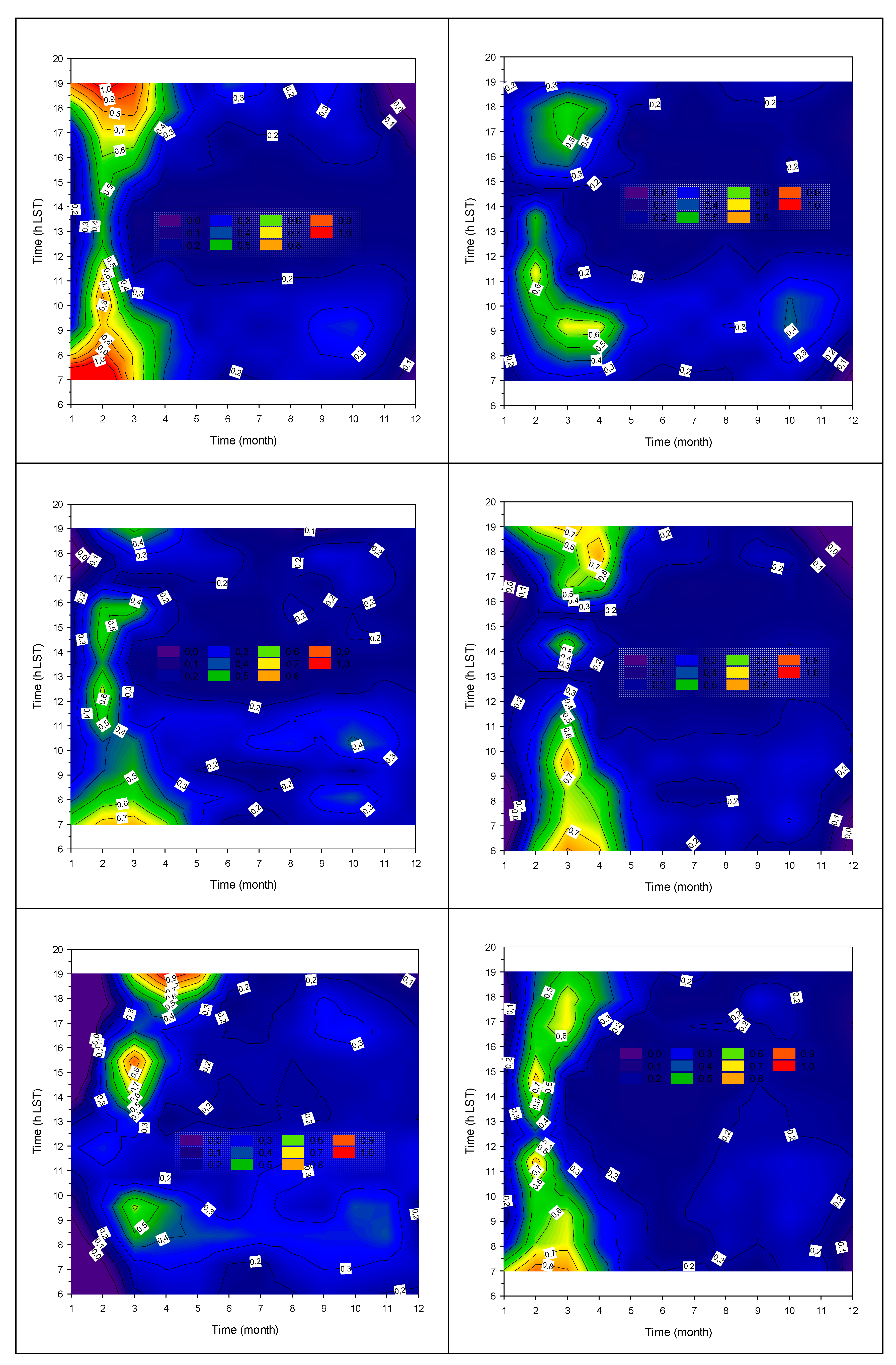
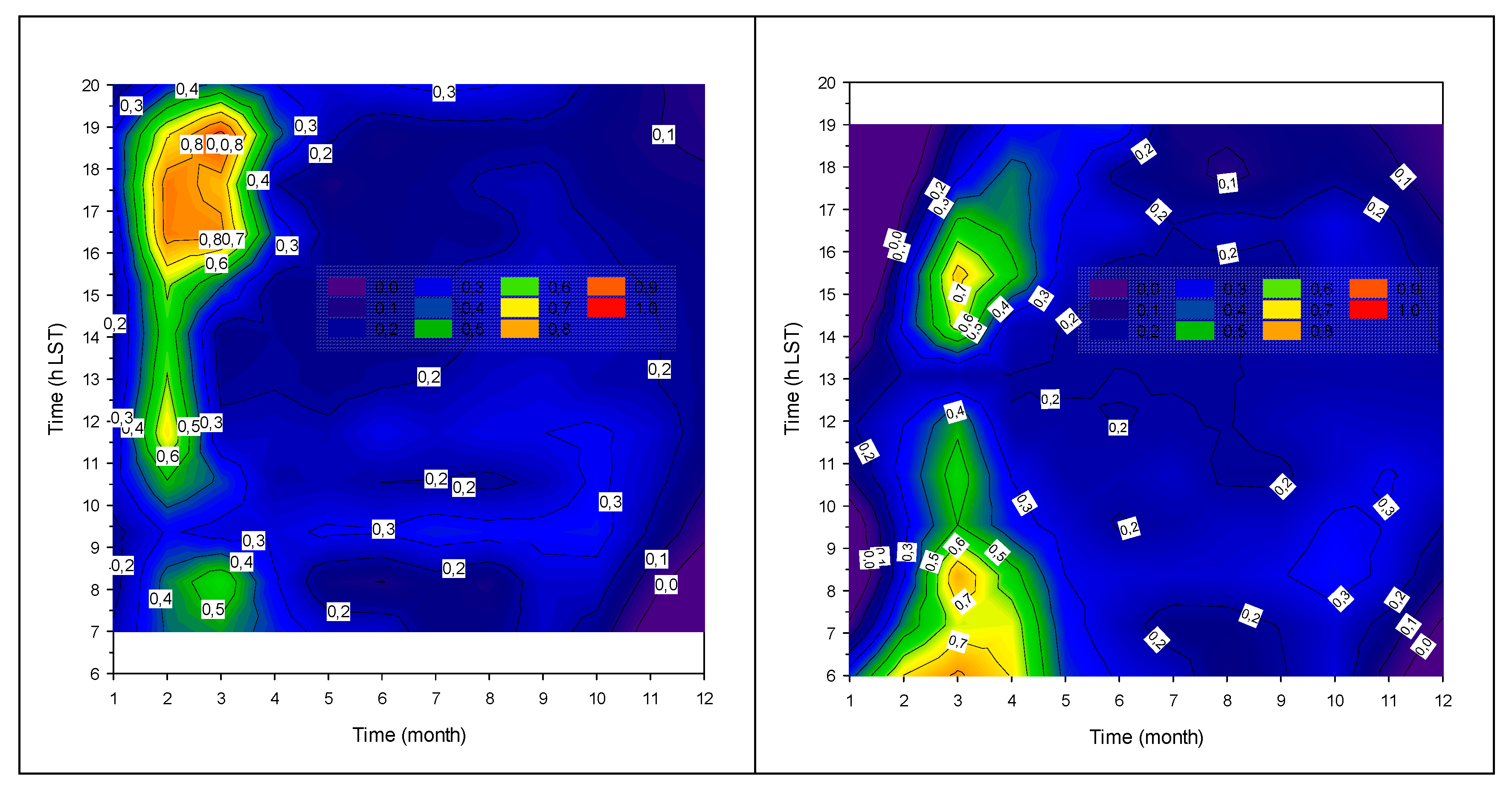
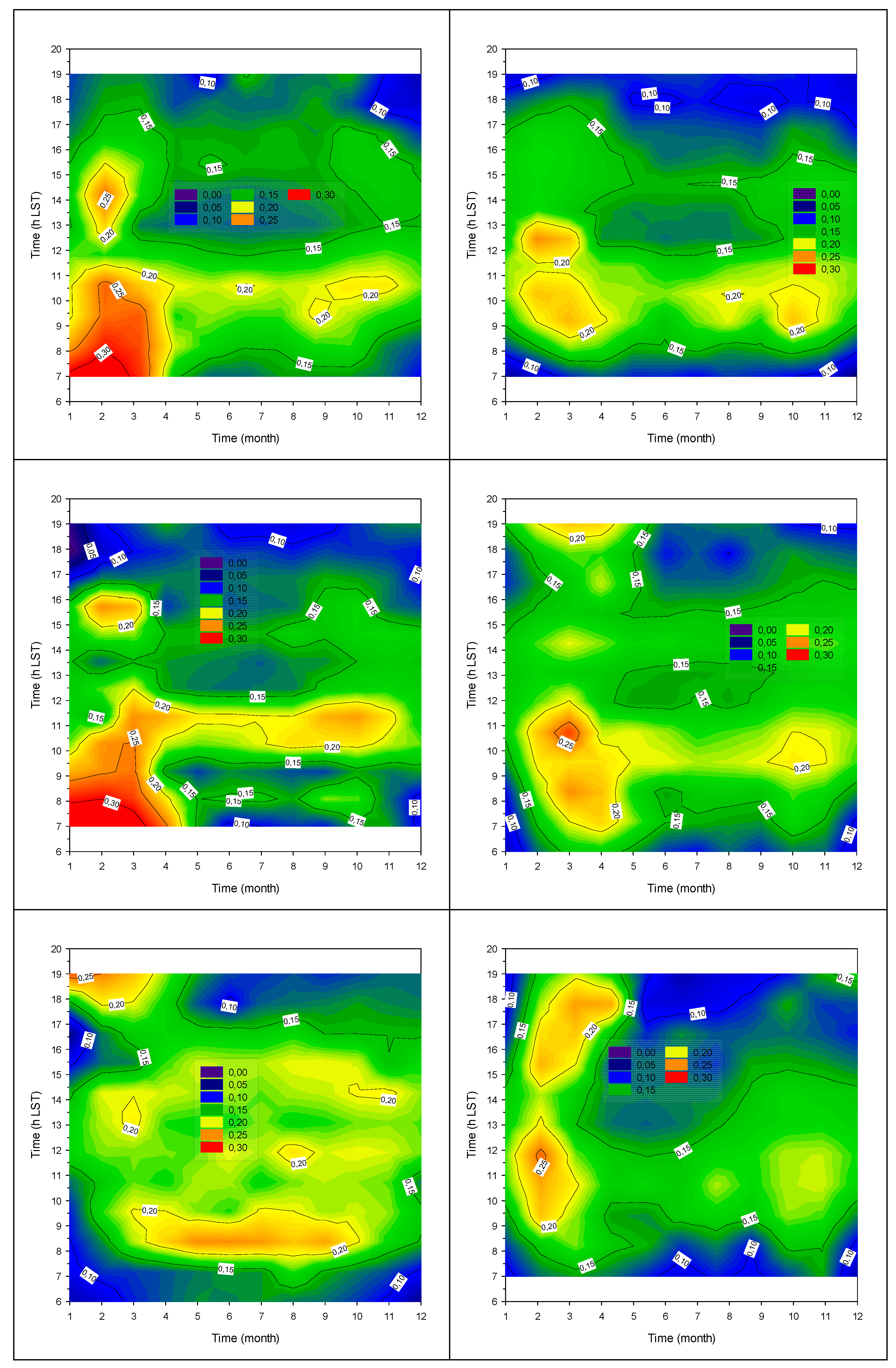
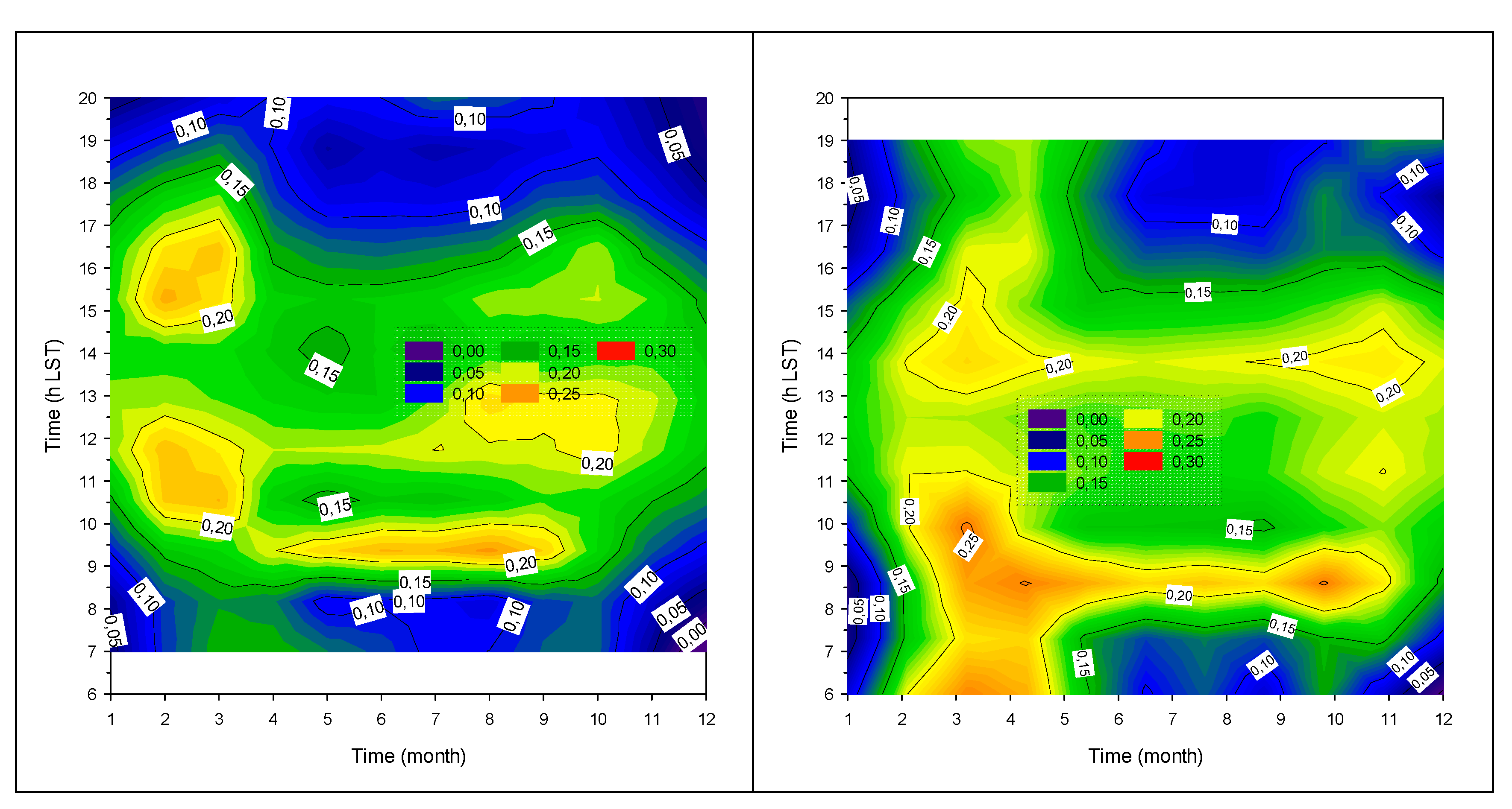
3.2. T_L and T_UM Variation: Month–Hour Diagrams for Clear-Sky Conditions

Figure 6 shows the month–hour graphs of T_L under clear-sky conditions for the selected sites in each climatic zone. In these diagrams, the all-sky T_L patterns seem to be repeated in a clearer way. The morning and evening peaks are retained in the period January–March due to the rush-hour activities. Maximum T_L values are also found in the morning hours throughout the year but are lower than those in late winter–early spring; this occurs because of progressively reduced values of relative humidity. In the evening (late spring–early winter), the T_L values are lower than the morning values for the same reason given for T_L under all-sky conditions. A similar pattern exists for the other 25 sites (not shown here).

The T_UM pattern for clear skies (Figure 7) follows that of T_L as in the case of all-sky conditions. The explanation is the same. Dividing the T_L levels by 10 for any of the eight sites, one almost obtains the T_UM levels for this site, in agreement with Kambezidis et al. [24] for Athens in the period 1975–1984. Similar T_UM patterns for the other 25 sites have been obtained (not shown here).

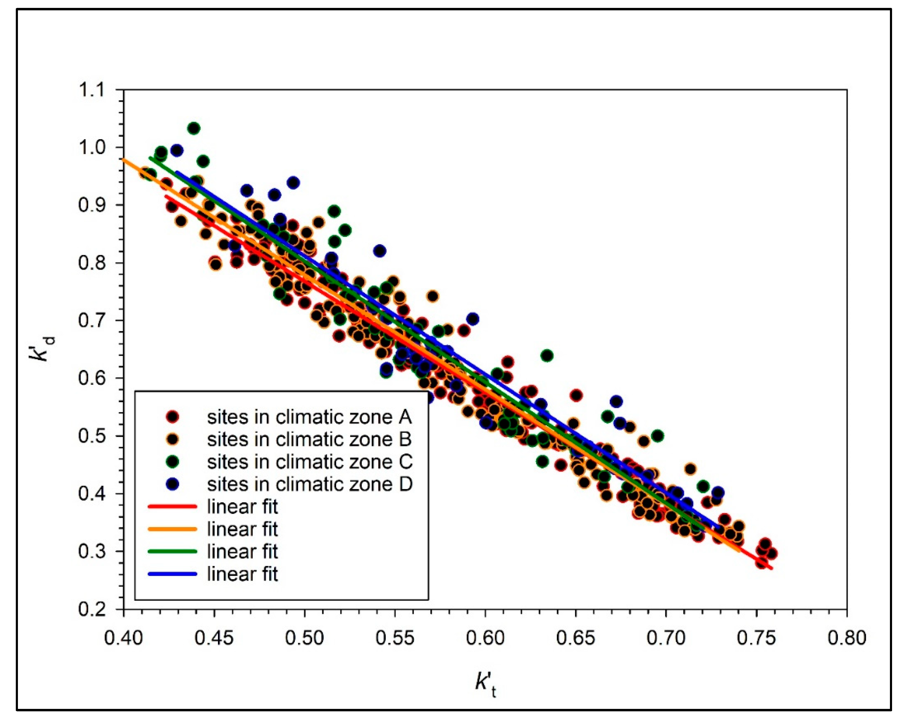
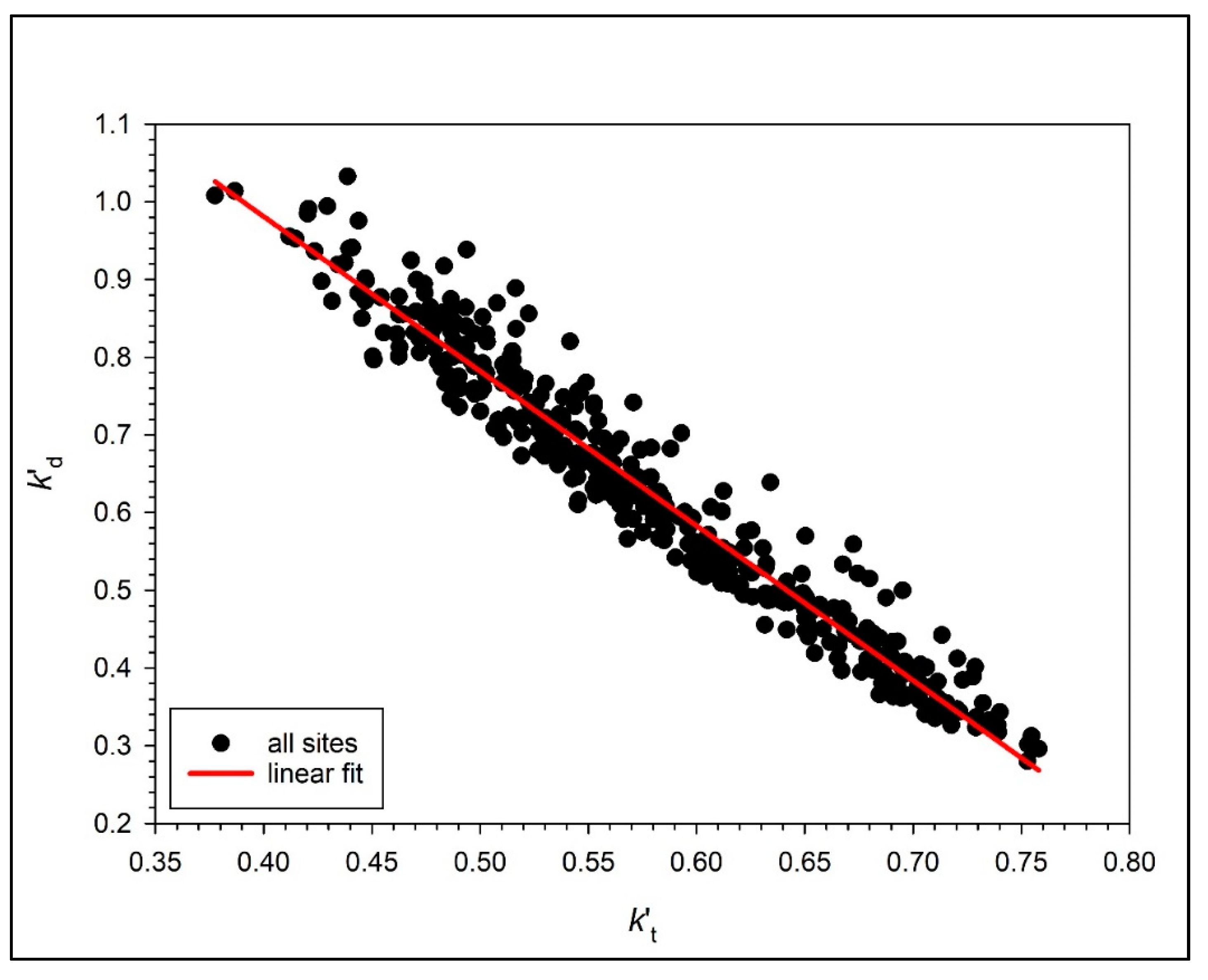
3.3. Variation of k’_d vs. k’_t over Greece

An expression of k’_d as function of k’_t is very useful as D_e can be derived from k’_d provided there are available G_e measurements in a location, as already mentioned in Section 2.1.3. As shown in Figure 1, the hourly values provide a wide dispersion due to extreme weather effects. In order to smooth out any such unwanted effect on the k’_d vs. k’_t relationship, monthly mean values of these indices were considered for the eight selected sites, following the philosophy of the eight representative sites in the four climatic zones of Greece. On the other hand, monthly values are sufficient for engineering applications.

Table 4. Coefficients and R² of the relationship k’_d = a + b k’_t for the eight selected sites in Greece. The relationships have been derived from monthly mean k’_d, k’_t values under all-sky conditions during TATY.

Climatic Zone	Site	a	b	R2
B	Agrinio	1.8616	−2.1402	0.93
C	Alexandroupoli	1.7406	−1.9311	0.92
A	Irakleio	1.7201	−1.9172	0.99
A	Kalamata	1.6518	−1.7932	0.91
D	Kastoria	2.0177	−2.3781	0.94
B	Lesvos	1.7920	−1.9125	0.98
D	Serres	1.8999	−2.1945	0.94
C	Tripoli	1.8737	−2.1123	0.96

provides the coefficients for the linear k’_d vs. k’_t equations under all-sky conditions. On the other hand, by grouping the monthly mean k’_d vs. k’_t data pairs of the stations which belong to the same climatic zone, new best-fit lines were obtained and are shown in Figure 8. It is seen from the linear regression equations that the best-fit lines of the zonal pairs A, B, C, and D are very close to each other. This gives the freedom to derive an equation for all climatic zones (Figure 9).

A corresponding regression analysis of the k’_d vs. k’_t data for clear skies has been carried out for the eight selected sites (not shown here) giving linear regression equations with R² much less than 0.40. This could be anticipated since D_e included in k’_d can vary more than G_e during clear weather depending on the aerosol loading in the atmosphere; on the contrary, during all-sky conditions, D_e is reduced and co-varies with G_e.

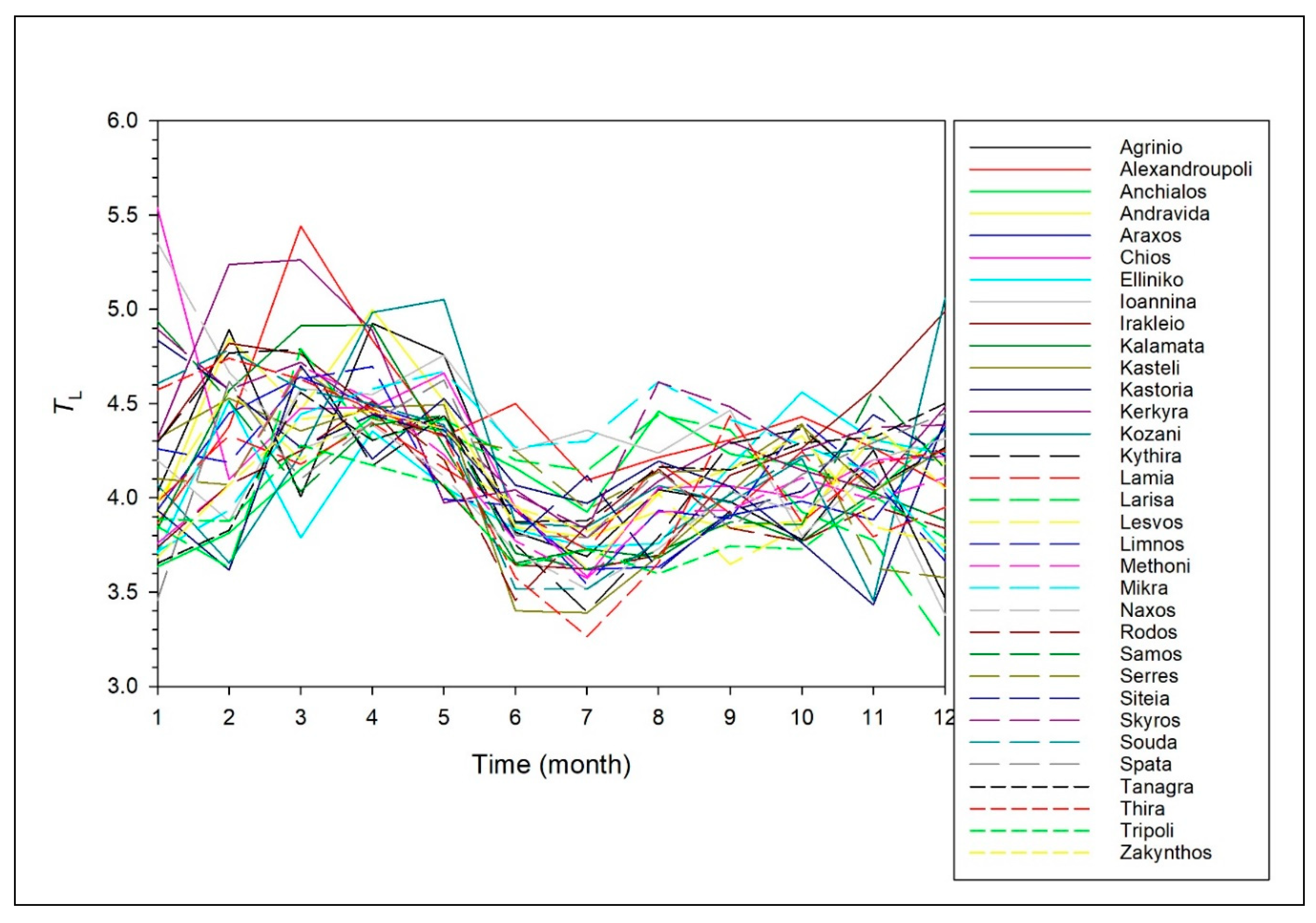
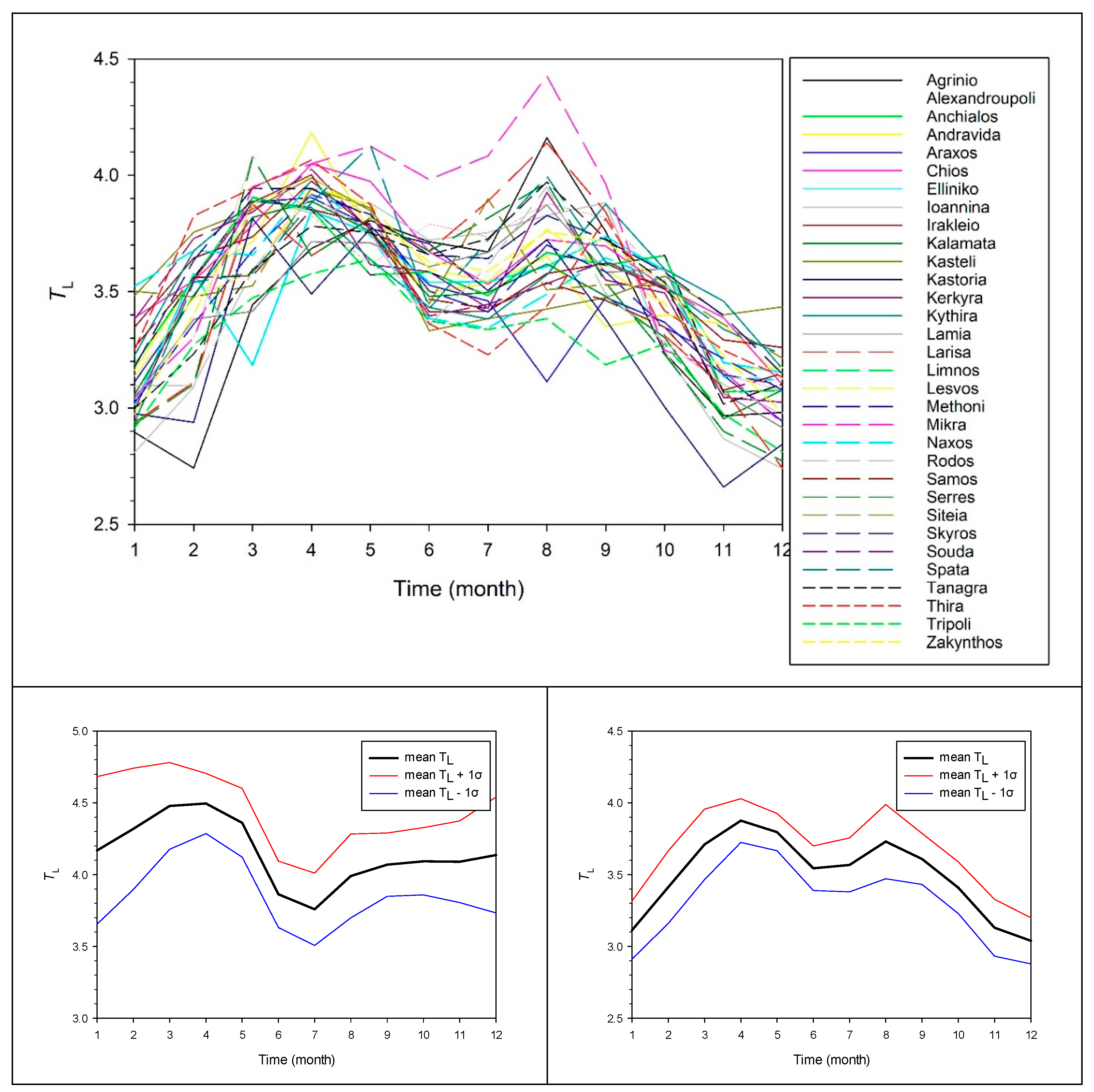
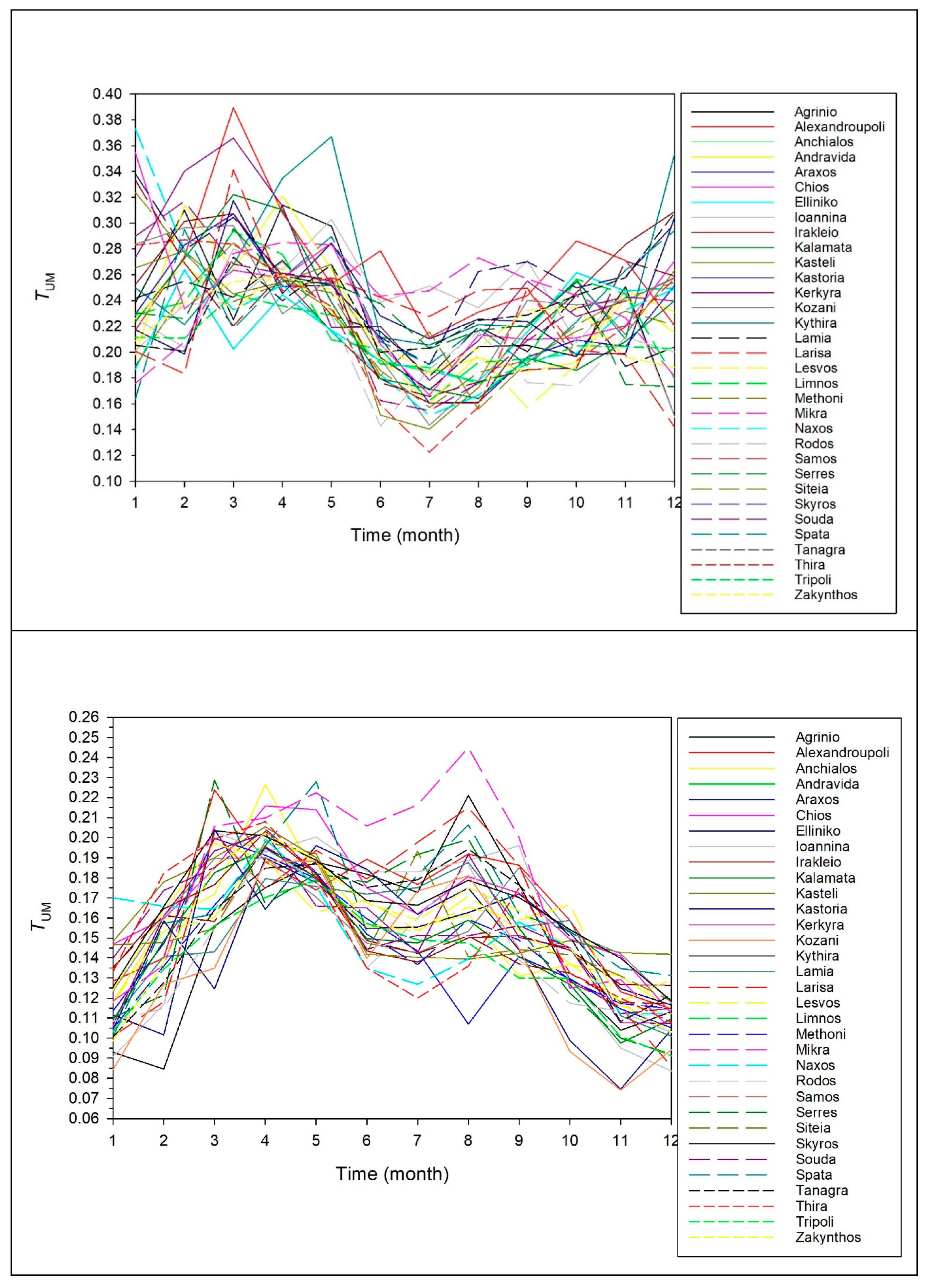
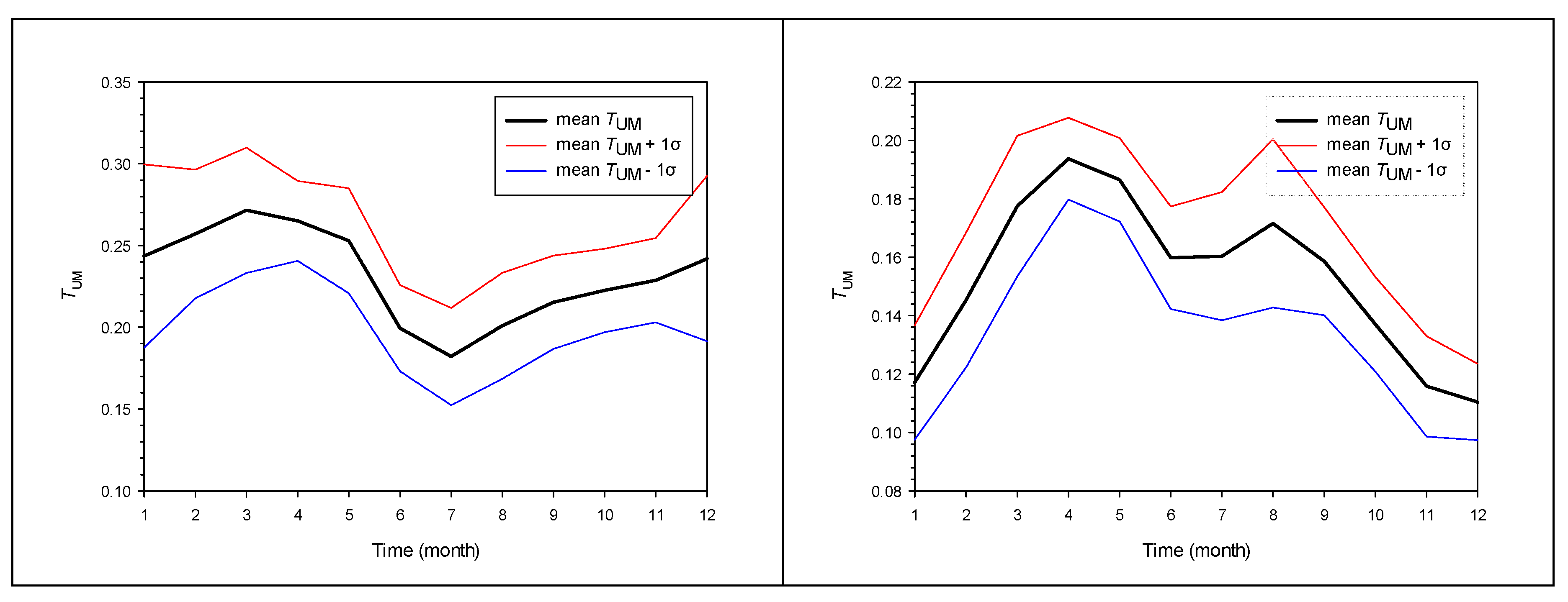
3.4. Intra-Annual Variation of T_L and T_UM

Figure 10 presents the variation of the monthly mean T_L values at all 33 stations under all and clear-sky conditions. The average and ± 1σ (±1 standard deviation) curves are also shown for both types of skies.

It is seen from Figure 10 that T_L obtains a peak in March–April and shows a rather flat behavior after September for all-sky conditions (lower left graph). The black curve is the average of all 33 T_L variations. Similar behavior is shown by the intra-annual variation of T_L under clear skies. There are two pronounced peaks in April and August (lower right graph). Very similar intra-annual patterns and magnitudes of T_L were reported by Pedrόs et al. [72] for Valencia, Spain; by El-Wakil et al. [73] for Cairo, Egypt; by Diabate et al. [14] for several sites in Africa; and by Eftimie [74] (2009) for Braşov, Romania. The spring and autumn peaks may be due to the frequent wind streams from Northern Africa, which may bring desert dust over Greece. The Sahara-dust transport has been a rather frequent phenomenon in the recent 20 years [75]. On the other hand, the summer minimum may be attributed to the strong cleansing northeasterly winds (called Etesians), which make the atmosphere drier. Figure 11 is same as Figure 10, but it refers to T_UM. The peaks and the low summer values here have a similar interpretation to that given for T_L.

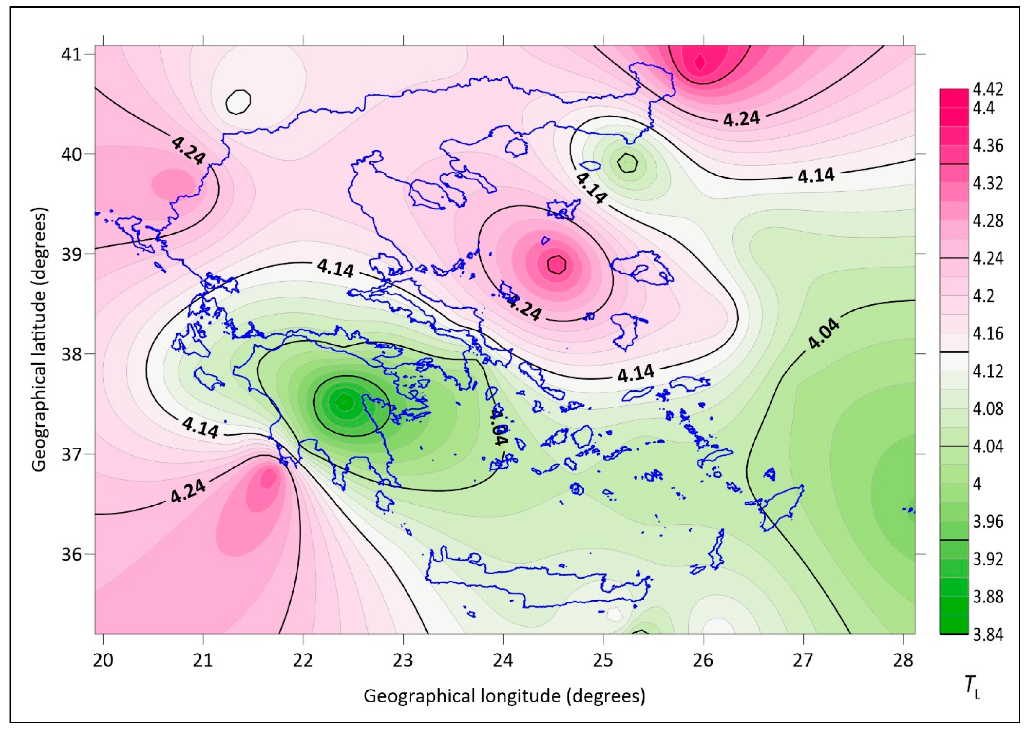
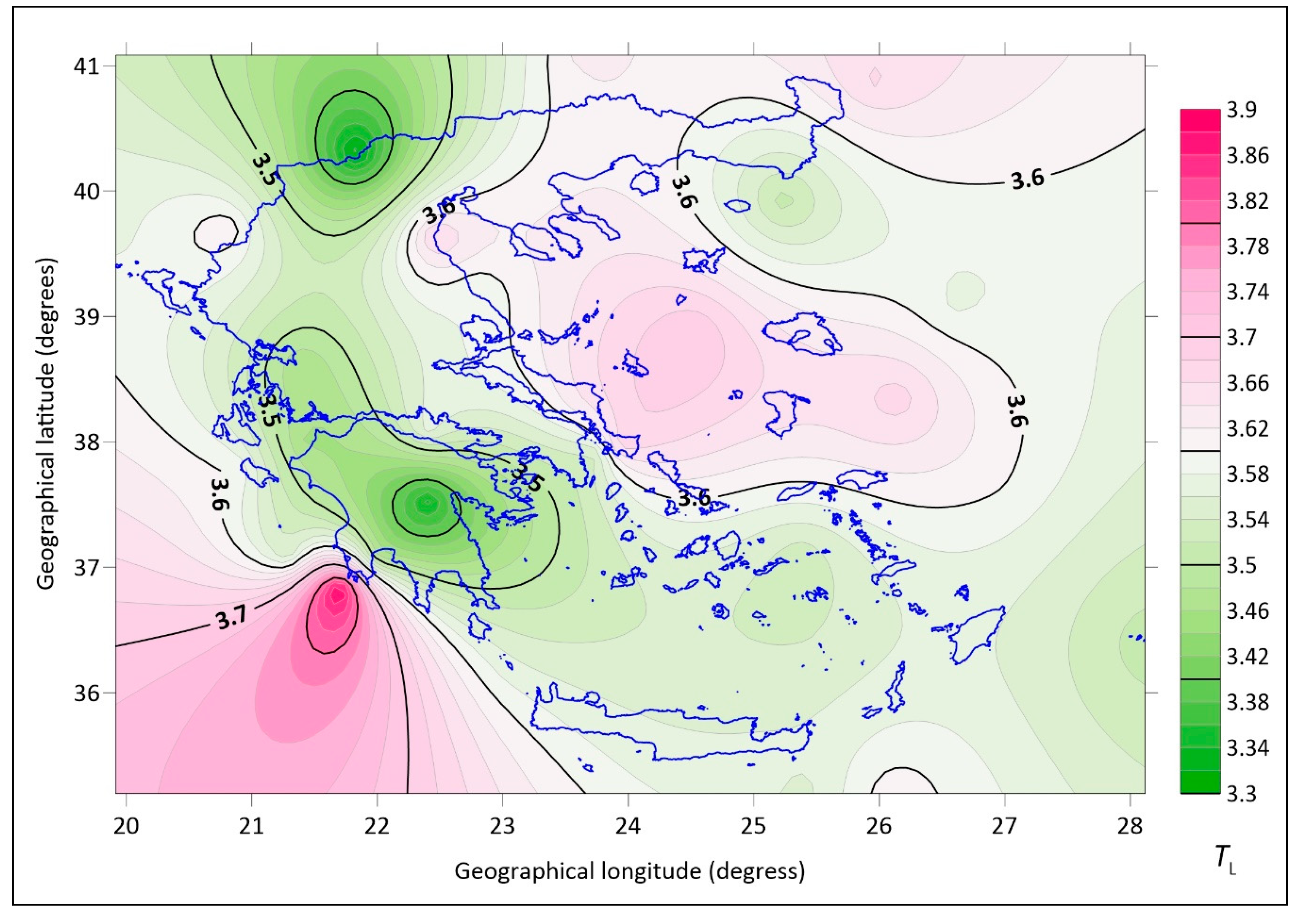
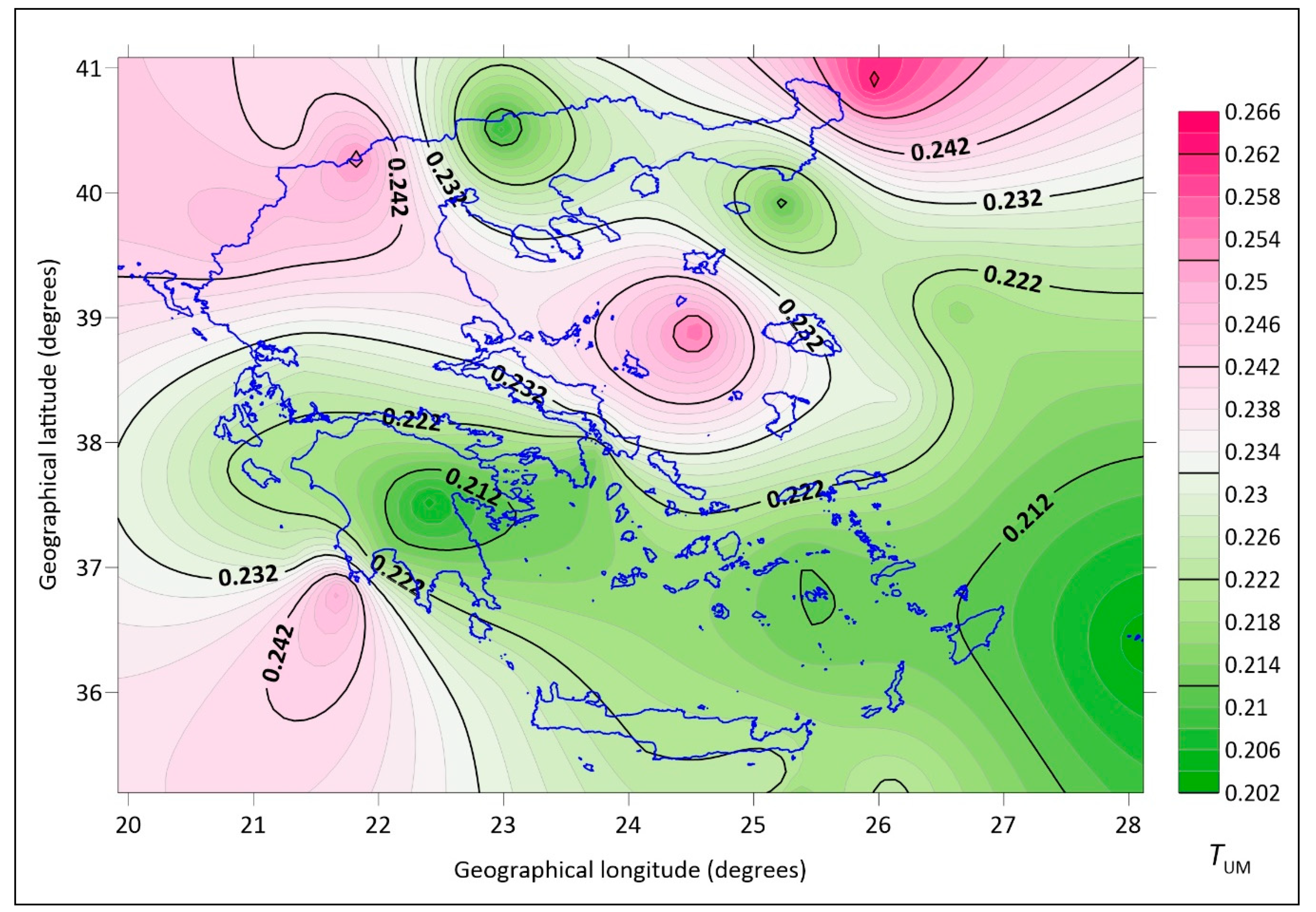
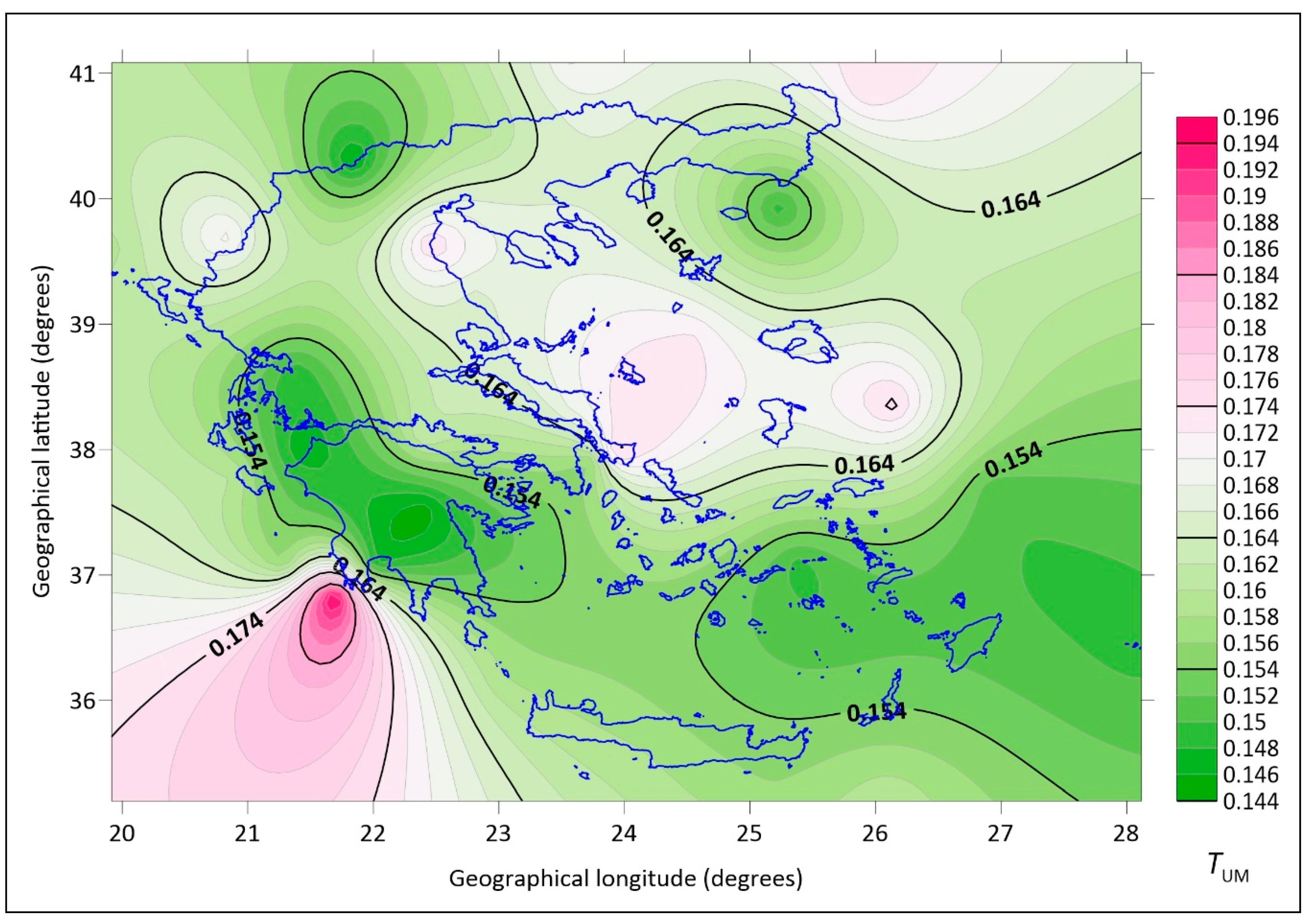
3.5. Maps of Annual Mean T_L and T_UM

Figure 12 and Figure 13 present the distribution of the annual mean values of T_L and T_UM over the Greek territory, respectively, for all and clear-sky conditions. Two major peaks are seen in both T_L and T_UM values for all skies; one is centered over the South Ionian Sea and the other over the Central Aegean Sea. Both peaks are located in a northeast–southwest direction, and it is believed they are due to Sahara-dust transport mostly over Southern Greece in spring, late summer, and early autumn (first peak) and the turbulent air during high northeasterly winds over the Aegean Sea almost all-year round (second peak). During clear-sky conditions, the second peak is drastically reduced because it is related to the Etesian winds that blow during summertime and are associated with minimum humidity in the atmosphere.

As far as the minima in the T_L and T_UM annual values are concerned, these are spotted over Peloponnese (T_L) or extended to the South Aegean Sea (T_UM). These broad minima may be thought as a dividing line between high-pressure cells over the Aegean and low-pressure cells in the Southern Ionian Sea.

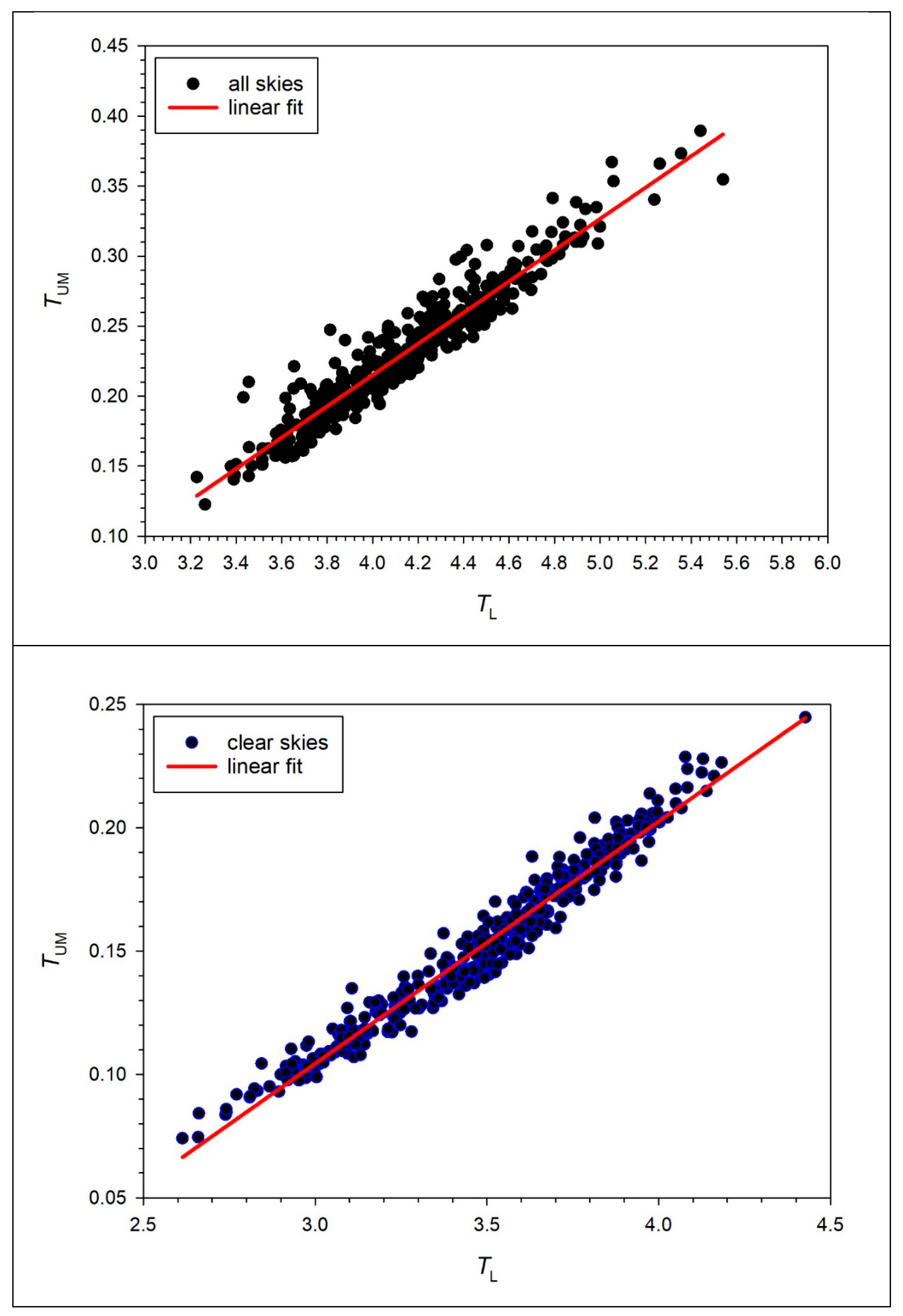
3.6. Variation of T_UM vs. T_L over Greece

There are few studies worldwide that deal with the Unsworth–Monteith turbidity coefficient because of its dependence on the water-vapor content in the atmosphere, as stated in Section 3.1. However, those that exist show a straightforward linear dependence of T_UM on T_L and vice versa. Figure 14 shows this dependence for all and clear-sky conditions over Greece.

Kambezidis et al. [24] provided the relationship T_UM = −0.11 + 0.07 T_L, R² = 0.88 for Athens in the period 1975–1984. Furthermore, Kambezidis et al. [25] provided the expression T_UMvis = −0.1338 + 0.1360 T_Lvis, R² = 0.99 for Athens in the period 1992–1995, where vis refers to the visible band of the solar spectrum. In an updated work about the Linke and Unsworth–Montheith turbidity parameters for Athens, Kambezidis et al. [26] provided the relationship T_UM = −0.1690 + 0.0939 T_L, R² = 0.97 in the period 1975–1995, while Jacovides et al. [76] derived the expression T_UM = −0.182 + 0.0837 T_L, R² = 0.99 for the same site in the period 1954–1991. It is interesting to note that the coefficients of these equations for Athens are in close agreement with those provided for clear-sky conditions for all climatic zones in Greece (see Figure 14). Pedrόs et al. [72] provided a relationship for T_UM as a function of β for Valencia, Spain in the period 1990–1996 instead of T_L.

4. Conclusions

The present study estimated the Linke (T_L) and Unsworth–Monteith (T_UM) turbidity parameters at 33 sites in Greece under all and clear-sky conditions over a year. That year was considered typical (Typical Atmospheric Turbidity Year, TATY) because the estimation of both turbidity factors was based on values of the meteorological parameters that comprise recently-derived Typical Meteorological Years for the same sites. Each TATY consists of the same TMMs as in the TMYs-PV for the specific location.

The present work presented some innovations: (i) the notion of TATY was introduced for the first time worldwide; (ii) turbidity-parameter maps for Greece were derived for the first time; (iii) the definition of the modified diffuse fraction was introduced for the first time worldwide; and (iv) use of the climatic zones of Greece for energy purposes was made, since atmospheric turbidity is used in advanced solar codes to estimate solar radiation at a location destined for energy applications (e.g., PV installations). For the sake of simplicity, two representative sites per climatic zone were selected in some parts of the analysis.

Month–hour graphs for T_L and T_UM were prepared for the eight selected sites. For all-sky conditions, relatively high values of T_L were found in the mornings and evenings during January–March or even early April; lower values were found in the other months of the year. The T_UM variation indicated a similar pattern to that of T_L with a slight differentiation because of the dependence of T_UM on the water vapor in the atmosphere. Under clear skies, the T_L month–hour graphs showed a pattern resembling the all-sky pattern. The morning and evening peaks were retained in the period January–March, with maximum values in the morning hours throughout the year, but these were lower than those in late winter–early spring. In the evening (late spring–early winter), the T_L values were lower than the morning values. T_UM followed the T_L pattern as in the case of all skies. Similar patterns were found for the other 25 sites, but they were not shown in the study for space-saving reasons.

The intra-annual variation of both parameters showed a pattern with maximum values in early spring and late summer and lower values in summertime and most winter months. This behavior was found to be consistent with the intra-annual variation of the turbidity factors at other sites in Europe and Africa.

Maps of the annual mean values of the turbidity parameters over Greece for all and clear-sky conditions were prepared. Persistent low values were found over Peloponnese all over the year and higher values in the southern part of the Ionian Sea.

Because of the difficulty in estimating T_UM (i.e., more elaborate calculations than for T_L; compare methodologies in Section 2.1.1 and Section 2.1.2), linear expressions with high coefficients of determination (R²) were given for T_UM as function of T_L for all sites and both all and clear-sky conditions.

Finally, an attempt to facilitate the estimation of the diffuse horizontal solar radiation at any location in Greece was made, if the global horizontal radiation is known or can be estimated via a solar code. Linear expressions of k’_d vs. k’_t were derived for the sites in each climatic zone as well as for all sites regardless of zone. The expressions provided high values of R², thus showing their applicability.

References

1. Iqbal, M. An Introduction to Solar Radiation; Academic Press: Toronto, ON, Canada, 1983. [Google Scholar]
2. Ångström, A. On the atmospheric transmission of sun radiation and dust in the air. Georg. Ann. 1929, 2, 156–166. [Google Scholar]
3. Ångström, A. Techniques of determining the turbidity of the atmosphere. Tellus 1961, 13, 214–223. [Google Scholar] [CrossRef] [Green Version]
4. Ångström, A. Parameters of atmospheric turbidity. Tellus 1964, 16, 64–75. [Google Scholar] [CrossRef] [Green Version]
5. Schüepp, W. Die bestimmung der komponenten der atmosphärischen turbung aus aktinometermessungen. Arch. Meteorol. Geophys. Bioklim. 1949, B1, 257–317. [Google Scholar] [CrossRef]
6. Linke, F. Transmissionkoefzient und Trübungsfaktor. Beitr. Phys. Frei Atmos. 1922, 10, 91. [Google Scholar]
7. Linke, F. Messungen der sonnestrahlung beivier freiballonfahrten. Beitr. Phys. Frei Atmos. 1929, 15, 176. [Google Scholar]
8. Unsworth, M.H.; Monteith, J.L. Aerosol and solar radiation in Britain. Q. J. R. Meteorol. Soc. 1972, 98, 778–797. [Google Scholar] [CrossRef]
9. Polavarapu, R.J. Atmospheric turbidity over Canada. J. Appl. Meteorol. 1978, 17, 1368–1374. [Google Scholar] [CrossRef] [Green Version]
10. Abdelrahman, M.A.; Said, A.M.; Shuaib, A.N. Comparison between atmospheric turbidity coefficients of desert and temperate climates. Sol. Energy 1988, 40, 219–225. [Google Scholar] [CrossRef]
11. Grenier, J.C.; de la Casinière, A.; Cabot, T. A spectral model of Linke’s turbidity factor and its experimental implications. Sol. Energy 1994, 52, 303–313. [Google Scholar] [CrossRef]
12. Eaton, F.D.; Hines, J.R.; Drexler, J.J.; Soules, D.B. Short-term variability of atmospheric turbidity and optical turbulence in a desert environment. Theor. Appl. Climatol. 1997, 56, 67–81. [Google Scholar] [CrossRef]
13. Cucumo, M.; Marinalli, V.; Oliveri, G. Experimental data of the Linke turbidity factor and estimates of the Ångström turbidity coefficient for two Italian localities. Renew. Energy 1999, 17, 397–410. [Google Scholar] [CrossRef]
14. Diabate, L.; Remund, J.; Wald, L. Linke turbidity factors for several sites in Africa. Sol. Energy 2003, 75, 111–119. [Google Scholar] [CrossRef] [Green Version]
15. Zakey, A.S.; Abdelwahab, M.M.; Makar, P.A. Atmospheric turbidity over Egypr. Atmos. Environ. 2004, 38, 1579–1591. [Google Scholar] [CrossRef]
16. Hove, T.; Manyumbu, E. Estimates of the Linke turbidity factor over Zimbabwe using ground-measured clear-sky global solar radiation and sunshine records based on a modified ESRA clear-sky approach. Renew. Energy 2013, 52, 190–196. [Google Scholar] [CrossRef]
17. Bilbao, J.; Rόman, R.; Miguel, M. Turbidity coefficients from normal direct solar irradiance in central Spain. Atmos. Res. 2014, 143, 73–84. [Google Scholar] [CrossRef]
18. Saad, M.; Trabelsi, A.; Masmoudi, M.; Alfaro, S.C. Spatial and temporal variability of the atmospheric turbidity in Tunisia. J. Atmos. Solar-Terr. Phys. 2016, 149, 93–99. [Google Scholar] [CrossRef]
19. Ulscka-Kawalkowska, J.; Posyniak, M.; Markowicz, K.; Podgόrski, J. Comparison of the Linke turbidity factor in Warsaw and in Belsk. Bull. Geogr. 2017, 13, 71–81. [Google Scholar] [CrossRef] [Green Version]
20. Mateos, D.; Cachorro, V.E.; Velasco-Merino, C.; O’Neill, N.T.; Burgos, M.A.; Gonzalez, R.; Toledano, C.; Herreras, M.; Calle, A.; de Frutos, A.M. Comparison of three different methodologies for the identification of high atmospheric turbidity episodes. Atmos. Res. 2020, 237, 104835. [Google Scholar] [CrossRef]
21. Karalis, J.D. The turbidity parameters in Athens. Arch. Meteorol. Geophys. Biokl. 1976, 24, 25–34. [Google Scholar] [CrossRef]
22. Katsoulis, B.D. Atmospheric turbidity at Athens Observatory. Pure Appl. Geophys. 1977, 115, 583–591. [Google Scholar] [CrossRef]
23. Katsoulis, B.D.; Tselepidaki, I.G. Monthly variation and trends of atmospheric turbidity in Athens. Zeich. Meteorol. 1986, 36, 255–258. [Google Scholar]
24. Kambezidis, H.D.; Founda, D.H.; Papanikolaou, N.S. Linke and Unsworth-Montheith turbidity parameters in Athens. Q. J. R. Meteorol. Soc. 1993, 119, 367–374. [Google Scholar] [CrossRef]
25. Kambezidis, H.D.; Katevatis, E.M.; Petrakis, M.; Lykoudis, S.; Asimakopoulos, D.N. Estimation of the Linke and Unsworth-Montheith turbidity factors in the visible spectrum: Application for Athens, Greece. Sol. Energy 1998, 62, 39–50. [Google Scholar] [CrossRef]
26. Kambezidis, H.D.; Fotiadi, A.K.; Katsoulis, B.D. Variability of the Linke and Unsworth-Monteith turbidity parameters in Athens, Greece. Meteorol. Atmos. Phys. 2000, 75, 259–269. [Google Scholar] [CrossRef]
27. Jacovides, C.P.; Karalis, J.D. Broad-band turbidity parameters and spectral band resolutions of solar radiation for the period 1954–1991, in Athens, Greece. Int. J. Climatol. 1996, 16, 229–242. [Google Scholar] [CrossRef]
28. Sahsamanoglou, H.S. Parameters of atmospheric turbidity in Athens and Thessaloniki. Atmos. Oceanic Opt. 1994, 7, 193–198. [Google Scholar]
29. Duffie, J.A.; Beckman, W.A. Solar Engineering of Thermal Processes; J. Wiley: New York, NY, USA, 1980. [Google Scholar]
30. Gueymard, C. A re-evaluation of the solar constant based on a42-year total solar irradiance time series and a reconciliation of space borne observations. Sol. Energy 2018, 168, 2–9. [Google Scholar] [CrossRef]
31. Kasten, F. Τhe Linke turbidity factor based on improved values of the integral Rayleigh optical thickness. Sol. Energy 1996, 56, 239–244. [Google Scholar] [CrossRef]
32. Louche, A.; Simonno, G.; Peri, G.; Iqbal, M. An analysis of Linke turbidity factor. Sol. Energy 1986, 37, 393–406. [Google Scholar] [CrossRef]
33. Kasten, F.; Young, A.T. Revised optical air mass tables and approximation formula. Appl. Opt. 1989, 28, 4735–4738. [Google Scholar] [CrossRef]
34. Vertical Pressure Variation. Available online: https://en.wikipedia.org/wiki/Vertical_pressure_variation (accessed on 10 May 2020).
35. Kasten, F. Elimination of the virtual diurnal variation of the Linke turbidity factor. Meteorol. Rund. 1988, 41, 93–94. [Google Scholar]
36. Bird, R.E.; Hulstrom, R.L. Direct Insolation Models; SERI/TR-335-344; Solar Energy Research Institute: Golden, CO, USA, 1980. [Google Scholar]
37. Bird, R.E.; Hulstrom, R.L. A Simplified Clear Sky Model for Direct and Diffuse Insolation on Horizontal Surfaces; SERI/TR-642-761; Solar Energy Research Institute: Golden, CO, USA, 1981. [Google Scholar]
38. Psiloglou, B.E.; Santamouris, M.; Asimakopoulos, D.N. On the atmospheric water-vapor transmission function for solar radiation models. Sol. Energy 1994, 53, 445–453. [Google Scholar] [CrossRef]
39. Psiloglou, B.E.; Santamouris, M.; Asimakopoulos, D.N. Predicting the broadband transmittance of the uniformly-mixed gases (CO2, CO, N2O, CH4 and O2) in the atmosphere for solar radiation models. Renew. Energ. 1995, 6, 63–70. [Google Scholar] [CrossRef]
40. Psiloglou, B.E.; Santamouris, M.; Varotsos, C.; Asimakopoulos, D.N. A new parameterisation of the integral ozone transmission. Sol. Energy 1996, 56, 573–581. [Google Scholar]
41. Psiloglou, B.E.; Santamouris, M.; Asimakopoulos, D.N. On broadband Rayleigh scattering in the atmosphere for solar radiation modelling. Renew. Energ. 1995, 6, 429–433. [Google Scholar] [CrossRef]
42. Psiloglou, B.E.; Santamouris, M.; Asimakopoulos, D.N. Atmospheric broadband model for computation of solar radiation at the Earth’s surface. Application to Mediterranean climate. Pure Appl. Geophys. 2000, 157, 829–860. [Google Scholar] [CrossRef]
43. Leckner, B. Spectral distribution of solar radiation at the Earth’s surface-elements of a model. Sol. Energy 1978, 20, 443–450. [Google Scholar] [CrossRef]
44. Gueymard, C. Assessment of the accuracy and computing speed of simplified saturation vapour equations using a new reference dataset. J. Appl. Meteorol. 1993, 32, 1294–1300. [Google Scholar] [CrossRef] [Green Version]
45. van Heuklon, T.K. Estimating atmospheric ozone for solar radiation models. Sol. Energy 1979, 22, 63–68. [Google Scholar] [CrossRef]
46. Karavana-Papadimou, K.; Psiloglou, B.E.; Lykoudis, S.; Kambezidis, H.D. Model for estimating atmospheric ozone content over Europe for use in solar radiation algorithms. Glob. NEST 2013, 15, 152–162. [Google Scholar]
47. Kambezidis, H.D. The solar radiation climate of Athens: Variations and tendencies in the period 1992–2017, the brightening era. Sol. Energy 2018, 173, 328–347. [Google Scholar] [CrossRef]
48. Reindl, D.T.; Beckman, W.A.; Duffie, J.A. Diffuse fraction correlation. Sol. Energy 1990, 45, 1–7. [Google Scholar] [CrossRef]
49. Li, D.H.W.; Lam, J.C. An analysis of climatic parameters and sky condition classification. Build. Environ. 2001, 36, 435–445. [Google Scholar] [CrossRef]
50. Li, D.H.W.; Lau, C.C.S.; Lam, J.C. Overcast sky conditions and luminance distribution in Hong Kong. Build. Environ. 2004, 39, 101–108. [Google Scholar] [CrossRef]
51. Kuye, A.; Jagtap, S.S. Analysis of solar radiation data for Port Harcourt, Nigeria. Sol. Energy 1992, 49, 139–145. [Google Scholar] [CrossRef]
52. Perez, R.; Ineichen, P.; Seals, R.; Michalsky, J.; Zelenka, A. Making full use of the clearness index for parameterizing hourly insolation conditions. Sol. Energy 1990, 45, 111–114. [Google Scholar] [CrossRef] [Green Version]
53. Gopinathan, K.K. Estimating the diffuse fraction of hourly global solar radiation in S. Africa. Int. J. Sool. Energy 1980, 7, 39–45. [Google Scholar] [CrossRef]
54. Hijazin, M.I. The diffuse fraction of hourly solar radiation for Amman/Jordan. Renew. Energy 1998, 13, 249–253. [Google Scholar]
55. Okogbue, E.C.; Adedokun, J.A.; Holmgren, B. Hourly and daily clearness index and diffuse fraction at a tropical station, Ile-Ife, Nigeria. Int. J. Climatol. 2009, 29, 1035–1047. [Google Scholar] [CrossRef]
56. Hofmann, M.; Seckmeyer, G. A new model for estimating the diffuse fraction of solar irradiance for photovoltaic system simulations. Energies 2017, 10, 248. [Google Scholar] [CrossRef] [Green Version]
57. Kambezidis, H.D.; Psiloglou, B.E.; Kaskoutis, D.G.; Karagiannis, D.; Petrinoli, K.; Garviil, A.; Kavadias, K. Generation of Typical Meteorological Years for 33 locations in Greece: Adaptation to the needs of various applications. Theor. Appl. Climatol. 2020. online first. [Google Scholar] [CrossRef]
58. Psiloglou, B.E.; Kambezidis, H.D. Performance of the meteorological radiation model during the solar eclipse of 29 March 2006. Atmos. Chem. Phys. 2007, 7, 6047–6059. [Google Scholar] [CrossRef] [Green Version]
59. Kambezidis, H.D. Current trends in solar radiation modelling: The paradigm of MRM. J. Fund. Renew. Energy App. 2016, 6. [Google Scholar] [CrossRef]
60. Kambezidis, H.D.; Psiloglou, B.E.; Karagiannis, D.; Dumka, U.C.; Kaskaoutis, D.G. Recent improvements of the Meteorological Radiation Model for solar irradiance estimates under all-sky conditions. Renew. Energy 2016, 93, 142–158. [Google Scholar] [CrossRef]
61. Kambezidis, H.D.; Psiloglou, B.E.; Karagiannis, D.; Dumka, U.C.; Kaskaoutis, D.G. Meteorological Radiation Model (MRM v6.1): Improvements in diffuse radiation estimates and a new approach for implementation of cloud products. Renew. Sustain. Energy Rev. 2017, 74, 616–637. [Google Scholar] [CrossRef]
62. TOTEE, 2010. Analytical National Parameter Specifications for the Calculation of the Energy Efficiency of Buildings and the Edition of the Energy Efficiency Certificate; Technical Guideline No. 20701-1; Technical Chamber of Greece: Athens, Greece, 2010.
63. ELOT, Information and Documentation: Conversion of Greek Characters into Latin Characters; Standard 743; Hellenic Organization for Standardization: Athens, Greece, 2001.
64. ISO, Information and Documentation: Conversion of Greek Characters into Latin Characters; Standard 843; International Standardization Organization: Geneva, Switzerland, 1997.
65. ASHRAE. International Weather for Energy Calculations (IWEC Weather Files) User’s Manual, version 1.1.; ASHRAE: Atlanta, GA, USA, 2002. [Google Scholar]
66. Walraven, R. Calculating the position of the sun. Sol. Energy 1978, 20, 393–397. [Google Scholar] [CrossRef]
67. Wilkinson, B.J. An improved FORTRAN program for the rapid calculation of the solar position. Sol. Energy 1981, 27, 67–68. [Google Scholar] [CrossRef]
68. Muir, L.R. Comments on “The effect of the atmospheric refraction in the solar azimuth”. Sol. Energy 1983, 30, 295. [Google Scholar] [CrossRef]
69. Kambezidis, H.D.; Papanikolaou, N.S. Solar position and atmospheric refraction. Sol. Energy 1990, 44, 143–144. [Google Scholar] [CrossRef]
70. Kambezidis, H.D.; Tsangrassoulis, A.E. Solar position and right ascension. Sol. Energy 1993, 50, 415–416. [Google Scholar] [CrossRef]
71. Kambezidis, H.D.; Muneer, T.; Tzortzis, M.; Arvanitaki, S. Global and diffuse solar illuminance: Month-hour distribution for Athens, Greece in 1992. Lighting. Res. Technol. 1992, 30, 69–74. [Google Scholar] [CrossRef]
72. Pedrόs, R.; Utrillas, M.P.; Martínez-Lozano, J.A.; Tena, F. Values of broad band turbidity coefficients in a Mediterranean coastal site. Sol. Energy 1999, 66, 11–20. [Google Scholar] [CrossRef] [Green Version]
73. El-Wakil, S.A.; El-Metwally, M.; Gueymard, C. Atmospheric turbidity of urban and desert areas on the Nile Basin in the aftermath of Mt. Pinatubo’s eruption. Theor. Appl. Climatol. 2001, 68, 89–108. [Google Scholar] [CrossRef]
74. Eftimie, E. Linke turbidity factor for Braşov urban area. Bull. Transilv. Univ. Braşov 2009, 2, 61–68. [Google Scholar]
75. Kaskaoutis, D.G.; Kosmopoulos, P.G.; Nastos, P.T.; Kambezidis, H.D.; Sharma, M.; Mehdi, W. Transport pathways of sahara dust over Athens, Greece as detected by MODIS and TOMS. Geo. Nat. Haz. Risk 2012, 3, 35–54. [Google Scholar] [CrossRef]
76. Jacovides, C.P.; Kaltsounides, N.A.; Giannourakos, G.P.; Kallos, G.B. Trends in attenuation coefficients in Athens, Greece, from 1954 to 1991. J. Appl. Meteorol. 1995, 34, 1459–1465. [Google Scholar] [CrossRef] [Green Version]
Figure 1. Graph of hourly kt vs. hourly kd values over one complete year for the site of Alexandroupoli; the limits of overcast, intermediate and clear skies are shown. The solid black line is the best-fit curve to the data points from Equation (20) with R2 = 0.82.
Applsci 10 04043 g001
Figure 2. Bar charts showing the frequency of occurrence (in %) of the sky conditions over a complete year in climatic zone A: first raw, Irakleio (left), Kalamata (right); climatic zone B: second raw, Agrinio (left), Lesvos (right); climatic zone C: third raw, Alexandroupoli (left), Tripoli (right); climatic zone D: fourth raw: Kastoria (left), Serres (right). For information about the four climatic zones in Greece, see Section 2.2.
Applsci 10 04043 g002aApplsci 10 04043 g002b
Figure 3. Map of Greece showing the location of the 33 Hellenic National Meteorological Service (HNMS) stations (white circles) across the 4 climatic zones: A (red), B (orange), C (green), and D (blue) according to TOTEE (Technical Guide of the Technical Chamber of Greece) [62]. The numbers in the map correspond to those in the first column of Table 2. The red dots correspond to locations in which IWYEC2s (International Weather Years for Energy Calculations) have been derived by ASHRAE (American Society of Heating, Refrigerating and Air-Conditioning Engineers) [65] in the period 1982–1999; they are shown for comparison.
Applsci 10 04043 g003
Figure 4. Month–hour diagrams of the TL values in a Typical Atmospheric Turbidity Year (TATY) under all-sky conditions in climatic zone A: first raw, Irakleio (left), Kalamata (right); climatic zone B: second raw, Agrinio (left), Lesvos (right); climatic zone C: third raw, Alexandroupoli (left), Tripoli (right); climatic zone D: fourth raw: Kastoria (left), Serres (right). The color code refers to the TL levels, which have been kept in the range 1 ≤ TL ≤ 10. The 06.00–20.00 h LST (Local Standard Time = Universal Time + 2h for Greece) interval limitation in the graphs is due to the adopted criterion γ ≥ 5°.
Applsci 10 04043 g004aApplsci 10 04043 g004b
Figure 5. Month–hour diagrams of the TUM values in TATY under all-sky conditions in climatic zone A: first raw, Irakleio (left), Kalamata (right); climatic zone B: second raw, Agrinio (left), Lesvos (right); climatic zone C: third raw, Alexandroupoli (left), Tripoli (right); climatic zone D: fourth raw: Kastoria (left), Serres (right). The color code refers to the TUM levels, which have been kept in the range 0 < TUM ≤ 1. The 06.00–20.00 h LST interval limitation in the graphs is due to the adopted criterion γ ≥ 5°.
Applsci 10 04043 g005aApplsci 10 04043 g005b
Figure 6. Month–hour diagrams of the TL values in TATY under clear-sky conditions in climatic zone A: first raw, Irakleio (left), Kalamata (right); climatic zone B: second raw, Agrinio (left), Lesvos (right); climatic zone C: third raw, Alexandroupoli (left), Tripoli (right); climatic zone D: fourth raw: Kastoria (left), Serres (right). The color code refers to the TL levels, which have been kept in the range 2 ≤ TL ≤ 4.2. The 06.00–20.00 h LST interval limitation of the graphs is due to the adopted criterion γ ≥ 5°.
Applsci 10 04043 g006aApplsci 10 04043 g006b
Figure 7. Month-hour diagrams of the TUM values in TATY under clear-sky conditions in climatic zone A: first raw, Irakleio (left), Kalamata (right); climatic zone B: second raw, Agrinio (left), Lesvos (right); climatic zone C: third raw, Alexandroupoli (left), Tripoli (right); climatic zone D: fourth raw: Kastoria (left), Serres (right). The color code refers to the TUM levels, which have been kept in the range 0 < TUM ≤ 0.3. The 06.00–20.00 h LST interval limitation of the graphs is due to the adopted criterion γ ≥ 5°.
Applsci 10 04043 g007aApplsci 10 04043 g007b
Figure 8. Monthly mean kd vs. kt data pairs for sites belonging to the same climatic zone under all-sky conditions in TATY and their best-fit lines. Linear regression equations for (i) climatic zone A: kd = 1.730−1.925 kt, R2 = 0.97; (ii) climatic zone B: kd = 1.774−1.989 kt, R2 = 0.96; (iii) climatic zone C: kd = 1.851−2.097 kt, R2 = 0.92; (iv) climatic zone D: kd = 1.839−2.054 kt, R2 = 0.90. The lower R2 values in the climatic zones C and D—and especially in D—are expected because of the fewer data points and harsher weather conditions at these sites in comparison to those in the other two climatic regions.
Applsci 10 04043 g008
Figure 9. Monthly mean kd vs. kt data pairs for all 33 sites belonging to the four climatic zones under all-sky conditions in TATY and their best-fit line. Linear regression equation: kd = 1.777−1.9991 kt, R2 = 0.94.
Applsci 10 04043 g009
Figure 10. Intra-annual variation of the monthly mean TL values for all 33 stations during TATY. Upper graph: TL variation for all-sky conditions. Middle graph: TL variation for clear-sky conditions. Lower left graph: average TL variation for all-sky conditions (black line). Lower right graph: average TL variation for clear-sky conditions (black line). The red and blue lines represent the ± 1σ around the mean.
Applsci 10 04043 g010aApplsci 10 04043 g010b
Figure 11. Intra-annual variation of the monthly mean TUM values for all 33 stations during TATY. Upper graph: TUM variation for all-sky conditions. Middle graph: TUM variation for clear-sky conditions. Lower left graph: average TUM variation for all-sky conditions (black line). Lower right graph: average TUM variation for clear-sky conditions (black line). The red and blue lines represent the ±1σ around the mean.
Applsci 10 04043 g011aApplsci 10 04043 g011b
Figure 12. Map of annual mean TL values over Greece for all (upper graph) and clear-sky (lower graph) conditions during TATY.
Applsci 10 04043 g012aApplsci 10 04043 g012b
Figure 13. Map of annual mean TUM values over Greece for all (upper graph) and clear-sky (lower graph) conditions during TATY.
Applsci 10 04043 g013aApplsci 10 04043 g013b
Figure 14. Monthly mean TUM vs. TL data pairs for all sites under all (upper graph) and clear-sky (lower graph) conditions in TATY and their best-fit lines. Linear regression equations: for all-skies TUM = −0.2320 + 0.1120 TL, R2 = 0.91; for clear skies TUM = −0.1900 + 0.0980 TL, R2 = 0.96.
Applsci 10 04043 g014