Electro-Thermal and Aging Lithium-Ion Cell Modelling with Application to Optimal Battery Charging

Abstract

This paper deals with optimal charging versus aging minimization for lithium-ion batteries. The optimal charging strategy proposed involves charging controllers whose design relies on a battery model. The model, especially designed for automotive battery management systems applications, is recalled in this paper. It provides the voltage response of a cell to an input current. It also models side reactions that produce degradation mechanisms and thus decrease battery performance. Side reaction modelling involves taking into account the temperature cell variations, which are thus also modelled. The association of the three above-mentioned sub-models leads to an electro-thermal battery aging model used to design an optimal charging strategy that simultaneously takes into account the minimization of charging time and maximization of battery lifetime. Thus, to achieve a charging controller that manages battery health, an appropriate charging trajectory was computed by solving an optimization problem minimizing aging. Then, a charge control loop was designed. The nonlinear behavior of the battery was taken into account through the linearization of the electro-thermal aging model in different operating conditions. To take into account the resulting linear model family, the CRONE design methodology was used. The principles of this methodology are recapped and the design of the charging control loop is explained. The efficiency of the resulting charge controller is illustrated by several simulations.

1. Introduction

A long lifetime is a very important requirement for the design of electric and hybrid-electric vehicles. To meet this requirement, battery lifetime must be optimized. Discharge phases are not considered here, as they mainly depend on user demands. However, during charging it is simultaneously possible to optimize the charging time and the battery degradation. It is crucial to monitor battery degradation during charging, as hard charging profiles are usually used to quickly arrive at the desired State of Charge (SOC). With such charging profiles, battery internal temperatures, and thus the rate of unwanted side reactions, increase. Lithium ions are consumed by side reactions and can thus no longer participate in the intercalation process. This process causes the aging of the battery and hence poor performance.

A fast charging controller can be implemented to deal with this problem. Using information on the battery state, through direct measurement and using a model for some internal variables that cannot be measured, the charging controller can be used to adjust operating limitation to prevent ageing. The battery model solves the compromise between accuracy (predominant electrochemical phenomena must be taken into account) and parsimony (efforts for model parameterization and simulation must be limited).

Such a compromise can be reached using the single particle fractional model that was introduced in [1], or in [2,3] for simplified versions. These models involve fractional transfer functions that are particularly efficient at modelling the diffusion phenomena that take place in batteries [2] and also in several other electrochemical devices. Several papers have demonstrated the efficiency of these models [3,4,5], particularly when they are used for charge estimation. Extensions of these models to take into account cell aging and cell thermal behaviour can be found in [6]. Compared to other models proposed in the literature, the model in [6] is a physics-based model that takes into account degradation mechanisms in terms of temperature, SOC and C-rate (discharge or charge current normalised by the cell capacity), thus capturing experimental measures well.

Several control strategies have been proposed for fast charging control taking battery state into account. The strategies can be classified into two categories: open-loop and closed-loop strategies.

Model based open-loop optimal control has been considered in several papers. In [7], a Taguchi type algorithm was used to compute an optimal charging profile that minimises a cost function involving energy efficiency, charging time and temperature variation. In this approach, the model used is an Equivalent Circuit Model (ECM), which does not take cell degradations into account. In [8], an optimal open loop current profile, analytically defined, was computed using an optimization problem that minimizes a multi-objective function involving energy loss, temperature rise and charging time to charge. Such an approach is also based on an ECM. In [9], a more complex battery ECM that takes into account aging and thermal behavior was implemented. It was used to solve an open-loop multi-objective optimization problem based on a weighted sum of charging time and aging.

The open-loop approaches previously discussed suffer from a high sensitivity to parametric uncertainties coming from the approximations made to derive a battery model. To overcome these modelling errors, a closed loop approach is required.

Some closed-loop optimal charging strategies have been proposed in the literature. In [10], charging time was minimised using a feedback controller. Excessive anode surface concentration and the increase of temperature were assumed to be the reason for aging, and were thus considered as optimisation constraints. A physics-based electro-thermal model was used for the battery state estimation, but suffered from a poor state model state observability (mainly for the estimation of the electrodes’ solid-phase concentrations).

Extensive work has been performed to address optimal charging for aging minimization with Model Predictive Control (MPC) for various application fields. An aging-aware predictive control strategy of PV-battery was presented in [11]. In this work, a convex MPC problem was solved to seek the optimal balance between the building utility cost and the battery life-cycle cost. In [12], a MPC scheme based on a linearized version of a Pseudo-two Dimensional (P2D) model was proposed in order to track a reference value of the SOC, while taking into account the aging dynamics of the system, as well as temperature and voltage constraints. Ref. [13] presents an MPC application to minimize the charging time of a lithium-ion battery subject to electrochemical and thermal constraints. The satisfaction of these constraints ensures that the battery degradation is minimized, or at least mitigated. A new methodology for battery charging control enabling an optimal tradeoff between the charging time and battery state-of-health (SOH) was also proposed in [14]. Using a model reduction approach, a physics-based low-order battery model was first proposed and used to formulate a model-based charging strategy. The optimal fast charging problem was formulated in the framework of tracking MPC.

In [15], a state-feedback nonlinear MPC approach was introduced, with the objective of minimising charging time. Constraints on the temperature and on the Solid Electrolyte Interphase (SEI) overpotential (assumed to be the causes of aging) were also taken into account. An MPC strategy was also used in [16] for charging control. A genetic algorithm was combined with MPC for charging time minimisation and to keep the battery temperature above a fixed limit to reduce aging. In [17], a nonlinear MPC was used for the energy management of a power-split hybrid electric vehicle to improve battery aging while maintaining the fuel economy at a reasonable level.

In all these closed loop charging strategies, in spite of their valuable contribution, the MPC approach does not ensure robustness with respect to rapid variations in state variables (for instance, anode potential). As a battery is a highly nonlinear system, any linear approximation depends strongly on the signal levels (states and inputs). With MPC, the model parameters can be time-varying. However, the control design is based on the nominal plant and needs information on the system disturbances and on the exact dynamic behaviour in each control sequence. This leads to a lack of efficiency in relation to uncertainties and disturbances.

Fast charging closed loop strategies also suffer from another defect. No study considers the battery aging produced by the magnitude of the charging current applied. This magnitude is, however, known to greatly aggravate battery aging.

Referring to this state of the art in the field of lithium-ion fast charging strategies and using a physics-based model of the cell, this paper addresses the following main challenges:

• the design of a charging strategy that permits fast charging and a minimisation of aging resulting from battery temperature increase and large current magnitude,
• the robustness of the strategy with respect to large dynamic behaviour variations.

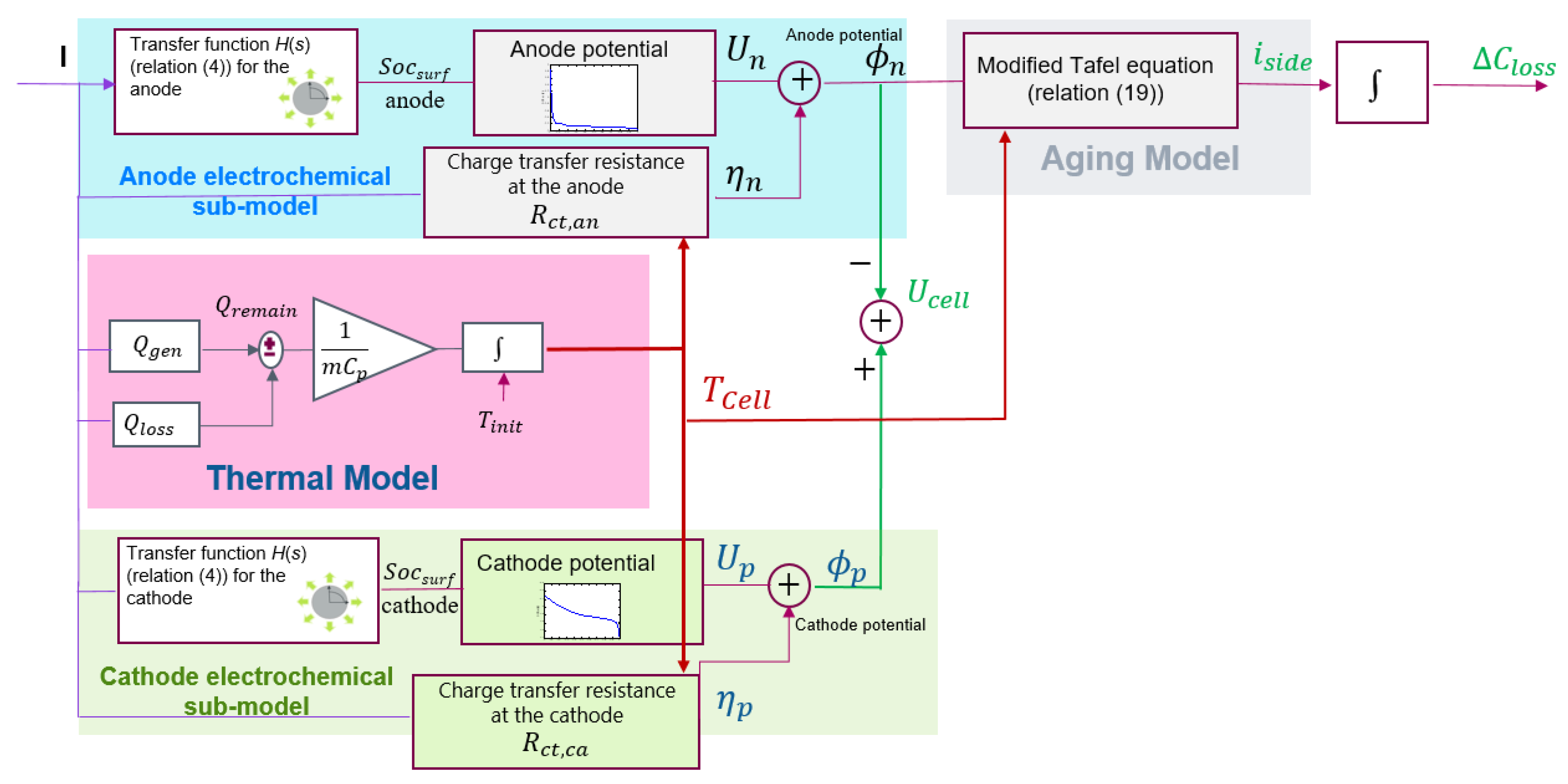
The paper is organized as follows. Section 2 describes the electro-thermal aging model that will be used in the sequel for the design of an optimal fast charging strategy. The optimal charging problem for a Li-ion battery of PHEVs (Plug-in Hybrid Electric Vehicles) is formulated in Section 3. An example of an optimal current profile and the corresponding battery model response are described in Section 4. The optimal charging problem formulated in Section 3 is solved in Section 5 with two imbricated control loops that involve robust controllers. The design of these controllers is based on a family of models that capture the nonlinear behaviour of the cell around several operating points. This family of models is computed in Section 4.2.

2. Cell Modelling

A detailed description of the lithium-ion cell model used in this work is given in [6]. It comprises three parts:

• an electrochemical part,
• a thermal part,
• an aging part.

The validation of this model and of all its parts is proposed in [6]. This paper only gives the main equations.

2.1. Description of the Electrochemical Part of the Model

The equations given in [18,19] were used to define the electrochemical part of the model. These equations result in Newman’s modelling approach [20], which leads to a pseudo 2D model and assumes that each electrode of a cell is replaced by a single spherical particle in which the Li+ ions are inserted. In the resulting particle, and through several simplifications that are given in [3], the lithium ions’ concentration gradient is described by the following diffusion equation:

$$\frac{\partial c_s}{\partial t}=\frac{D_s}{r^2}\frac{\partial }{\partial r}\left(r^2\frac{\partial c_s}{\partial r}\right)\{\begin{array}{c}{\frac{\partial c_s}{\partial t}|}_{r=0}=0\\ {D_s\frac{\partial c_s}{\partial r}|}_{r=R_s}=-\frac{j_{mean}^{Li}}{a_{s}F}\end{array}$$

(1)

In Relation (1), $J_{mean}^{Li}$ is the average of the electrode current density, r is the sphere radius and D_s is the diffusion coefficient. Resolution of the differential Equation (1) leads to the following transfer function linking the lithium concentration at the surface of the particle denoted $C_s\left(r=R_s\right)$ to $J_{mean}^{Li}$:

$$G\left(s\right)=\frac{C_s\left(r=R_s\right)}{J_{mean}^{Li}}=-\frac{R_S}{F{D}_s{a}_s\left(\sqrt{\frac{s}{D_s}}\coth \left(\sqrt{\frac{s}{D_s}}{R}_S\right)-1\right)}$$

(2)

The transfer function (2) cannot be easily simulated due to the coth function. As demonstrated in [3], it can be approximated by the transfer

$$H\left(s\right)=\frac{K_1}{s}{\left(1+\frac{s}{{\omega }_{cs}}\right)}^{0.5}$$

(3)

where the parameters $K_1$ and ${\omega }_{\mathrm{cs}}$ are functions of the coefficients of the diffusion Equation (1) (see [3]).

For a consistent initialization of the model, and also to make the variable SOC appear, the transfer function H(s) can be split into two transfer functions, such that

$$H\left(s\right)=H_{avg}\left(s\right)+H_{part}\left(s\right)$$

(4)

with

$$H_{avg}\left(s\right)=\frac{C_{s,avg}}{j_{mean}^{Li}}=\frac{K_1}{s}$$

(5)

and

$$H_{part}\left(s\right)=\frac{\mathsf{\Delta }{C}_s}{j_{mean}^{Li}}=H\left(s\right)-H_{avg}\left(s\right)=\frac{K_1}{s}\left({\left(1+\frac{s}{{\omega }_{cs}}\right)}^{0.5}-1\right)$$

(6)

In Relation (4), $H_{avg}\left(s\right)$ represents the average concentration (from the centre to the surface of the particle) and $H_{part}\left(s\right)$ is the partial gradient of ion concentration on the particle surface.

For the implementation of the battery model in a vehicle control unit, a discrete form of the transfer functions $H_{avg}\left(s\right)$ and $H_{part}\left(s\right)$ can be computed, as shown in [6]. Also, a polynomial can be used to link the lithium concentration at the surface of the particles, denoted SOC_surf, to the cell Open Circuit Potential (OCP), denoted $U_{\mathrm{n}}$ and $U_{\mathrm{p}}$ respectively for the anode and the cathode. If the charge transfer resistance is denoted R_ct (R_ct can be deduced from the Butler–Volmer equation linearization), the resulting electrochemical sub-model is represented by Figure 1.

2.2. Description of the Thermal Part of the Model

The kinetics of charge transfer during the intercalation process depends in particular on cell temperature. Cell temperature also has an impact on the kinetics of the side reactions. It is thus essential to associate a thermal model to the electrochemical sub-model. In this work, the efficient and simple thermal model presented in [21] was used to estimate the cell temperature. This thermal model results from a heat balance within the cell, and is described by

$$m{C}_p\frac{dT\left(t\right)}{dt}=Q_{gen}\left(t\right)-Q_{loss}\left(t\right)$$

(7)

The thermal parameters associated to Relation (7) are given in

Table 1. Parameters of the thermal model.

Symbol	Parameter	Unit
$m$	Mass of the cell	kg
$C_p$	Specific heat capacity	J·kg−1·K−1
$U_{pol}$	Polarization voltage	V
$R_f$	High frequency resistance	Ω
I	Input current	A
$\alpha$	Heat transfer coefficient	W·m−2·K
$A$	Cell surface area	m2
$T_{amb}$	Ambient temperature	K

. The generated heat is defined by

$$Q_{gen}\left(t\right)=U_{pol}\left(t\right)I\left(t\right)+R_{f}I{\left(t\right)}^2$$

(8)

In Relation (8), U_pol(t) is the irreversible heat generation due to electrode polarization. $R_{f}I{\left(t\right)}^2$ models heat losses over the internal resistor of $R_f$.

The convective heat exchanged with the environment is:

$$Q_{loss}\left(t\right)=\alpha A\left(T\left(t\right)-T_{amb}\right)$$

(9)

2.3. Description of the Aging Part of the Model

Depending on the intended application, fast charging or battery cycling until End of Life (EOL), a short-term or a long-term model is required. In this work, the developed model is devoted to designing fast charging algorithms, and aging is considered to be mainly caused by the growth of a Solid Electrolyte Interphase (SEI) layer on the anode. This degradation mostly happens during short to middle-term battery usage during fast charging cycles. The aging model used is based on the equations proposed in [22] and, following the observations from post-mortem analysis of the investigated cells, aging is only considered on the anode electrode. For a constant temperature T, the current produced by the side reaction leading to the undesired reduction of Li ions is defined by the Tafel equation

$$j_{sr}=-a_s^n{j}_{0,sei}exp\left(-\frac{nF{\alpha }_n}{RT}{\eta }_{sei}\right)$$

(10)

If ${\phi }_{en}$, $R_{sei}$ and $U_{sei}^{ref}$ denote respectively the anode potential, the inner resistance of the SEI layer and the reference potential of SEI formation (assumed to be 0.4 V), the SEI overpotential is given by the relation

$${\eta }_{sei}={\phi }_{en}-R_{sei}I-U_{sei}^{ref}$$

(11)

in which the anode potential ${\phi }_{en}$ is defined by

$${\phi }_{en}={\eta }_n+U_n+R_{sei}I$$

(12)

According to [23], ${\eta }_n$ is deduced from the Butler–Volmer equation which defines the kinetics of Li ion intercalation, and can be approximated by

$${\eta }_n=\frac{2RT}{F}\log (\left(\frac{j_I}{2a_s^n{j}_0^n}\right)+\sqrt{{\left(\frac{j_I}{2a_s^n{j}_0^n}\right)}^2+1})$$

(13)

for an easier implementation. The electrochemical parameters associated with Relations (10) to (13) are defined in

Table 2. Aging sub-model parameters.

Symbol	Parameter	Unit
$a_s^n$	Specific surface area	m−1
$j_{0,sei}$	Exchange current density	A·m−2
${\alpha }_n$	Symmetry factor	-
n	Number of transferred electrons	-
$E_a$	Activation Energy	kJ·mol−1
${\delta }_{sei}$	SEI layer thickness	m
$M_{sei}$	Molar mass of SEI layer	kg·mol−1
$\rho$	Density of SEI layer	kg·m−3
${\kappa }_{sei}$	SEI layer conductivity	S·m−1
$R_{sei,init}$	Initial resistance of SEI layer	Ω·m2
$R_p$	Resistance of side reaction product	Ω·m2
$I_{ch}$	Charging current	A

. Some parameters are taken from [22]. The others were estimated using measurements on the cell under investigation.

The increase in temperature resulting from fast charging operation has a large impact on the side reaction rate. Thus, Relation (10) must be modified to take into account the Arrhenius dependency of the side reaction current on the temperature variation. The modified Equation (10) is thus given by

$$j_{sr}=-a_s^n{j}_{0,sei}exp\left(\frac{E_a}{R}\left(\frac{1}{T_{ref}}-\frac{1}{T}\right)\right)exp\left(-\frac{nF{\alpha }_n}{RT}{\eta }_{sei}\right)$$

(14)

The SEI thickness (δ_sei) and resistance (R_sei) can be computed by the following Relations [22]:

$$\frac{\partial {\delta }_{sei}}{\partial t}=\frac{M_{sei}}{2F\rho }{j}_{sr}$$

(15)

$$R_p\left(t\right)=\frac{{\delta }_{sei}{}_{}}{{\kappa }_{sei }}$$

(16)

$$R_{sei}\left(t\right)=R_{sei,init}+R_p\left(t\right)$$

(17)

Experimental observations [24] have shown that, after a primary formation and after some cycles, the SEI layer thickness growth at the surface of the electrode decreases. To model such a behavior, an exponential function was associated to Relation (18), which becomes

$$j_{sr}=-a_s^n{j}_{0,sei}exp\left(-\lambda {\delta }_{sei}\right)exp\left(\frac{E_a}{R}\left(\frac{1}{T_{ref}}-\frac{1}{T}\right)\right)exp\left(-\frac{nF{\alpha }_n}{RT}{\eta }_{sei}\right)$$

(18)

where $\lambda$ is the SEI decay rate constant (m⁻¹). To obtain this coefficient, it is assumed that, after some cycles, the SEI thickness stabilizes.

To guarantee an efficient fast charging strategy, the aging sub-model must also reproduce with good accuracy the higher capacity loss that has been observed at higher charging C-rates. This requirement is not permitted with Relation (18). Thus, to scale the inverse Butler-Volmer overpotential η_n, a coefficient K_η is introduced in Equation (18), which thus becomes

$$j_{sr}=-a_s^n{j}_{0,sei}exp\left(-\lambda {\delta }_{sei}\right)exp\left(\frac{E_a}{R}\left(\frac{1}{T_{ref}}-\frac{1}{T}\right)\right)exp\left(\frac{-nF{\alpha }_n}{RT}\left(K_{\eta }{\eta }_n+U_n-U_{sei}^{ref}\right)\right)$$

(19)

with $C_T=-a_s^n{j}_{0,sei}exp\left(\frac{nF{\alpha }_n}{RT}{U}_{sei}^{ref}\right)exp\left(\frac{E_a}{R{T}_{ref}}\right).$

In Relation (19), it can be noticed that the time-dependent (calendar) aging effects and current-dependent (cycling) aging effects are decoupled. This offers the possibility of better interpreting the influence of each mechanism on cell aging, and of emphasizing the influence of the C-rate on the decrease in capacity during cycling and in particular rapid charges.

To the best knowledge of the authors, the physics-based battery model proposed in this study, which takes into account degradation mechanisms as a function of SOC, temperature and C rate, is unprecedented in the literature. These characteristics also allow a very good correspondence between the response of the model and the measurements.

2.4. Whole Cell Model

The electro-thermal aging model described in the previous paragraphs can be represented by the block diagram of Figure 1. In this figure, the sub-models denoted ‘Anode’ and ‘Cathode’ are deduced from the description performed in Section 2.1. The thermal model of Section 2.2 provides the cell temperature information from the current applied to the aging model described in Section 2.3. This model has been validated by several tests, as described in [6].

Regarding the tuning of the parameters associated with this model, it can be partially accomplished using information provided by the battery manufacturer. Tests are required to tune the remaining parameters. The tuning methodology is described in [5], and needs to be applied for each new type of battery. As no feedback exists between the aging model and the electrochemical sub-models, the model can fit the behaviour of the battery only within a given aging range (this is enough to get the battery state estimation during a charge). The Model of Figure 1 must be adjusted (on board) periodically to take into account the impact of aging on some parameters of these sub-models (OCP functions, charge transfer resistance, …).

Further studies can be conducted (see [3]) to include the electrolyte dynamics in the anode and cathode electrochemical sub-models. Considering the ion diffusion phenomenon inside the electrolyte would increase the model accuracy in estimation of the terminal voltage, but would also increase the model’s complexity.

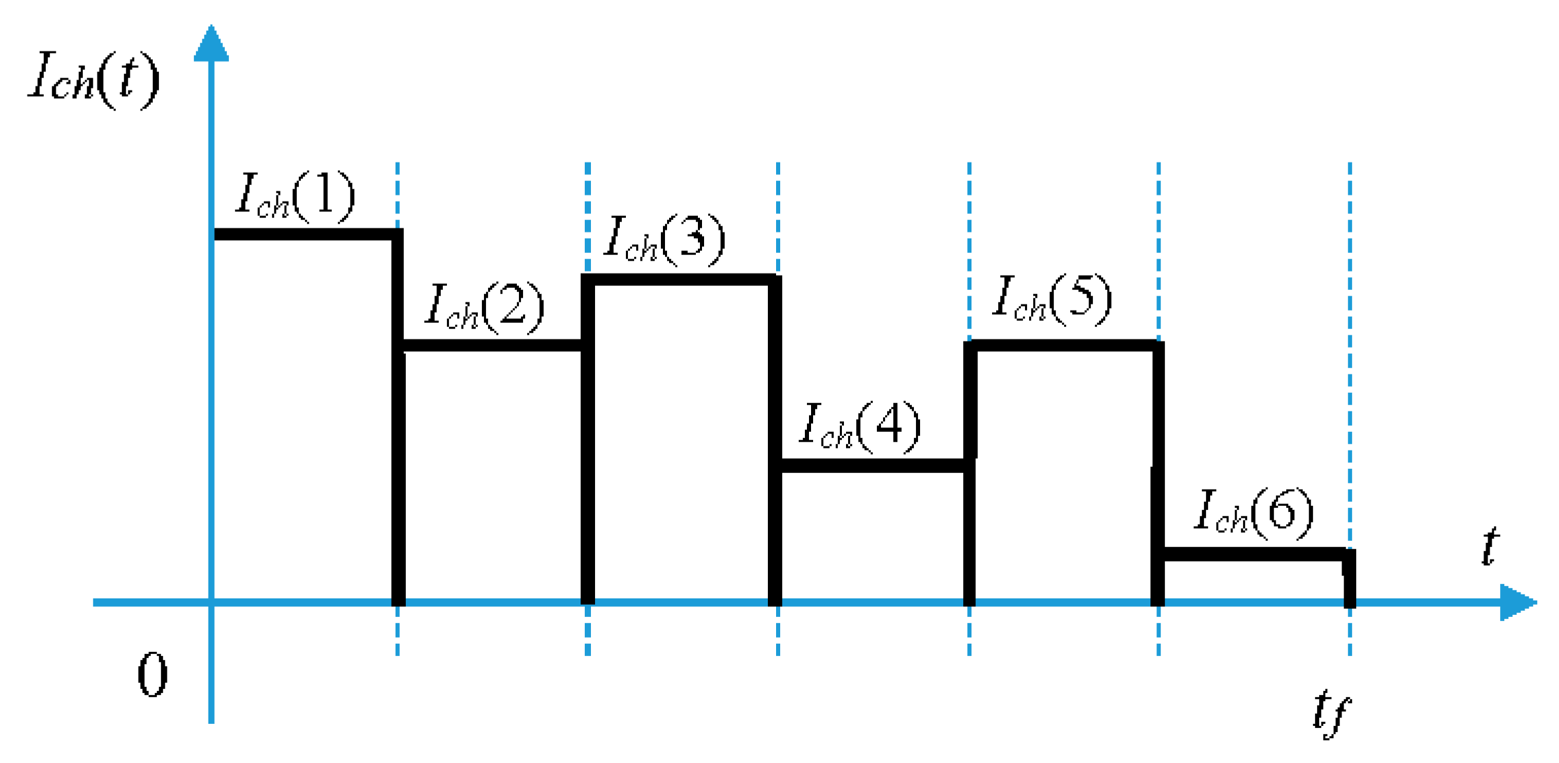
3. Trajectory Planning

The fast charging strategy developed in this paper, which can be integrated in a battery management system (BMS), is described globally by Figure 2. In this diagram, the model presented in Section 2 is used in the battery observer to simulate the battery behavior under various operating conditions. Using measures of the cell current $I_{Charge}$, voltage $U_{cell}$ and temperature $T_{cell}$, this observer estimates (among other information) the cell capacity fade $\Delta C_{fade}$. This information is used by a fast charging controller that adapts the charge current magnitude to follow a charge profile $I_{ref}$ while reducing the cell capacity fade during recharge.

The function of the charging controller is to determine the optimal charging current profile imposed on the battery. The optimal current is that which minimizes the recharging time (therefore the highest possible) while limiting a variable upper limit on the current. This makes it possible to meet a rapid recharging target without increasing battery aging too much. The strategy adopted in this work to determine the optimal charging profile thus consists in computing offline the side reaction current before battery charging. The side reaction current changes over time and is a function of the SOC and of the charging current. If the charging process is split into a finite number of time slots, a lookup table can provide the limit on the side reaction current on each interval as a function of SOC. The side reaction current limit provided on each slot defines the side reaction current trajectory. The controller thus computes the corresponding charging current and defines in real time the optimal profile of the charging current to meet the calculated side reaction current trajectory.

In practice, to acheive the optimal charging trajectory, the capacity loss during a fixed charging time t_f of twenty minutes is minimised under the following constraints:

• bounds on the charging current (Ich), in order to avoid exceeding the maximum charge current limits (3.5 C) for safety reasons,
• an increase in the SOC from 5% to 80% (but other ranges of SOC variation can be defined).

Denoted in the sequel is a Multi-stage Constant Current (MCC) of duration $t_f$, a charge current profile made of a series of N pulses (or slots) of the same duration ($t_f/N$), in which each pulse can have a different magnitude (thus N degree of freedom in the current profile that can be optimised). An example of an MCC profile is represented in Figure 3. It is used for its flexibility in the definition of a profile in order to maximize energy efficiency and to improve battery life during fast charging [25]. The optimal control problem can thus be analytically defined by

$${\displaystyle \underset{I_{ch}\left(t\right)}{\min }}{{\displaystyle \int }}_0^{t_f}\mathsf{\Delta }{C}_{loss}\left(t\right)dt$$

(20)

subject to

$$\dot{x}\left(t\right)=f\left(x\left(t\right),I_{ch}\left(t\right)\right),x\left(0\right)=x_0$$

(21)

$$\frac{1}{3600}{{\displaystyle \int }}_0^{t_f}{I}_{ch}\left(t\right)dt\ge Q_{trans}$$

(22)

$$0\le I_{ch}\left(t\right)\le 3.5C$$

(23)

in which Q_trans denotes the Li-ion charges stored in (Ah), ΔC_loss denotes the capacity loss (Ah), and t_f (s) is the charging time. Sequential Quadratic Programming (SQP) is used to solve the optimal control problem defined by Relations (20) to (23) for various operating conditions.

Variations of SOC, anode potential, side reaction and capacity loss variation at 35 °C obtained after optimisation with only 4 slots are shown in Figure 4. These curves are compared to those obtained with a conventional Constant Current Constant Voltage (CCCV) profile. This kind of charge profile has been chosen for comparison purposes because it is very commonly used for recharging batteries (lithium ion or not). This figure shows a decrease in capacity loss close to 15% with the optimal current profile in comparison with the CCCV profile. The optimisation was performed for various aging levels, various ambient temperatures (10, 17, 27, 30, 47, and 77 °C) and for various states of health from End of Life (EOL), Middle of Life (MOL) and Beginning of Life (BOL).

These results were obtained with a cell whose dynamical behaviour is assumed to be perfectly known. This is an ideal case that does not exist in practice due to modelling uncertainties, and applying the optimal charging current profiles obtained does not necessarily minimize aging while reaching the target SOC. To take into account the modelling uncertainties, a closed loop strategy must be implemented. As shown in the next section, the side reaction current J_sr that creates aging was defined as the control signal to control the battery charging due to its high sensitivity to the charging current, as illustrated by Figure 4.

4. Cell Model Linearization

The interest of closed-loop control for fast charging has been highlighted in Section 1 and Section 3. The design of a linear controller to implement such a loop is thus the objective of this section. The block diagram of the cell model in Figure 1 suggests that the cell is highly nonlinear. This is confirmed by the simulations of this model, which show a high sensitivity to temperature, lifetime stage and charging current level. Such a nonlinear behaviour is taken into account in the approach presented here with a linearized model set that is computed for a set of operating points (temperature, charging current, stage of life) and various optimal charging profiles, and thus side reaction current (J_sr) profiles.

4.1. State-Space Model of the Cell Model

The following nonlinear state-space model:

$$\{\begin{array}{c}\dot{x}\left(t\right)=f\left(x\left(t\right), u\left(t\right)\right)\\ y\left(t\right)=g\left(x\left(t\right), u\left(t\right)\right)\end{array}$$

(24)

represents the battery model in which the input u(t) is the charging current I_ch(t). The state vector x(t) and the output vector y(t) are respectively given by

$$y={\left[J_{sr},U_{bat},{\varphi }_{en},OCV,T,SOC\right]}^T$$

(25)

$$x={\left[\mathsf{\Delta }{C}_{loss},{\delta }_{SEI},C_{avg,n},C_1^{part,n}\dots C_5^{part,n},C_{avg,p},C_1^{part,p}\dots C_5^{part,p}\right]}^T$$

(26)

where the variables that appear in Relations (25) and (26) are defined in

Table 3. Variables in the state and output vectors of the nonlinear cell model * I = p (cathode), n (anode).

Symbol	Parameter	Unit
$\mathsf{\Delta }{C}_{loss}$	Capacity loss	mAh
${\delta }_{SEI}$	Thickness of SEI layer	m
$C_{avg,i^{ *}}$	Electrode average concentration	Ah
$C_1^{part,i{}^{*}}$	Electrode partial concentration	Ah
$U_{bat}$	Battery terminal voltage	V
${\varphi }_{en}$	Anode potential	V
$OCV$	Open Circuit Voltage	V

.

The next section describes the approach used to derive a set of linear models (one model for a given operating point) for the approximation of the nonlinear cell model.

4.2. Operating Points Definition

The optimal charging profiles computed in Section 3 were used to define the operating points required for the linearization of the nonlinear model (24). The optimization was performed for various aging levels and ambient temperatures, with SOC within 5–80%. For all optimal current profiles, relaxation intervals were added to reach equilibrium conditions during the constant current phases of the MCC profile. 432 operating points were finally considered, made up of 18 ambient (and internal) temperatures, three aging levels and eight operating conditions for each charging profile.

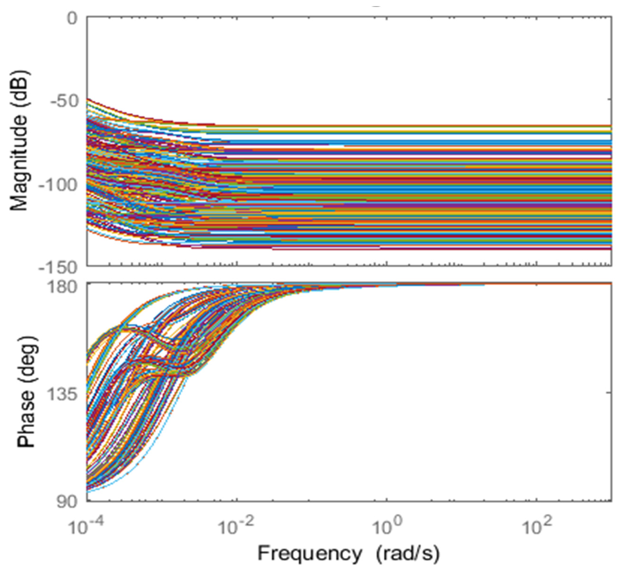
4.3. Uncertain Linear Models Resulting from the Nonlinear Battery Model

The nonlinear model (24) was linearized around operating points using a numerical method (Matlab linmod command). The Bode diagrams of the resulting set of linear models of the transfer function J_sr(s)/I_ch(s) are shown in Figure 5. Among this set, one was chosen as a nominal model, with the other linear model thus defining an uncertain linear model. Figure 5 highlights a strong dependence of the frequency response of the transfer function J_sr(s)/I_ch(s) to the operating point. The resulting gain and phase uncertainty are taken into account in the next section for the design of a fast charging robust controller.

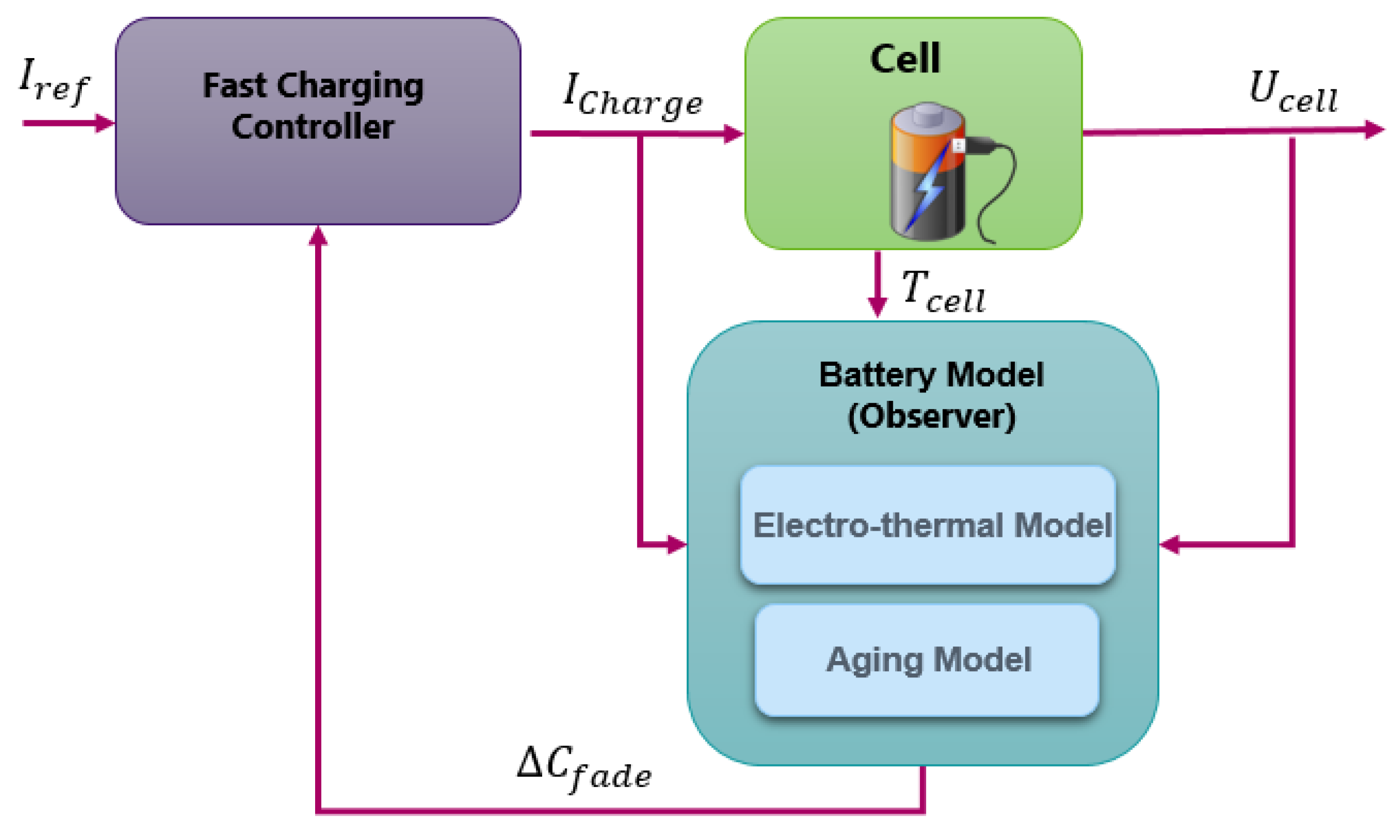
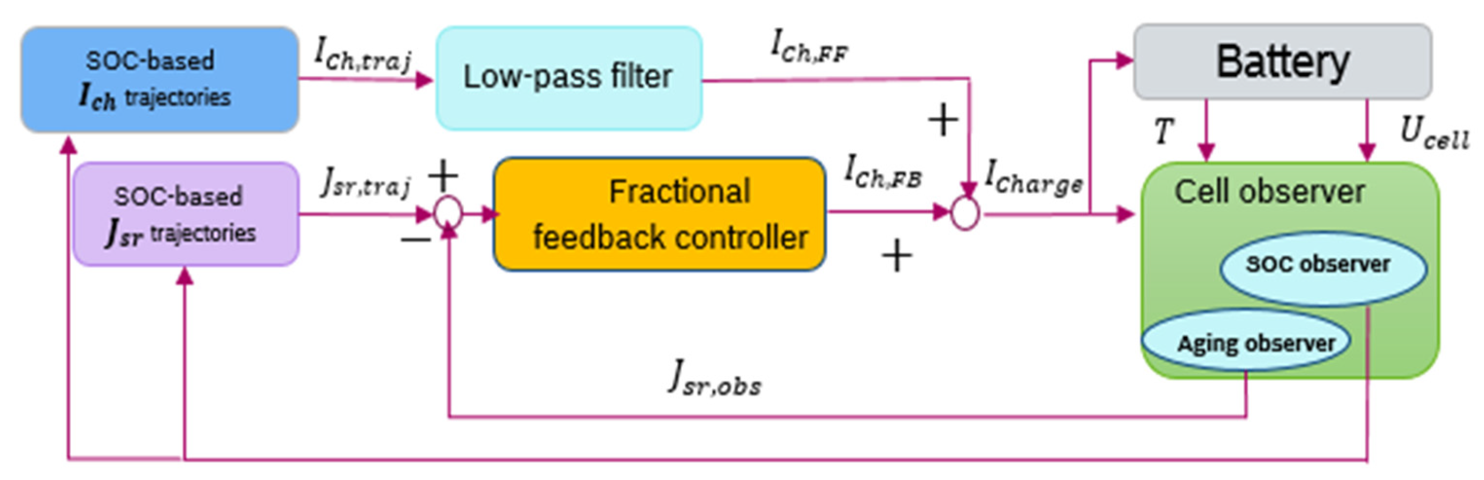
5. Design of the Fast Charging Robust Controller

5.1. Closed-Loop Control

The objective was to design a two-degrees of freedom fast charging controller, as illustrated by Figure 5. In such a control scheme, the feedforward must ensure the initialization of the plant input, and the robust feedback must permit the desired accurate output tracking. The plant model output J_sr,traj and input I_Ch,traj reference signals (optimal trajectories) are known and provided by the optimal MCC trajectory planning.

As shown in Figure 6, a low pass filter was implemented for the reference current profile smoothing. With the control scheme of Figure 6, if the battery behaviour fits the one used for the charging profile optimisation, the charging current I_Charge that makes it possible to track the optimal J_sr,traj is equal to the feedforward current I_Ch,FF. The feedback controller thus has no effect. Conversely, if the battery behaviour differs from the behaviour of the model used for the optimisation of the charging profiles, the feedback loop adapts the charging current. It imposes the computed optimal side reaction current on the cell. As only cell temperature T, charging current I_Charge and voltage U_cell, are measureable signals, an aging observer using the cell model was designed to estimate the side reaction current.

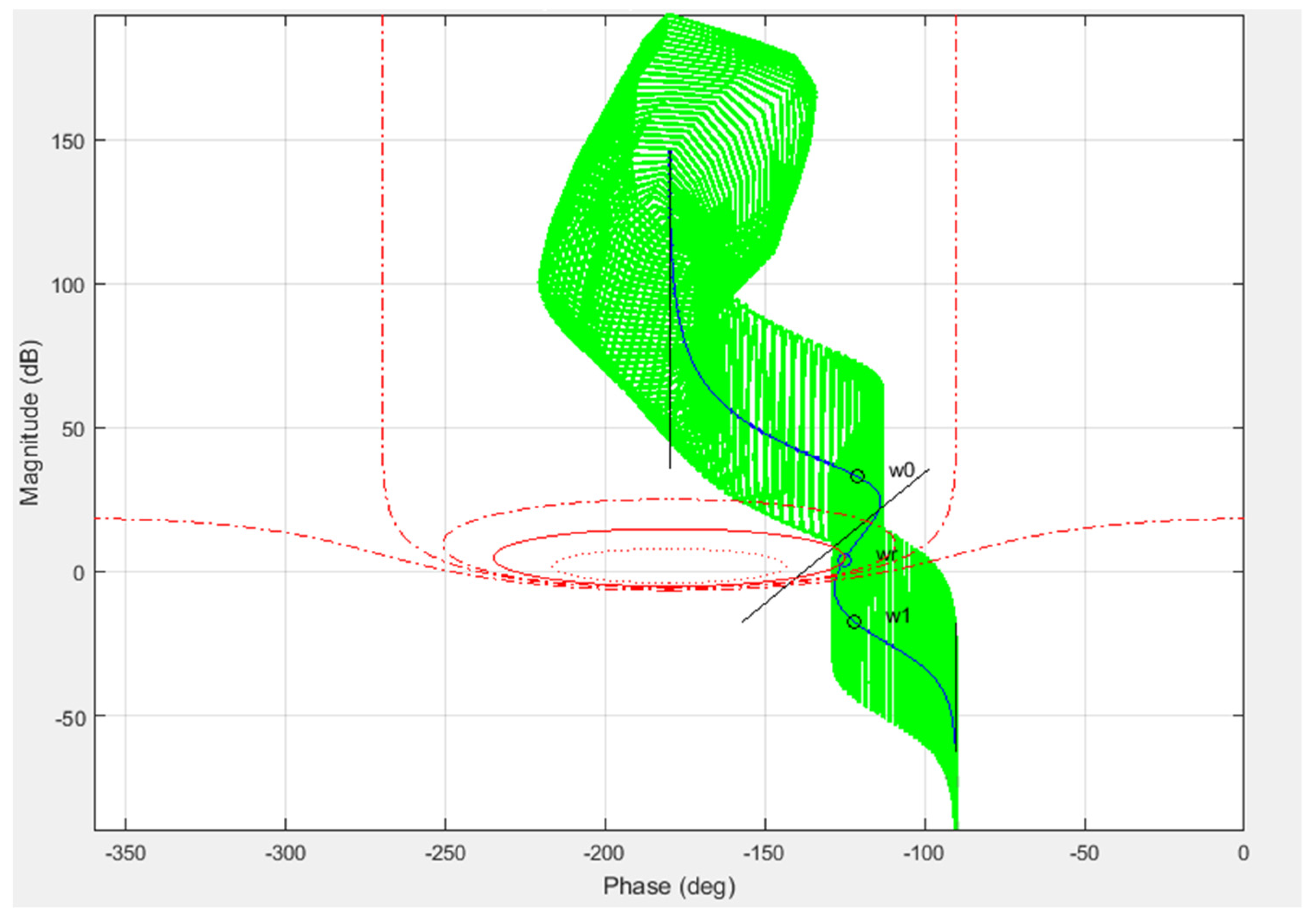
5.2. CRONE Control Methodology for Robust Controller Design

The controller C(s) in Figure 6 was designed using the CRONE control methodology. It uses fractional differentiation to define high-level design parameters [26] that are tuned in the frequency domain. The third generation CRONE control was used in this work. It is based on the optimization of the transfer function β_nom(s) parameters (β_nom(s) being computed for the nominal plant denoted G_nom) defined by

$${\beta }_{nom}\left(s\right)={\beta }_l\left(s\right){\beta }_m\left(s\right){\beta }_h\left(s\right)$$

(27)

in which β_l(s) is an integer proportional integrator of order n_l defined by

$${\beta }_l\left(s\right)=C_l{\left(\frac{{\omega }_{N^{-}}}{s}+1\right)}^{n_l}$$

(28)

β_m(s) groups several band-limited generalized templates

$${\beta }_m\left(s\right)={\displaystyle \prod }_{k=-N^{-}}^{N^{+}}{\beta }_{mk}\left(s\right)$$

(29)

with

$${\beta }_{mk}\left(s\right)=C_k{\left({\alpha }_k\frac{1+\frac{s}{{\omega }_{k+1}}}{1+\frac{s}{{\omega }_k}}\right)}^{a_k}{\left({\Re }_i\left\{{\left({\alpha }_k\frac{1+\frac{s}{{\omega }_{k+1}}}{1+\frac{s}{{\omega }_k}}\right)}^{i{b}_k}\right\}\right)}^{-q_{k}sign\left(b_k\right)}$$

(30)

where ${\alpha }_k={\left(\frac{{\omega }_{k+1}}{{\omega }_k}\right)}^{0.5}$ for $k\ne 0,$ and ${\alpha }_0={\left(\frac{1+{\left(\frac{{\omega }_r}{{\omega }_0}\right)}^2}{1+{\left(\frac{{\omega }_r}{{\omega }_1}\right)}^2}\right)}^{0.5}$ and β_h(s) is a low-pass filter of order n_h:

$${\beta }_h\left(s\right)=C_h{\left(\frac{s}{{\omega }_{N^{+}}}+1\right)}^{-n_h}$$

(31)

Order $n_l$ must be adjusted to get the desired controller accuracy. The constants $C_l$, $C_k$ and $C_h$ are tuned to ensure a given resonance frequency ${\omega }_r$ of the closed loop transfer function T_nom(s) = β_nom(s)/(1 + β_nom(s)). Order $n_h$ was chosen to ensure a bi-proper or strictly proper controller. The open-loop parameters are tuned M_T, where M_T denotes the resonance peak of the complementary sensitivity function T(s). Such an objective is attained by minimizing the objective function

$$J={\displaystyle \underset{G}{sup}}{M}_T-M_{Tnom}$$

(32)

in which M_Tnom denotes a whised value for the closed-loop resonance peak computed with the nominal plant denoted G_nom. The minimisation of Relation (32) is achieved under the constraints on the four closed loop sensitivity functions that follows:

$$\begin{gathered} {\displaystyle \underset{G}{inf}}\left|T\left(j\omega \right)\right|\ge T_l\left(\omega \right),{\displaystyle \underset{G}{sup}}\left|T\left(j\omega \right)\right|\le T_u\left(\omega \right) \\ {\displaystyle \underset{G}{sup}}\left|S\left(j\omega \right)\right|\le S_u\left(\omega \right),{\displaystyle \underset{G}{sup}}\left|CS\left(j\omega \right)\right|\le C{S}_u\left(\omega \right) \\ {\displaystyle \underset{G}{sup}}\left|GS\left(j\omega \right)\right|\le G{S}_u\left(\omega \right) \end{gathered}$$

(33)

with

$$\{\begin{array}{c}T\left(s\right)=\frac{G\left(s\right)C\left(s\right)}{1+G\left(s\right)C\left(s\right)} S\left(s\right)=\frac{1}{1+G\left(s\right)C\left(s\right)} \\ CS\left(s\right)=\frac{C\left(s\right)}{1+G\left(s\right)C\left(s\right)} SG\left(s\right)=\frac{G\left(s\right)}{1+G\left(s\right)C\left(s\right)}\end{array}$$

(34)

Using the Nichols plot, by minimizing criterion J in Relation (32), the optimal parameters move the frequency uncertainty domains so that they cover areas of low stability margin as little as possible around the (−180, 0 dB) critical point on the Nichols chart (as the open-loop frequency response uncertainty domains are those of the plant). Only a nonlinear optimization method can be used to compute the optimal parameters as uncertainties are not norm-bounded and taken into account by the least conservative method. If N⁺ = N⁻ = 0 in Relation (29), only the independent four parameters ω₀, ω₁, ω_r and Y_r=|β(jω_r)|_dB need to be optimized in Relation (27). In the Nichols chart, the tangency of the frequency response β_nom(jω) to the desired M_Tnom circle can be ensured by computing the other parameters of Relation (27), such as a₀ and b₀. The optimal open loop transfer function being found, the controller C(s) can be obtained with the ratio of the optimal open-loop frequency responses by the nominal plant defined by

$$C_F\left(j\omega \right)=\frac{{\beta }_{nom}\left(j\omega \right)}{G_{nom}\left(j\omega \right)}$$

(35)

From this frequency response, a frequency domain system identification method can be used to obtain the coefficients of an integer transfer function C(s) whose frequency response fits the frequency response of C_F(s). Such a method has the real advantage of producing a controller whose order is rather low (classically less than 6) whatever the problem.

To conclude, as the over-estimation of plant perturbation is avoided, the CRONE control methodology permits a non-conservative robust control system, and thus, in the majority of applications, better performance.

5.3. Design of a CRONE Controller for Fast Charging

The frequency responses of the linear models obtained through the linearization of model (24) (see Section 4.2) for various operating conditions (temperature, aging, SOC) are shown on Figure 5. This figure highlights that, in low and high frequencies respectively, the gains of the linear models are of order 1 and 0. Thus, for a low-pass filter behaviour of the controller in high-frequencies and as an integrator in low-frequencies, the open-loop orders $n_l$ and $n_h$ are defined such that $n_l=2$ and $n_h=1$. The minimization of the complementary sensitivity function resonance peak variation according to Relation (32) is acheived under the design specifications that follows:

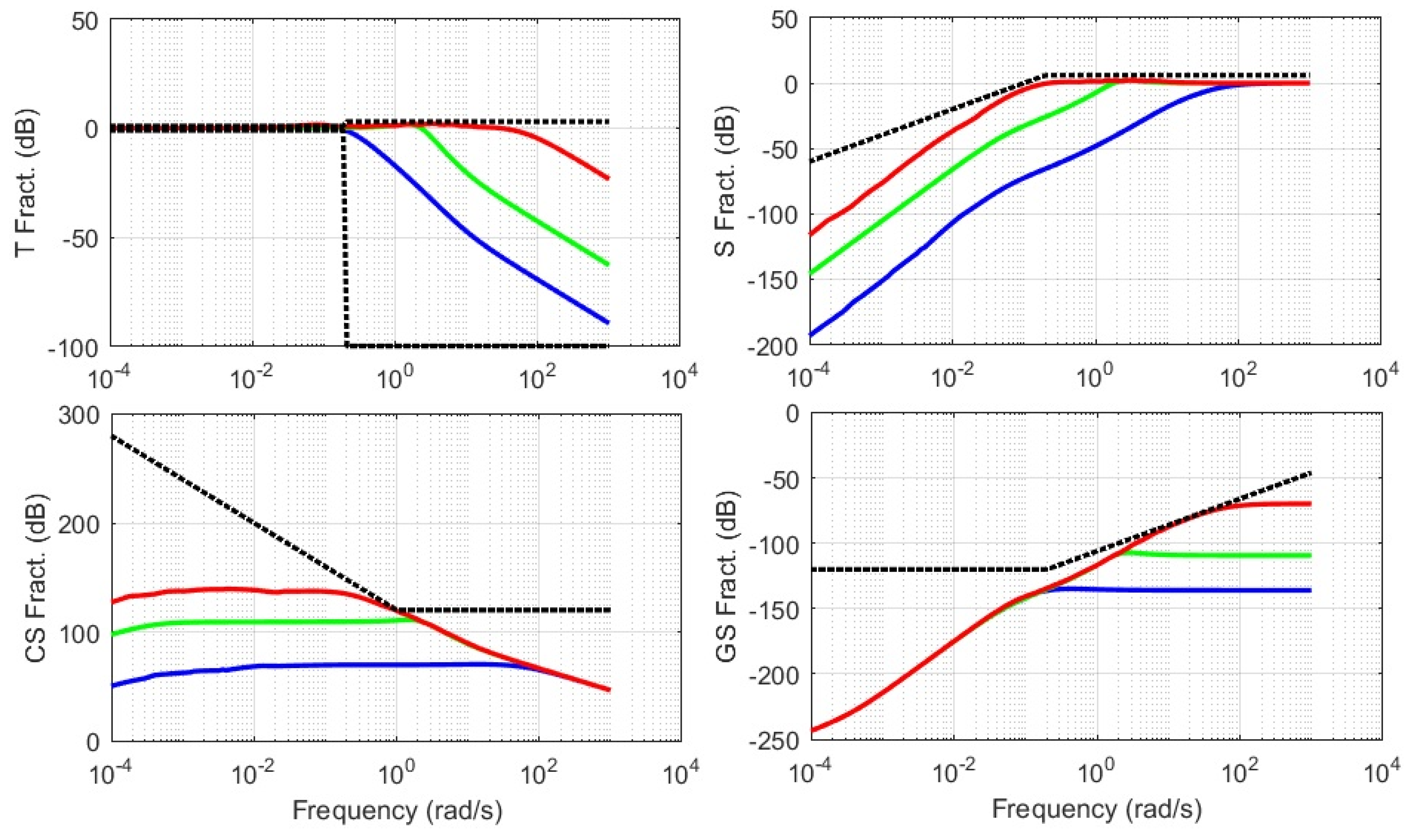
• a sensitivity function S(s) resonance peak lower than 6dB to reach a good stability degree;
• a nominal resonance peak $M_{Tnom}$ of function T(s) equal to 1.7 dB for a small overshoot of the nominal response to a step of the reference signal of $J_{sr}$;
• a closed loop bandwidth close to 0.2 rad/s;
• a control effort sensitivity less than 10 A ($I_{ch}$) for a variation of $J_{sr}$ of 10 μA in high-frequency.

The CRONE control toolbox [27,28] was used to compute the open-loop transfer function optimal parameters that meet the above specifications. The optimal parameters obtained are the following: $Y_r=3.8\mathrm{dB}$, ${\omega }_r=1.5\mathrm{rad}·{\mathrm{s}}^{-1}$, ${\omega }_0=0.1\mathrm{rad}·{\mathrm{s}}^{-1}$ and ${\omega }_1=7.5\mathrm{rad}·{\mathrm{s}}^{-1}$, leading to the following values for the fractional integration orders: $a_0=1.42$ and $b_0=-0.46$. The resulting open loop transfer function Nichols chart for the nominal behaviour and the associated uncertainty domains is shown in Figure 7. The values of ${\omega }_{\mathrm{r}}$, ${\omega }_0$ and ${\omega }_1$ appear on this figure. This figure demonstrates that the closed-loop system is stable, as all the behaviours are far from the instability point (−180°, 0 dB) area. Figure 8 shows the gain diagram of the four sensitivity functions T(s), S(s), GS(s) and CS(s) for the nominal behaviour of the plant and for two extreme behaviours of the plant. The user defined constraints (dotted lines) are also represented. As the gain of all the sensitivity functions does not exceed the constraints defined, it can be concluded that the design specifications are met. The closed loop robustness is also demonstrated by the small resonance peaks of the functions S(s) andT(s). An order 4 rational controller C(s) is finally obtained using the method described at the end of Section 5.2. As the controller obtained contains an integrator, an anti-windup configuration is included in the control system. It cancels the charge current increase due to the output integrator saturation, thus meeting the current limits for the considered battery (a safety charge current limit of 3.5 C).

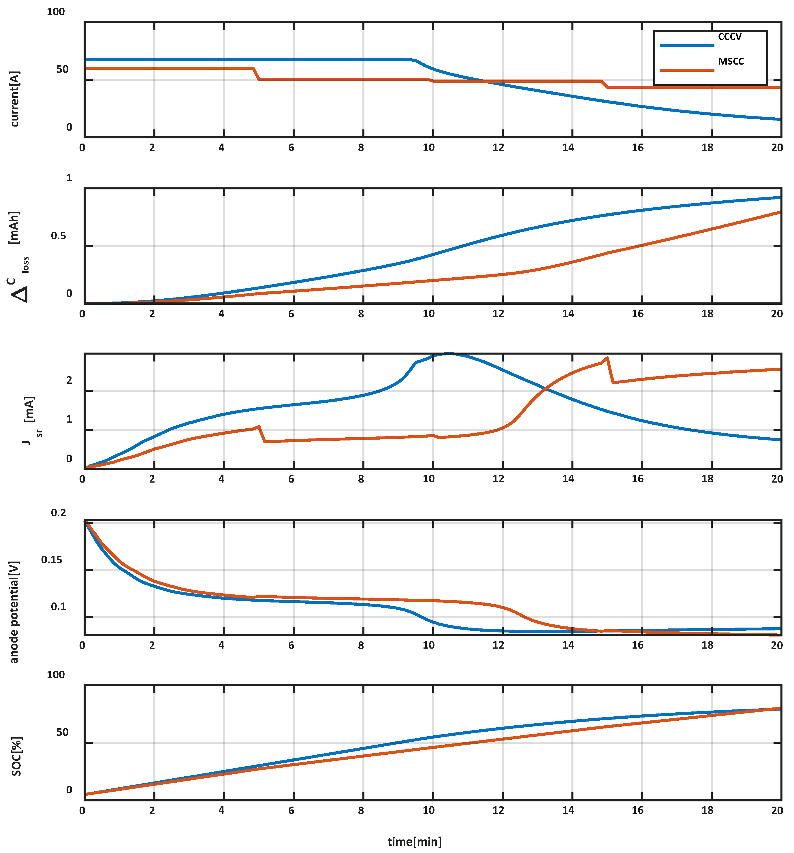
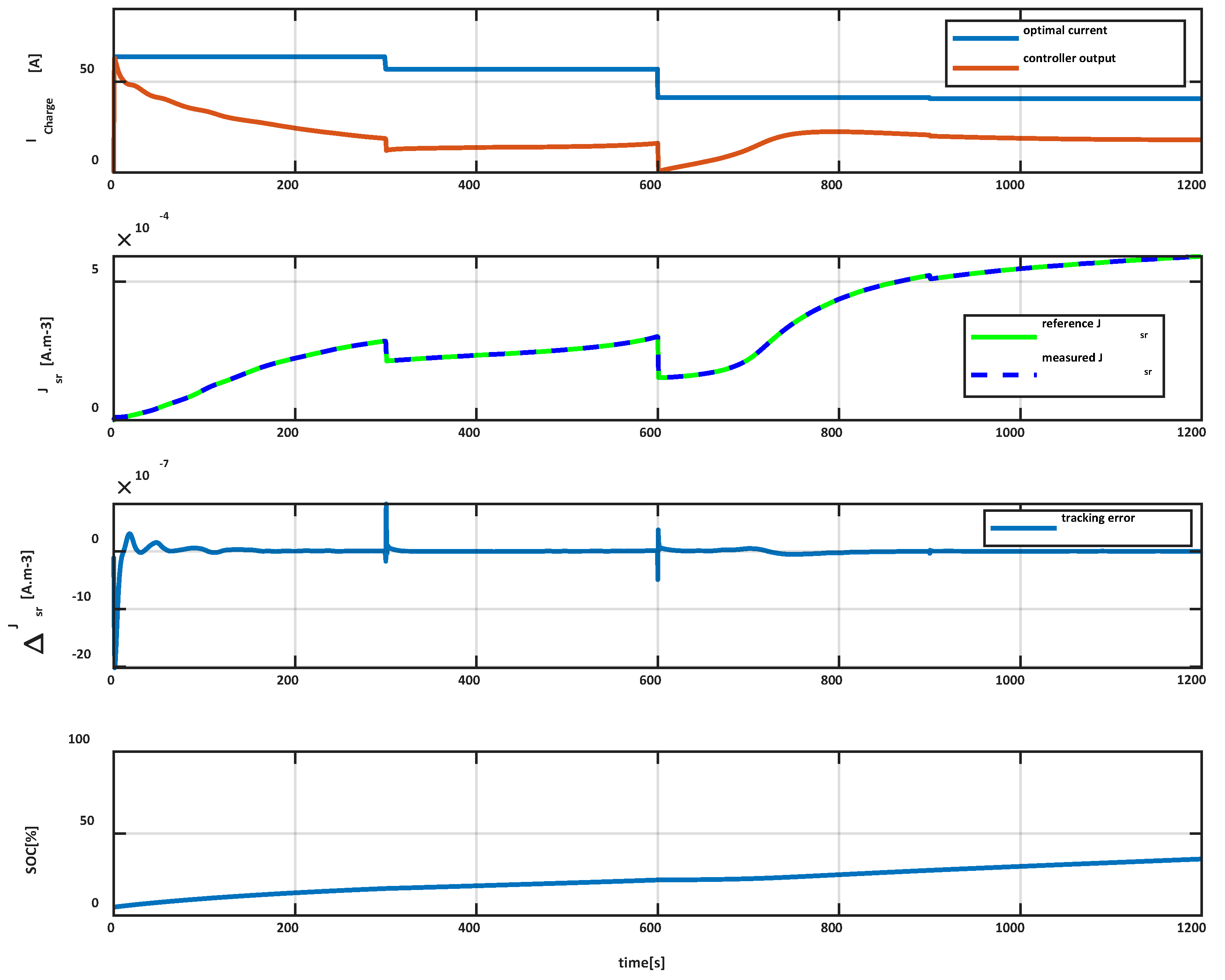
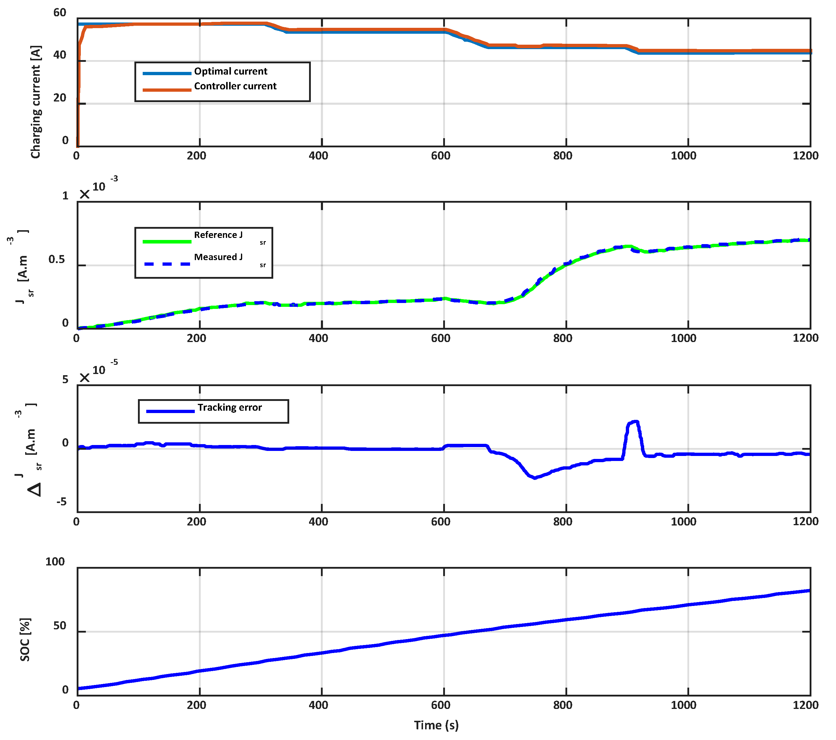
5.4. Analysis of the Control Loop Performance

The fast charging controller previously designed was applied to the model (nonlinear) of the battery described in Section 2.3. As previously mentioned, this model has a large sensitivity to aging and temperature, and the closed loop system sensitivity and robustness to these parameters must be verified. It is achieved by studying the impacts of battery parameters variations on the closed loop system response. As an example, Figure 9 shows the optimized side reaction profile tracking (profile computed as in Section 3) for the cell at BOL and for a temperature of 10 °C. The simulation is performed with a model whose parameters defining the cell aging, the initial SEI layer thickness (nm), the cell high frequency resistance (Ω), the cell capacity (Ah) and the specific surface area of the anode (${\mathrm{m}}^{-1}$) were changed by $~\pm 20\%$. The J_sr diagram in the figure shows a tracking error close to 2 (μA·m⁻³). In spite of plant uncertainties, the controller tracking performance is thus guaranteed.

5.5. Improvement of the Control Strategy

As it cannot be guaranteed that the final value of the SOC will be reached with the strategy previously defined, some modifications must be made, and are now proposed to correct the situation. As shown in Figure 10, the control scheme of Figure 5 is completed by a loop that rescales the charging current I_Charge and side reaction current J_sr,_traj optimal trajectories against SOC.

Variations in some parameters of the battery model, such as electrolyte resistance, initial temperature and initial SEI layer, were carried out to evaluate the robustness of the modified charging strategy. The simulations performed with a cell at its BOL, and for an ambient temperature of 10 °C, are shown in Figure 11. This figure proposes a comparison between the current produced by the controller and the optimal charging current defined by the trajectory planning strategy. It highlights that the controller output moves away from the optimal current profile to maintain the optimal side reaction current tracking represented on the second diagram of Figure 10. As shown by the third diagram of Figure 11, this leads to a negligible tracking error. Using the control scheme of Figure 10, Figure 11 shows that, within the desired charging time of 20 min, the target SOC of 80% is reached.

In spite of its efficiency, the control loop of Figure 10 cannot be implemented easily in a car controller. The charging controller indeed requires the computation of the side reaction current and charge current trajectories. They are obtained after the optimization of a charging profile using the method described in Section 3. However, this optimization problem involves a large number of parameters and requires the implementation of a nonlinear optimization routine. Such an approach is highly time and resource consuming, and prevents any implementation in a car BMS. This is why the authors have also designed an efficient profile optimization method, which is patent pending.

6. Conclusions

A solution for lithium-ion battery optimal fast charging was proposed in this paper. Optimality here relates to battery aging minimization, which is achieved by tracking specific charging and side reaction current reference trajectories (optimal trajectories) using a feedforward–feedback control loop. The optimal trajectories are computed using an algorithm involving an electro-thermal battery aging model recalled in this paper and developed in [6] by the same authors. This electro-thermal battery aging model also permits the display of dynamic behaviors quite different from a lithium-ion cell in relation to age and temperature. This sensitivity problem is taken into account in the charging strategy proposed using a robust CRONE feedback controller. The performance of the closed loop approach proposed is highlighted by improved side reaction current trajectories tracking, thus leading to reduced aging during fast charging. To the best knowledge of the authors, this is the first time that a closed-loop strategy, coupled with an electro-thermal battery aging model for fast charging while taking into account battery health, has been proposed in the literature.

Most of the proposed algorithms and methods in this thesis were validated by means of simulations. The evaluation of the internal battery states is not possible using real cells and measurements, but simulation provides this possibility. However, the importance of experimental validations cannot be ignored, and thus should be pursued in a future work. Upon the successful validation of the simulation results presented in this work, the electro-thermal aging battery model and the intelligent charging strategy can be implemented as a part of a BMS.

References

1. Botte, G.; Johnson, B.; White, R. Influence of Some Design Variables on the Thermal Behavior of a Lithium-Ion Cell. J. Electrochem. Soc. 2015, 146, 914–923. [Google Scholar] [CrossRef]
2. Sabatier, J.; Merveillaut, M.; Francisco, J.; Guillemard, F.; Porcelatto, D. Fractional models for lithium-ion batteries. In Proceedings of the European Control Conference, Zurich, Switzerland, 17–19 July 2013; pp. 3458–3463. [Google Scholar]
3. Sabatier, J.; Merveillaut, M.; Francisco, J.; Guillemard, F.; Porcelatto, D. Lithium-ion batteries modeling involving fractional differentiation. J. Power Sources 2014, 262, 36–43. [Google Scholar] [CrossRef]
4. Francisco, J.; Sabatier, J.; Lavigne, L.; Guillemard, F.; Moze, M.; Tari, M.; Merveillaut, M.; Noury, A. Lithium-ion battery state of charge estimation using a fractional battery model. In Proceedings of the IEEE International Conference on Fractional Differentiation and its Applications, Catania, Italy, 23–25 June 2014. [Google Scholar]
5. Sabatier, J.; Francisco, J.; Guillemard, F.; Lavigne, L.; Moze, M.; Merveillaut, M. Lithium-ion batteries modeling: A simple fractional differentiation based model and its associated parameters estimation method. Signal Process. 2015, 107, 290–301. [Google Scholar] [CrossRef]
6. Mohajer, S.; Sabatier, J.; Lanusse, P.; Cois, O. A Fractional-Order Electro-Thermal Aging Model for Lifetime Enhancement of Lithium-ion Batteries. In Proceedings of the MathMod Conference, Vienna, Austria, 21–23 February 2018. [Google Scholar]
7. Vo, T.T.; Chen, X.; Shen, W.; Kapoor, A. New charging strategy for lithium-ion batteries based on the integration of Taguchi method and state of charge estimation. J. Power Sources 2015, 273, 413–422. [Google Scholar] [CrossRef]
8. Abdollahi, A.; Han, X.; Avvari, G.V.; Raghunathan, N.; Balasingam, B.; Pattipati, K.R.; Bar-Shalom, Y. Optimal battery charging, Part I: Minimizing time-to-charge, energy loss, and temperature rise for OCV-resistance battery model. J. Power Sources 2016, 303, 388–398. [Google Scholar] [CrossRef] [Green Version]
9. Perez, H.E.; Hu, X.; Dey, S.; Moura, S.J. Optimal Charging of Li-Ion Batteries with Coupled Electro-Thermal-Aging Dynamics. IEEE Trans. Veh. Technol. 2017, 66, 7761–7770. [Google Scholar] [CrossRef]
10. Choe, S.-Y.; Li, X.; Xiao, M. Fast charging method based on estimation of ion concentrations using a reduced order of Electrochemical Thermal Model for lithium ion polymer battery. In Proceedings of the 2013 World Electric Vehicle Symposium and Exhibition (EVS27), Barcelona, Spain, 17–20 November 2013; pp. 1–11. [Google Scholar]
11. Jie Cai, J.; Zhang, H.; Jin, X. Aging-aware predictive control of PV-battery assets in buildings. Appl. Energy 2019, 236, 478–488. [Google Scholar]
12. Torchio, M.; Magni, L.; Braatz, R.D.; Raimondo, D.M. Optimal Health-aware Charging Protocol for Lithium-ion Batteries: A Fast Model Predictive Control Approach. IFAC-PapersOnLine 2016, 49, 827–832. [Google Scholar] [CrossRef]
13. Romero, A.; Goldar, A.; Garone, E. A Model Predictive Control Application for a Constrained Fast Charge of Lithium-ion Batteries. In Proceedings of the 13th International Modelica Conference, Regensburg, Germany, 4–6 March 2019. [Google Scholar]
14. Zou, C.; Manzie, C.; Nešić, D. Model Predictive Control for Lithium-Ion Battery Optimal Charging. IEEE/ASME Trans. Mechatron. 2018, 23, 947–957. [Google Scholar] [CrossRef]
15. Klein, R.; Chaturvedi, N.A.; Christensen, J.; Ahmed, J.; Findeisen, R.; Kojic, A. Optimal charging strategies in lithium-ion battery. In Proceedings of the American Control Conference (ACC), San Francisco, CA, USA, 29 June–1 July 2011. [Google Scholar]
16. Yan, J.; Xu, G.; Qian, H.; Xu, Y.; Song, Z. Model Predictive Control-Based Fast Charging for Vehicular Batteries. Energies 2011, 4, 1178–1196. [Google Scholar] [CrossRef] [Green Version]
17. Cheng, M.; Chen, B. Nonlinear Model Predictive Control of a Power-Split Hybrid Electric Vehicle with Consideration of Battery Aging. ASME J. Dyn. Syst. Meas. Control 2019, 141, 081008. [Google Scholar] [CrossRef] [Green Version]
18. Kandler, A.S.; Rahn, D.C.; Wang, C. Control oriented ID electrochemical model of lithium ion battery. IEEE Trans. Control Syst. Technol. 2010, 18, 2565–2578. [Google Scholar]
19. Smith Kandler, A. Electrochemical Modeling, Estimation and Control of Lithium-ion Batteries. Ph.D. Thesis, Pennsylvania University, Philadelphia, PA, USA, 2006. [Google Scholar]
20. Newman, J.; Thomas-Alyea, K.E. Electrochemical Systems, 3rd ed.; Wiley: Hoboken, NJ, USA, 2004. [Google Scholar]
21. Shabani, B.; Biju, M. Theoretical Modelling Methods for Thermal Management of Batteries. Energies 2015, 8, 10153–10177. [Google Scholar] [CrossRef]
22. Ramadass, P.; Haran, B.; Gomadam, P.; White, R.; Popov, B. Development of First Principles Capacity Fade Model for Li-Ion Cells. J. Electrochem. Soc. 2004, 151, A196. [Google Scholar] [CrossRef]
23. Randall, A.; Perkins, R.; Zhang, X.; Plett, G. Controls oriented reduced order modeling of solid-electrolyte interphase layer growth. J. Power Sources 2012, 209, 282–288. [Google Scholar] [CrossRef]
24. Guan, P.; Liu, L.; Lin, X. Simulation and Experiment on Solid Electrolyte Interphase (SEI) Morphology Evolution and Lithium-Ion Diffusion. J. Electrochem. Soc. 2015, 162, A1798–A1808. [Google Scholar] [CrossRef] [Green Version]
25. Ikeya, T.; Sawada, N.; Murakami, J.I.; Kobayashi, K.; Hattori, M.; Murotani, N.; Ujiie, S.; Kajiyama, K.; Nasu, H.; Narisoko, H.; et al. Multi-step constant-current charging method for an electric vehicle nickel/metal hydride battery with high-energy efficiency and long cycle life. J. Power Sources 2002, 105, 6–12. [Google Scholar] [CrossRef]
26. Sabatier, J.; Lanusse, P.; Melchior, P.; Oustaloup, A. Fractional order differentiation and robust control design. In CRONE, H-Infinity and Motion Control, Intelligent Systems, Control and Automation: Science and Engineering; Springer: Dordrecht, The Netherlands, 2015; Volume 77, pp. 2213–8986. [Google Scholar]
27. Lanusse, P. CRONE Control System Design, a CRONE Toolbox for Matlab. 2010. Available online: http://www.imsbordeaux.fr/CRONE/toolbox (accessed on 1 June 2017).
28. Oustaloup, A.; Melchior, P.; Lanusse, P.; Cois, O.; Dancla, F. The CRONE toolbox for Matlab. In Proceedings of the 11th IEEE International Symposium on Computer-Aided Control System Design, CACSD, Anchorage, AK, USA, 25–27 September 2000; pp. 190–195. [Google Scholar]
Figure 1. Coupled electro-aging thermal model designed.
Applsci 10 04038 g001
Figure 2. Description of the implementation of the fast charging functions in a battery management system (BMS).
Applsci 10 04038 g002
Figure 3. An example of a Multi-stage Constant Current (MCC) profile with 6 slots ( N = 6 ). Each value Ich(k) has to be optimised to find the current optimal profile.
Applsci 10 04038 g003
Figure 4. Trajectories computed for a fixed charging time of 20 min, at T = 35 °C, for a cell at the Beginning of Life (BOL) in a State of Charge (SOC) range of 5–80%.
Applsci 10 04038 g004
Figure 5. Tansfer function Jsr(s)/Ich(s) frequency responses for the considered operating points.
Applsci 10 04038 g005
Figure 6. Fast charging control closed-loop.
Applsci 10 04038 g006
Figure 7. Nichols chart of the open loop for the uncertainty domains (green) associated with the nominal plant (blue) and Nichols abacus (red).
Applsci 10 04038 g007
Figure 8. Gain diagram of the four sensitivity functions (solid line, green for the nominal behaviour, red and blue for two extreme behaviours of the plant) and user defined constraints (dotted lines).
Applsci 10 04038 g008
Figure 9. Impact of process variations on reference tracking.
Applsci 10 04038 g009
Figure 10. Modified charging controller.
Applsci 10 04038 g010
Figure 11. Validation of the modified control scheme’s proper operation.
Applsci 10 04038 g011