Article

Monitoring Phycocyanin with Landsat 8/Operational Land Imager Orange Contra-Band

1
Department of Plankton and Microbial Ecology, Leibniz Institute of Freshwater Ecology and Inland Fisheries (IGB), 16775 Stechlin, Germany
2
Department of Earth Sciences, Indiana University—Purdue University Indianapolis, Indianapolis, IN 46202, USA
*
Author to whom correspondence should be addressed.
Environments 2022, 9(3), 40; https://doi.org/10.3390/environments9030040
Submission received: 5 February 2022 / Revised: 7 March 2022 / Accepted: 17 March 2022 / Published: 19 March 2022
(This article belongs to the Special Issue Feature Papers in Environments in 2021)

Abstract

:
The Operational Land Imager (OLI) onboard the Landsat 8 satellite has a panchromatic band (503–676 nm) that has been used to compute a virtual spectral band known as “orange contra-band” (590–635 nm). The major application of the orange contra-band is the monitoring of cyanobacteria which is usually quantified by the measurement of the concentration of phycocyanin (PC) which has an absorption peak around 620 nm. In this study, we evaluated the use of the orange contra-band approach for estimating PC concentration from in situ proximal hyperspectral data from Eagle Creek Reservoir (ECR), in Indiana, USA. We first validated the empirical relationship for the computation of the orange contra-band by using the panchromatic, red, and green spectral bands from ECR. PC concentration retrieval using the orange contra-band were not successful when using the entire dataset (R2 < 0.1) or when using only PC concentrations higher than 50 mg/m3 (R2 < 0.24). Better results were achieved when using samples in which PC was 1.5 times higher than the chlorophyll-a concentration (R2 = 0.84). These results highlighted the need for the development of remote sensing algorithms for the accurate estimation of PC concentration from non-PC dominant waters which could be use to track and/or predict cyanobacteria blooms.

1. Introduction

Phycocyanin (PC) is an accessory pigment of freshwater cyanobacteria (a.k.a. cyanoprokaryotes, cyanophyta or blue-green algae) and commonly used to monitor blue- cyanobacteria blooms (CHABs) [1,2,3,4,5,6]. Traditional monitoring uses multi-parametric water quality probes to measure PC’s relative fluorescence units (RFU) around 650 nm from which blue-green algae concentration is estimated [7,8]. Remote sensing uses PC’s specific absorption feature around 620 nm to estimate PC concentration [1,3,5,6,9]. However, there are only a limited number of multi-spectral satellite sensors that carry a spectral band centered around 620 nm. Currently, the Ocean and Land Color Instrument (OLCI) on board Sentinel 3A and Sentinel 3B satellites from the European Space Agency (ESA) has a band centered at 620 nm [10] and the collected data can be downloaded from the web. However, the 300 m spatial resolution makes OLCI not suitable for monitoring small aquatic systems—such as its precursor, the Medium Resolution Imaging Spectrometer (MERIS).
Recently, three hyperspectral sensors have been launched: the “PRecursore IperSpettrale della Missione Applicativa” (PRISMA), the DLR Earth Sensing Imaging Spectrometer (DESIS), and the Gaofen-5 (GF-5). While PRISMA and GF-5 are onboard satellites, the DESIS is onboarding the International Space Station (ISS), similar to another hyperspectral sensor—the Hyperspectral Imager for the Coastal Ocean (HICO)—that was onboard the ISS from 2009 to 2014. All these hyperspectral sensors have a spectral band centered (or close to) 620 nm; however, their image acquisition is not regular, and the data are not easily accessible for general users. Therefore, monitoring PC from space is limited to large aquatic systems for which the coarse spatial resolution of OLCI and MERIS are not a major issue.
To surpass the issue of lacking a spectral band around 620 nm at a higher spatial resolution, Castagna et al. [11,12] recently proposed using the Landsat 8 panchromatic band for simulating a virtual spectral band centered at 613 nm, the orange contra-band. The idea is to isolate the orange contra-band from the panchromatic spectral band (503–676 nm) by removing the spectral information of the known bands green (533–590 nm) and red (636–673 nm) and create two contra-bands: the turquoise (503–533 nm) and the orange (590–635 nm). Additionally, the authors used the orange reflectance line height (OLH) to estimate PC. However, the authors did not validate the estimated PC with the orange contra band against the measured PC. In another recent study, Kumar et al. [13] compared the performance of Landsat 8 Operational Land Imager’s (OLI’s) and Sentinel-3 OLCI’s orange bands for estimating PC at 16 sampling points of Lake Erie, USA. Unfortunately, authors only used a small number of samples (n = 16) and highlighted that in sediment-dominated regions of the lake, higher errors were found on PC estimation, highlighting the need for an assessment of the use of the orange contra-band for the estimation of PC.
The goal of this study is to evaluate the use of the orange contra-band approach [11,12] for estimating PC concentration from in situ proximal hyperspectral data. If the simulated OLI orange bands can be used to predict PC reliably, this approach can be extended to Landsat 8/OLI images so that the PC retrieval can be feasible for small sized aquatic systems and the data gap left by MERIS which stopped collecting data in 2014 and OLCI which was only launched in 2016 can be filled for satellite-based PC retrieval.

2. Materials and Methods

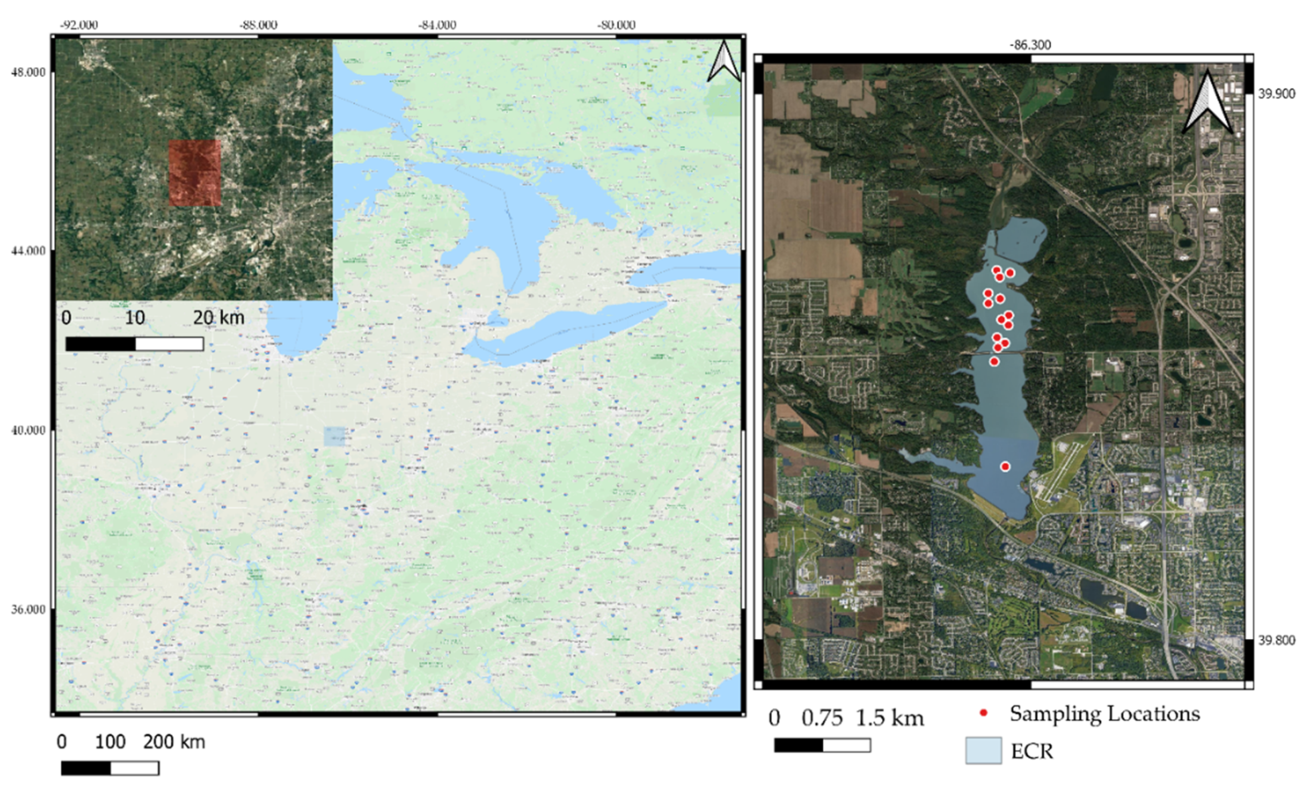
2.1. Study Site and Sampling

The site of this study was Eagle Creek Reservoir (ECR, 86°18′13.07″ W, 39°51′09.84″ N) with a surface area of 5.0 km2 and a mean water depth of 4.2 m (Figure 1). ECR is one of the major drinking and recreational water systems in the Indianapolis metropolitan, Indiana USA. In ECR, cyanobacteria blooms have been recurrent in the last years with the predominance of Planktothrix rubescens, Planktothrix agardhii, and Pseudanabaena catenata [14]. ECR has a seasonal thermal stratification from June to September. Reservoir mixing usually occurs in April/May and October each year. To capture this thermal stratification, 24 field campaigns were conducted in ECR from April to October 2018. For each field campaign, the same sampling locations (Figure 1) were visited for collection of radiometric and limnological variables.

2.2. Algal Pigments Concentration

Water samples were collected just below the water surface at each sampling station (Figure 1). Water samples were stored on ice in coolers until the samples were shipped back to the laboratory where water samples were filtered and frozen immediately to prevent pigment denaturalization. Chlorophyll-a (chl-a) concentration was estimated based on the EPA Method 446.0, in which chl-a was extracted from the frozen glass fiber filters (GF/F, Whatman, GE Healthcare Life Sciences Whatman, Buckinghamshire, UK) with 90% acetone [15]. The final concentration was calculated from spectrophotometrically readings of the extracted solution following Jeffrey and Humphrey’s Trichromatic Equations [16]. Since there is no standard method for PC extraction, we used the current state-of-the-art procedures where PC was extracted from the frozen GF/F using a 50 mM phosphate buffer pH 6.8 and repeated freezing and thawing of cells [17]. The PC concentration was determined by fluorometrically readings of the extracted solution in a TD700 fluorometer (Turner Designs, Inc., Sunnyvale, CA, USA) equipped with a Cool White Mercury Vapor Lamp and a PC Optical Kit (630-nm excitation and 660-nm emission filters). Fluorometric measurements were calibrated using a set of dilutions of a C-phycocyanin standard (Sigma-Aldrich 52468, St. Louis, MO, USA). A total of 332 samples were collected and analyzed.

2.3. Proximal Remote Sensing Reflectance below the Water Surface (rrs) Acquisition

Proximal hyperspectral reflectance below the water surface (rrs) spectra were measured for the 14 sampling sites during the 24 field campaigns in the year of 2018 in the ECR. A total of 336 samples were measured using a dual head Ocean Optics USB4000 system composed of two spectroradiometers (351–1047 nm, 0.2-nm spectral resolution, and 3645 bands (Ocean Insight, Inc., Orlando, FL, USA). One spectroradiometer was mounted on a 2-m-high pole pointed upward to measure the downwelling irradiance (Ed), and simultaneously the other spectroradiometer equipped with a 25° field-of-view optical fiber, was dipped ~5 cm below the water surface via a 2-m-long pole to measure the below-surface upwelling radiance (Lu) at nadir. rrs was finally calculated following the procedure described by Gitelson et al. [18].

2.4. OLI’ Spectral Band Simulation

The simulation of OLI spectral bands was carried out using in situ rrs measurements and the spectral response function of OLI (f), using Equation (1) [19]. The spectral response function for the OLI spectral bands (including the PAN spectral band) were acquired from the Landsat 8 webpage (http://landsat.gsfc.nasa.gov/?p=5779 Accessed on 15 January 2022) whereas the spectral response function for the orange contra-band was acquired from Castagna et al. [11,12] which is available at the library within the ACOLITE—an atmospheric correction for aquatic systems using the “dark spectrum fitting” approach [20,21].
R r s , k = λ 1 k λ 2 k R r s ( λ , t ) S k ( λ ) d λ λ 1 k λ 2 k S k ( λ ) d λ
where Sk(λ) is the radiometric sensitivity of band k, whose band width is from wavelength λ1k to λ2k.
Since the spectral response function of the orange contra-band can only be calculated from hyperspectral measurements, Castagna et al. [12] proposed a semi-empirical relationship (Equation (2)) to estimate the orange contra-band using the PAN, green (centered at 561 nm) and red (centered at 655 nm) spectral bands. This relationship is important because it allows the computation of the orange contra-band from the OLI image without the need for a hyperspectral image.
To validate the proposed relationship (Equation (2)), we compared the simulated orange contra-band based on the spectral response function to the modeled orange contra-band based on the empirical relationship among the OLI spectral bands.
R r s ( o r a n g e ) = [ 2.2861   ( ± 0.1303 ) · R r s ( P A N ) ] [ 0.9467   ( ± 0.0611 ) · R r s ( g r e e n ) ] [ 0.1989   ( ± 0.0712 ) · R r s ( r e d ) ]
Additionally, we also established a relationship between the simulated orange contra-band based on the spectral response function and the modeled orange contra-band based on the empirical relationship among the OLI spectral bands. Our proposed relationship was computed using a multiple linear regression and the results were compared to the one proposed by Castagna et al. [20] (Equation (2)) using a Mann–Whitney Rank Sum Test to validate their proposed slopes.

2.5. PC Retrieval Assessment

For the retrieval of PC using Landsat 8/OLI simulated bands the following remote sensing algorithms were evaluated: (1) green:orange ratio, (2) OLH [20] and (3) orange:red ratio [13]. These remote sensing algorithms were calculated for the entire dataset; therefore, the assessment was based on the scatterplots, correlation coefficient (r), determination coefficient (R2) and root mean square error (RMSE).

3. Results

3.1. Orange Contra-Band

The multiple linear regression analysis using the PAN, the green and the red simulated spectral bands (Equation (3)) for all sampling points (n = 336) was used to estimate simulated orange contra-band based on the spectral response function.
R r s ( o r a n g e ) = [ 6.98 · 10 6 ] + [ 2.464 · R r s ( P A N ) ] [ 0.957 · R r s ( g r e e n ) ] [ 0.281 · R r s ( r e d ) ]
In comparison to the relationship proposed by Castagna et al. [12] (Equation (2)), the coefficient of each independent parameter in the multiple regression is larger even if a plus-one standard deviation was considered. However, the median value of the simulated orange contra-band for the empirical relationship proposed by Castagna et al. [12] was 0.00562 while our relationship (Equation (3)) showed a median value of the simulated orange contra-band as 0.00567. Additionally, a strong correlation was observed between the simulated orange contra-band based on the spectral response function and the modeled orange contra-band based on the empirical relationship (Equations (2) and (3)), with a r of 0.997 and a R2 of 0.994 (Figure 2A) for Castagna et al. [12] and a r of 0.998 and a R2 of 0.996 for the one proposed in this study (Figure 2B). Both relationships showed an RMSE lower than 0.001 showing very similar performances from both relationships. A Mann–Whitney Rank Sum Test showed that the difference in the median values between the two modeled Rrs orange is not statistically significant (p = 0.991). Therefore, these insignificantly small variations in empirical relationships (Equations (2) and (3)) validate the relationship proposed by Castagna et al. [20].

3.2. PC Retrieval from Simulated OLI Data

PC and chl-a concentrations measured for 332 samples collected in the ECR (Figure 1) during the year of 2018 were used to test different remote sensing models. The central tendency statistical estimators of both pigments showed that the range of PC during the year was larger than the range of chl-a and correspondingly, the standard deviation, the variance and the coefficient of variation were also higher for the PC (Table 1). Chl-a had a higher mean, median and 25 and 75 percentile values indicating that for most of the samples, chl-a was higher than PC concentration, despite the dramatically different maximum values for the two pigments. The PC concentration (in log scale) showed a weak relationship with remote sensing models using the entire dataset (n = 332, Figure 3), and low R2 values were found for the three remote sensing models tested: 0.02, <0.01 and 0.08 for the green:orange ratio, OLH, and orange:red ratio, respectively (Table 2).
To improve these relationships, we used only the samples with a PC concentration higher than 50 μg/L—which was described by Ruiz–Verdu et al. [22] as the optimal concentration for PC retrieval (Figure 4). The resultant R2 values were improved for the green:orange ratio (R2 = 0.16) and the OLH (R2 = 0.24) with a geometric fit, but decreased for the orange:red ratio with a logarithmic fit (R2 = <0.01). Overall, the use of PC concentration higher than 50 μg/L did not significantly improve the retrieval of PC. Nevertheless, it was observed that green/orange ratio performed slightly better than the other two models.
The retrieval of PC for samples with the PC:chl-a ratio higher than 1.5 (n = 35) was also performed considering that a high PC:chl-a ratio means the spectral dominance of PC over chl-a. In this way, an improvement on the retrieval of PC concentration (Figure 5) was observed. The green:orange ratio got a strong geometric relationship with a R2 of 0.84, while the OLH and orange:red models got R2 values of 0.33 and 0.45 respectively with a geometric fit. These values indicate that the retrieval of PC is possible, however, current remote sensing models can only do it when PC is the dominant pigment.

4. Discussion

4.1. Remote Sensing Models Evaluation

The performance of the three remote sensing models for estimating PC concentration in waters with mixed phytoplankton groups (Figure 3 and Figure 4) showed weaker correlation as described in previous research. Ogashawara [23] evaluated the use of Sentinel 3/OLCI for the estimation of PC concentration in Lake Erie and showed that the ratio between the Rrs at 681 and 620 got a R2 of 0.41 and the ratio green:orange was the best for the estimation of chl-a concentration on samples with concentrations higher than 50 μg/L (R2 = 0.88). In addition, in Lake Erie, USA, Kumar et al. [13] showed that for Landsat 8/OLI, the orange:red ratio got a R2 of 0.55 for a PC concentration range from 0.23 to 170.39 μg/L (n = 16). Additionally, in this same study the authors also evaluated the use of different remote sensing models for Sentinel 3/OLCI and obtained a R2 of 0.74 using the orange and red-edge spectral bands. OLH was also evaluated using an image over Lake Erie [12] based on the correlation between PC relative fluorescence unit and the OLH values. The stronger performance shown by these mentioned studies [12,13,23] could be attributed to the fact that these studies used Lake Erie as the study site. Lake Erie is the most productive lake among the Laurentian Great Lakes and has experienced intensifying cyanobacterial blooms in the past decade [24]. Additionally, the lake during summer months has been dominated by cyanobacteria species such as Microcystis, Planktothrix and Anabaena since 1995 [25,26]. The improved performance was also observed for the model tested in the current study when applied to of the samples with PC:chl-a ratio higher than 1.5 (Figure 5, Table 2), implying the interference of other optically active constituents on the tested remote sensing models.
Considering that Landsat 8/OLI bands have a low spectral resolution, a weak performance of the tested remote sensing models for PC retrieval is expected for non-cyanobacteria dominated waters because of the influence of other optically active constituents. For example, the influence of chl-a at 620 nm has been investigated by different studies [3,27,28]. Simis et al. [3] used an empirical factor (ε) to relate the in vivo absorption of chl-a at 665 nm to its absorption at 620 nm and corrected for the chl-a effect. Mishra et al. [27] proposed to determine the absorption coefficient of PC at 620 nm by use of two factors (ψ1 and ψ2) and the difference of the absorption coefficient of phytoplankton at 620 nm and the absorption coefficient of chl-a at 665 nm. Ogashawara and Li [28] proposed a new method to accommodate the contribution of chl-a absorption at 620 and PC at 665 nm. All three studies emphasized a significant contribution of chl-a absorption to the absorption coefficient at 620 nm. However, these studies used hyperspectral data with a 1-nm spectral resolution. Therefore, considering that Landsat 8/OLI bands are much wider—green (533–590 nm) and red (636–673 nm)—more interference from other optically active constituents are expected.
In the current state-of-the art, remote sensing algorithms for PC estimation with OLI imagery should be improved by removing the effect of other optically active constituents. There is a need for the development or tuning of new remote sensing models for Landsat 8/OLI bands, especially for the retrieval of PC from non-cyanobacteria dominated waters.

4.2. Importance of the Orange Contra-Band for Aquatic Systems

This study showed that the semi-empirical method proposed by Castagna et al. [12] for estimating the orange contra-band is very promising for high-resolution imaging in aquatic environments as indicated by statistically insignificant difference between the empirical orange contra-band and the semi-empirical method (Figure 2). Requiring the very specific absorption feature around 620 nm [1,3,5,28], the estimation of PC has been limited to the imagery acquired by MERIS or OLCI sensors. However, these sensors have a low spatial resolution (300 m), and are not suitable for monitoring small to medium aquatic systems. Verpoorter et al. [29] reported that waterbodies with an area smaller or equals to 1 km2 comprise 60% of the total surface area of global inland waters. Although these small aquatic systems are large enough to occupy more than one single pixel at a spatial resolution of 300 m, the interference from the adjacent pixels on the signal of the pixel under consideration would be very strong [12]. The adjacency effect in aquatic systems is usually observed around the near-infrared spectral region which is caused by the effect of the reflected skylight or surrounding land in the water surface [30]. Ogashawara et al. [31] showed that only a few atmospheric correction routines were able to remove the adjacency effect for small to medium lakes in Germany for Landsat 8/OLI images. Considering the spatial resolution, it would be improbable to have a reliable estimation of PC from most inland aquatic systems using a 300 m spatial resolution image
The orange contra-band generation with Landsat satellite multispectral data can complement the existing satellite-based monitoring of water quality which are usually sparse in space and time, and site-specific [32], especially for tracking cyanobacterial blooms to address public concern about the drinking water safety [33,34]. While traditional water quality monitoring uses data from few points within an aquatic system the use of the orange contra-band could allow the monitoring of the entire water surface. This would improve the monitoring of the areas which are not sampled, for example, the areas close to the shoreline which are usually used for leisure activities. However, as demonstrated in this study, the use of the orange contra-band is only accurate when PC is the dominant pigment. Therefore, more research is needed on the accurate retrieval of PC from Landsat satellite imagery for aquatic systems where PC is not the dominant pigment which is important for the tracking the development of a CHABs and consequently forecasting it.

5. Conclusions

This study validated the proposed approach for the computation of the OLI’s orange contra-band [11,12] and its potential for PC estimation using three different remote sensing models. The simulated and calculated orange contra-band showed a significant correlation, and the proposed semi-empirical method by [12] performed well for the samples from ECR. Additionally, this study evaluated the performance of three remote sensing models for the retrieval of PC concentrations. While all three remote sensing algorithms failed to estimate PC concentration from water different optical water types, their performance was improved when only PC dominant waters were evaluated. These results highlighted the need for the development or tuning of remote sensing models for the accurate estimation of PC concentration from non-cyanobacteria dominant waters to serve as a monitoring tool for water quality managers. Considering that ECR as well as several other small to medium sized aquatic systems are used for water supply purposes, the development of such tools are important. The need for these tools is pressing as CHABs are known to produce neurotoxins and hepatotoxins which are related to diseases such as Dementia, Alzheimer’s and other neurological impairments, and liver and kidney failure [34]. Thus, the orange contra-band generation of Landsat 8/OLI opens a new era for the use of Landsat 8/OLI to estimate PC. Thus, the environmental need for the monitoring of CHABs are promising for the development of an environmental health monitoring program which could be used by policy makers to assess water quality for water supply and recreational uses.

Author Contributions

Conceptualization, I.O. and L.L.; methodology, I.O. and L.L.; software, I.O.; validation, I.O., C.H.; formal analysis, I.O.; investigation, I.O., L.L., C.H. and G.K.D.; resources, G.K.D. and L.L.; data curation, I.O.; writing—original draft preparation, I.O.; writing—review and editing, I.O., L.L., C.H. and G.K.D.; visualization, I.O.; supervision, G.K.D. and L.L.; project administration, G.K.D. and L.L.; funding acquisition, G.K.D. All authors have read and agreed to the published version of the manuscript.

Funding

This research was funded by Citizen Energy Group.

Institutional Review Board Statement

Not applicable.

Informed Consent Statement

Not applicable.

Data Availability Statement

The data presented in this study are available on request from the corresponding author.

Acknowledgments

In this section, you can acknowledge any support given which is not covered by the author contribution or funding sections. This may include administrative and technical support, or donations in kind (e.g., materials used for experiments).

Conflicts of Interest

The authors declare no conflict of interest.

References

  1. Dekker, A.G. Detection of the Optical Water Quality Parameters for Eutrophic Waters by High Resolution Remote Sensing. Ph.D. Thesis, Free University, Amsterdam, The Netherlands, 1993. [Google Scholar]
  2. Schalles, J.F.; Yacobi, Y.Z. Remote detection and seasonal patterns of phycocyanin, carotenoid and chlorophyll pigments in eutrophic waters. Arch. Hydobiol. Spec. Issues Advanc. Limnol. 2000, 55, 153–168. [Google Scholar]
  3. Simis, S.G.H.; Peters, S.W.M.; Gons, H.J. Remote sensing of the cyanobacterial pigment phycocyanin in turbid inland water. Limnol. Oceanogr. 2005, 50, 237–245. [Google Scholar] [CrossRef]
  4. Mishra, S.; Mishra, D.R.; Schluchter, W.M. A novel algorithm for predicting phycocyanin concentrations in cyanobacteria: A proximal hyperspectral remote sensing approach. Remote Sens. 2009, 1, 758–775. [Google Scholar] [CrossRef] [Green Version]
  5. Li, L.; Sengpiel, R.E.; Pascual, D.L.; Tedesco, L.P.; Wilson, J.S.; Soyeux, A. Using hyperspectral remote sensing to estimate chlorophyll-a and phycocyanin in a mesotrophic reservoir. Int. J. Remote Sens. 2010, 31, 4147–4162. [Google Scholar] [CrossRef]
  6. Ogashawara, I.; Mishra, D.R.; Mishra, S.; Curtarelli, M.P.; Stech, J.L. A performance review of reflectance based algorithms for predicting phycocyanin concentrations in inland waters. Remote Sens. 2013, 5, 4774–4798. [Google Scholar] [CrossRef] [Green Version]
  7. Gregor, J.; Maršálek, B.; Šípková, H. Detection and estimation of potentially toxic cyanobacteria in raw water at the drinking water treatment plant by in vivo fluorescence method. Water Res. 2007, 41, 228–234. [Google Scholar] [CrossRef]
  8. Catherine, A.; Escoffier, N.; Belhocine, A.; Nasri, A.B.; Hamlaoui, S.; Yéprémian, C.; Bernard, C.; Troussellier, M. On the use of the FluoroProbe®, a phytoplankton quantification method based on fluorescence excitation spectra for large-scale surveys of lakes and reservoirs. Water Res. 2012, 46, 1771–1784. [Google Scholar] [CrossRef]
  9. Riddick, C.A.L.; Hunter, P.D.; Domínguez Gómez, J.A.; Martinez-Vicente, V.; Présing, M.; Horváth, H.; Kovács, A.W.; Vörös, L.; Zsigmond, E.; Tyler, A.N. Optimal cyanobacterial pigment retrieval from ocean colour sensors in a highly turbid, optically complex lake. Remote Sens. 2019, 11, 1613. [Google Scholar] [CrossRef] [Green Version]
  10. Donlon, C.; Berruti, B.; Buongiorno, A.; Ferreira, M.H.; Féménias, P.; Frerick, J.; Goryl, P.; Klein, U.; Laur, H.; Mavrocordatos, C.; et al. The Global Monitoring for Environment and Security (GMES) Sentinel-3 mission. Remote Sens. Environ. 2012, 120, 37–57. [Google Scholar] [CrossRef]
  11. Castagna, A.; Simis, S.; Dierssen, H.; Vanhellemont, Q.; Sabbe, K.; Vyverman, W. Extending the operational land imager/landsat 8 for inland water research: Retrieval of an orange band from pan and ms bands. In Proceedings of the Ocean Optics Conference (Ocean Optics XXIV), Dubrovnik, Croatia, 7–12 October 2018. [Google Scholar]
  12. Castagna, A.; Simis, S.; Dierssen, H.; Vanhellemont, Q.; Sabbe, K.; Vyverman, W. Extending landsat 8: Retrieval of an orange contra-band for inland water quality applications. Remote Sens. 2020, 12, 637. [Google Scholar] [CrossRef] [Green Version]
  13. Kumar, A.; Mishra, D.R.; Ilango, N. Landsat 8 virtual orange band for mapping cyanobacterial blooms. Remote Sens. 2020, 12, 868. [Google Scholar] [CrossRef] [Green Version]
  14. Tedesco, L.; Clercin, N. Algal ecology, cyanobacteria toxicity and secondary metabolites production of the three eutrophic drinking water supply and recreational use reservoirs in central Indiana. In Veolia Water Research Project Final Report; CEES: Indianapolis, IN, USA, 2010; pp. 25–29. [Google Scholar]
  15. Arar, E.J. In vitro determination of chlorophylls a, b, c1 + c2 and pheopigments in marine and freshwater algae by visible spectrophotometry. In USEPA Method 446.0.; EPA: Washington, DC, USA, 1997; pp. 1–26. [Google Scholar]
  16. Jeffrey, S.W.; Humphrey, G.F. New Spectrophotometric Equation for Determining Chlorophyll A, B, C1 and C2. Biochem. Physiol. Pflanz 1975, 167, 194–204. [Google Scholar] [CrossRef]
  17. Sarada, R.; Pillai, M.G.; Ravishankar, G.A. Phycocyanin from Spirulina sp: Influence of processing of biomass on phycocyanin yield, analysis of efficacy of extraction methods and stability studies on phycocyanin. Process Biochem. 1999, 34, 795–801. [Google Scholar] [CrossRef]
  18. Gitelson, A.A.; Schalles, J.F.; Hladik, C.M. Remote chlorophyll-a retrieval in turbid, productive estuaries: Chesapeake Bay case study. Remote Sens. Environ. 2007, 109, 464–472. [Google Scholar] [CrossRef]
  19. van der Meer, F. Physical principles of optical remote sensing. In Spatial Statistics for Remote Sensing; Stein, A., van der Meer, F., Gorte, B., Eds.; Kluwer Academic Publishers: Dordrecht, the Netherlands, 1999. [Google Scholar]
  20. Vanhellemont, Q.; Ruddick, K. Atmospheric correction of metre-scale optical satellite data for inland and coastal water applications. Remote Sens. Environ. 2018, 216, 586–597. [Google Scholar] [CrossRef]
  21. Vanhellemont, Q. Adaptation of the dark spectrum fitting atmospheric correction for aquatic applications of the Landsat and Sentinel-2 archives Remote Sens. Environ. 2019, 225, 175–192. [Google Scholar]
  22. Ruiz-Verdú, A.; Simis, S.G.H.; de Hoyos, C.; Gons, H.J.; Peña-Martínez, R. An evaluation of algorithms for the remote sensing of cyanobacterial biomass. Remote Sens. Environ. 2008, 112, 3996–4008. [Google Scholar] [CrossRef]
  23. Ogashawara, I. The use of sentinel-3 imagery to monitor cyanobacterial blooms. Environments 2019, 6, 60. [Google Scholar] [CrossRef] [Green Version]
  24. Allinger, L.E.; Reavie, E.D. The ecological history of Lake Erie as recorded by the phytoplankton community. J. Great Lakes Res. 2013, 39, 365–382. [Google Scholar] [CrossRef]
  25. Harke, M.J.; Davis, T.W.; Watson, S.B.; Gobler, C.J. Nutrient-Controlled Niche Differentiation of Western Lake Erie Cyanobacterial Populations Revealed via Metatranscriptomic Surveys. Environ. Sci. Technol. 2016, 50, 604–615. [Google Scholar] [CrossRef] [PubMed]
  26. Steffen, M.M.; Davis, T.W.; McKay, R.M.L.; Bullerjahn, G.S.; Krausfeldt, L.E.; Stough, J.M.A.; Neitzey, M.L.; Gilbert, N.E.; Boyer, G.L.; Johengen, T.H.; et al. Ecophysiological Examination of the Lake Erie Microcystis Bloom in 2014: Linkages between Biology and the Water Supply Shutdown of Toledo, OH. Environ. Sci. Technol. 2017, 51, 6745–6755. [Google Scholar] [CrossRef] [PubMed]
  27. Mishra, S.; Mishra, D.R.; Lee, Z.; Tucker, C.S. Quantifying cyanobacterial phycocyanin concentration in turbid productive waters: A quasi-analytical approach. Remote Sens. Environ. 2013, 133, 141–151. [Google Scholar] [CrossRef]
  28. Ogashawara, I.; Li, L. Removal of chlorophyll-a spectral interference for improved phycocyanin estimation from remote sensing reflectance. Remote Sens. 2019, 11, 1764. [Google Scholar] [CrossRef] [Green Version]
  29. Verpoorter, C.; Kutser, T.; Seekell, D.A.; Tranvik, L.J. A global inventory of lakes based on high-resolution satellite imagery. Geophys. Res. Lett. 2014, 41, 6396–6402. [Google Scholar] [CrossRef]
  30. Odermatt, D.; Kiselev, S.; Heege, T.; Kneubuhler, M.; Itten, K.I. Adjacency effect consideration and air/water constituent retrieval for Lake Constance. In Proceedings of the 2nd MERIS/(A)ATSR Workshop, Frascati, Italy, 22–26 September 2008; Lacoste, H., Ouwehand, L., Eds.; ESA-ESRIN: Frascati, Italy, 2018. [Google Scholar]
  31. Ogashawara, I.; Jechow, A.; Kiel, C.; Kohnert, K.; Berger, S.A.; Wollrab, S. Performance of the Landsat 8 provisional aquatic reflectance product for inland waters. Remote Sens. 2020, 12, 2410. [Google Scholar] [CrossRef]
  32. Michalak, A.M. Study role of climate change in extreme threats to water quality. Nature 2016, 535, 349–350. [Google Scholar] [CrossRef]
  33. Schaeffer, B.A.; Schaeffer, K.G.; Keith, D.; Lunetta, R.S.; Conmy, R.; Gould, R.W. Barriers to adopting satellite remote sensing for water quality management. Int. J. Remote Sens. 2013, 34, 7534–7544. [Google Scholar] [CrossRef]
  34. Clark, J.M.; Schaeffer, B.A.; Darling, J.A.; Urquhart, E.A.; Johnston, J.M.; Ignatius, A.R.; Myer, M.H.; Loftin, K.A.; Werdell, P.J.; Stumpf, R.P. Satellite monitoring of cyanobacterial harmful algal bloom frequency in recreational waters and drinking water sources. Ecol. Indic. 2017, 80, 84–95. [Google Scholar] [CrossRef] [PubMed]
Figure 1. Location of ECR and sampling points used in this study.
Environments 09 00040 g001
Figure 2. (A) Relationship between modeled Rrs (orange) and True Rrs (orange) based on the Castagna et al. [12] relationship (Equation (2)); and (B) Relationship between modeled Rrs (orange) and True Rrs (orange) based on multiple linear regression (Equation (3)).
Environments 09 00040 g002
Figure 3. PC concentration (in log scale) and remote sensing models relationship using the entire dataset (n = 332). (A) for the green:orange ratio; (B) for the OLH; and (C) for the orange:red ratio.
Environments 09 00040 g003
Figure 4. PC concentration (in log scale) and remote sensing models relationship using only the data in which PC concentration was higher than 50 μg/L (n = 72). (A) for the green:orange ratio; (B) for the OLH; and (C) for the orange:red ratio.
Environments 09 00040 g004
Figure 5. Correlation between PC concentration and remote sensing parameters for the samples with PC:chl-a ratios higher than 1.5 (n = 35). (A) for the green:orange ratio; (B) for the OLH; and (C) for the orange:red ratio.
Environments 09 00040 g005
Table 1. Statistical summary for the PC and chl-a concentrations in ECR during the year of 2018.
PC (μg/L)Chl-a (μg/L)
Minimum8.366.26
Maximum290.33123.23
Mean40.6148.76
Variance1956.69535.77
Standard Deviation44.2323.14
Median21.2345.82
25 percentile15.3232.65
75 percentile43.8663.75
Coefficient of Variation108.9247.46
Table 2. Best fit for each remote sensing model for each dataset.
Best FitR2DFp-Value
Green:orange—n = 332Linear0.023301
OLH—n = 332Geometric<0.013301
Orange:red—n = 332Geometric0.083301
Green:orange—n = 72Geometric0.1670<0.001
OLH—n = 72Geometric0.2470<0.001
Orange:red—n = 72Logarithmic<0.01700.579
Green:orange—n = 35Geometric0.8433<0.001
OLH—n = 35Geometric0.3333<0.001
Orange:red—n = 35Geometric0.5433<0.001
Publisher’s Note: MDPI stays neutral with regard to jurisdictional claims in published maps and institutional affiliations.

