Article

Spontaneous Plants Improve the Inter-Row Soil Fertility in a Citrus Orchard but Nitrogen Lacks to Boost Organic Carbon

by
Fernando Visconti
1,2,*,
Enrique Peiró
1,
Carlos Baixauli
3 and
José Miguel de Paz
1
1
Instituto Valenciano de Investigaciones Agrarias-IVIA, Centro para el Desarrollo de la Agricultura Sostenible-CDAS, Carretera CV-315, km 10.7, 46113 Moncada, Valencia, Spain
2
Departamento de Ecología, Centro de Investigaciones Sobre Desertificación-CIDE (CSIC, UVEG, GVA), Carretera CV-315, km 10.7, 46113 Moncada, Valencia, Spain
3
Fundación Cajamar, Centro de Experiencias Cajamar, Camino del Cementerio Nuevo, s/n, 46200 Paiporta, Valencia, Spain
*
Author to whom correspondence should be addressed.
Environments 2022, 9(12), 151; https://doi.org/10.3390/environments9120151
Submission received: 2 November 2022 / Revised: 21 November 2022 / Accepted: 29 November 2022 / Published: 4 December 2022
(This article belongs to the Special Issue Soil Organic Carbon Assessment)

Abstract

:
The inter-row soils in conventionally run citrus orchards in Eastern Spain lose fertility, either physically, chemically, or biologically, as a consequence of machinery traffic and the use of herbicides. In order to regain inter-row soil fertility, two grass-cover management alternatives to the commonly used herbicide-kept bare management, namely, spontaneous plants and fescue, were established and left for four years until their effects on several physical, chemical, and biological parameters were monitored for two years more. The fescue ground cover exhibited lower average and maximum soil temperatures due to higher evapotranspiration rates but also higher annual soil water content on average and, additionally, higher rhizodeposition. Despite the fact that these new beneficial conditions helped enhance the soil’s biological fertility under fescue, the physical or chemical fertilities did not improve and neither did the organic carbon (SOC). The spontaneous plants also enhanced the biological fertility, but in this case, beneficial conditions were reflected by improvements in the chemical fertility, particularly the exchangeable potassium, and in the physical fertility by increasing the surface hydraulic conductivity and decreasing the bulk density. In the inter-rows of this citrus orchard, a seeded grass cover does not seem able to provide any soil fertility enhancement in comparison to a spontaneous one; rather the opposite. However, a lack of natural or man-driven nitrogen inputs poses a constraint to SOC gains. For this aim, the annual surface application of organic nitrogen-rich materials or even better, the fostering of N-fixing organisms would be recommended.

1. Introduction

In agriculture, soil fertility is the soil’s ability to provide crops with a favorable environment where they can optimally develop and yield. Soil fertility is made up of interdependent chemical, physical, and biological factors [1,2]. The soil’s chemical fertility is the soil’s ability to provide crops with the amounts of nutrients their genetic potential requires as readily absorbable ions and molecules. The soil’s physical fertility is the soil’s ability to provide crops with a porous ground material that their roots can explore to anchor to and obtain oxygen, water, and nutrients at the pace that these are required according to the plants’ growth and weather conditions. Finally, the soil’s biological fertility is the soil’s ability to provide crops with a community of overall mutualistic organisms, i.e., ones that help plants to obtain the oxygen, water, and nutrients their roots look for, with no harm induced by competition, parasitism, or (micro)predation.
Nowadays, conventional agriculture is characterized as follows. It tries to maximize soil chemical fertility through the application of synthetic fertilizers that exceed the crop’s needs. It tries to maintain the soil’s physical fertility, often by means of harsh tillage operations, e.g., moldboard plowing. Finally, it constrains the soil’s biological fertility to the control of competing organisms, parasites, and plant (micro)predators by using tillage and/or xenobiotic chemicals. All of these practices ignore the interdependence among chemical, physical, and biological fertility and thus lead to land degradation [3,4,5,6]. In addition, in the case of drip irrigation systems, the need for fertility is only circumscribed to the emitter-dampened soil volume. Lastly, considering the inter-rows as little more than alleyways for machinery traffic further damages soil fertility [7].
In Spain, there is currently 5,340,000 ha with woody crops, among which 307,000 ha, i.e., ≈6%, are with citrus, over half in the Valencian Community (Eastern Spain) [8]. Spanish citrus soils are mostly drip irrigated (≈84%) [8] and subjected to herbicide applications for weed control (≈75%) [9]. Conventionally managed Spanish citrus soils not only feature low organic carbon [10,11] but also high bulk density because of the constant agricultural machinery traffic on the inter-rows [12]. The soil compaction experienced by citrus soils under conventional management practices harms their physical fertility, which appear as decreased topsoil water infiltration [13] and, as a consequence, higher runoff and erosion rates [12,14].
High compaction is strongly related to low soil organic carbon (SOC) [15,16,17,18], and therefore, the deterioration of physical fertility worsens chemical fertility. Fortunately, the converse has been observed, as ameliorating one fertility aspect improves the other and vice versa [19,20]. In this regard, there are several soil-management practices that may be applied to the inter-rows of citrus plantations so as to increase their SOC and decrease their compaction, e.g., the use of cover crops [21] including spontaneous plants and mulching with agricultural by-products such as rice straw [22].
These management practices, especially cover crops, improve the soil’s chemical fertility by increasing SOC, and the soil’s physical fertility by increasing porosity, water infiltration, available water capacity, and structural stability. Additionally, they improve the soil’s biological fertility in woody crop orchards (i) by increasing enzyme activity [23,24,25], (ii) controlling weeds [26,27], and by controlling harmful insects [28], therefore becoming an alternative to the use of xenobiotic chemicals.
Among cover crops, seeded ones, either with Poaceae or Leguminosae or mixtures of both, are the standard [29]. However, since they are genuine crops, they have to be cultivated, which includes seeding, cutting, and even watering and fertilizing [30]. This way, they become an expense to the farmer. The question is whether they make up for this expense in terms of soil fertility and SOC increase and, moreover, how they compare with spontaneous plants, which due to their nature, are more easily managed.
To the best of our knowledge, in citrus orchards, the alternative inter-row soil management of spontaneous plants has not been compared against the conservative treatment using Poaceae cover crops and conventional bare-soil treatment by means of herbicide application. In the framework of the soil and climate conditions of the citrus orchards from the Valencian coastal plain (Eastern Spain), the tested hypothesis is that in the short-to-medium term, the use of grass cover crops, specifically, spontaneous plants, on the inter-rows, enhances the soil’s physical, chemical, and biological fertility more than keeping the soil bare.

2. Materials and Methods
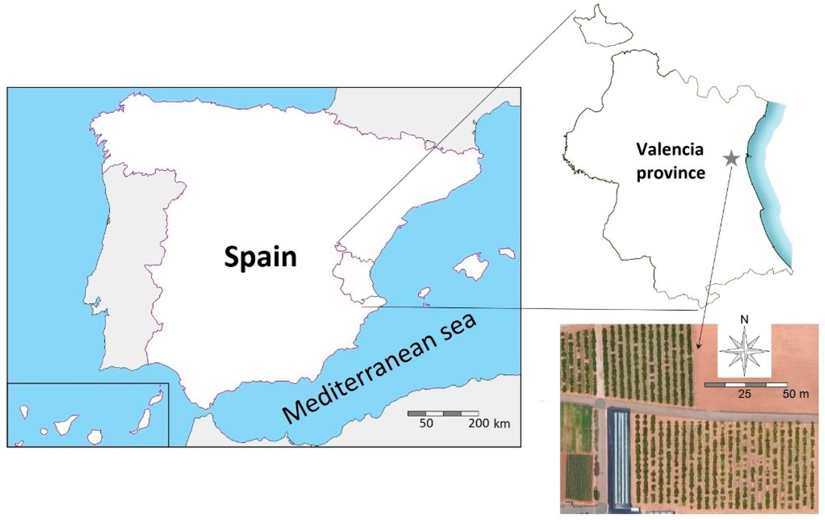
2.1. Study Site

A citrus orchard located at the Centro de Experiencias Cajamar in the municipality of Paiporta (coordinates 39°25′2″ N, 0°25′4″ W, altitude of 17 m, slope < 1%) was selected as the study site (Figure 1). This emplacement is at the bottom of a Pleistocene accumulation piedmont immediately contiguous to the Valencian coastal plain. The climate of the area is semiarid hot-summer Mediterranean (Csa), according to the Köppen–Geiger classification [31], and the soils are Typic calcixerepts, according to the Soil Taxonomy [32].

2.2. Crop and Irrigation Characteristics

The site was planted between 2013 and 2014 with clementine (Citrus clementina) grafted onto Cytrange carrizo with a 5 × 2 m2 spacing, and the irrigation system was trickle on the tree lines with a double hose per plant row. Fertigation was carried out according to the usual practices in the surrounding Valencia area.

2.3. Treatments and Trial Plots

Three management methods for the soil on the inter-rows were set up as treatments with two trial plots that were 10-to-15-m-long per each one: (i) the soil kept bare as a control using weed killers (bare), (ii) the soil left with no weed control (spontaneous), and (iii) the soil planted with fescue (Festuca spp.) as a cover crop (fescue). Both the establishment and maintenance of these treatments are described in some detail below.
In the control treatment, a broad-spectrum herbicide (glyphosate) plus minor quantities of other more weed-specific herbicides, following the conventional practices in the citrus production of the Valencia area, were applied to keep the soil bare throughout the experiment time stretch. Before the winter of 2015, the soil under all treatments had been subjected to this same treatment with herbicides. From the winter of 2015 onwards, the soil on the inter-rows in the spontaneous treatment was left to freely grow local weeds, whereas, in the fescue treatment, the grass was sown.
Following the setup of the treatments, all plants on the inter-row, either sowed or spontaneous, were reaped on a regular basis each spring, summer, and winter. Importantly, the residues were not mixed with the soil but left on it. The rest of the agricultural operations were the same in all treatments. Furthermore, no other fertilizers or management practices different from the ones just described were applied to the inter-rows. Starting from the winter–spring of 2019, the trials were monitored for two years.

2.4. Weather Measurements

Rainfall was measured with an ECRN-50 (METER Group, Inc., Pullman, WA, USA) rain gauge installed at a 1 m height in a clear spot near the center of the study site, and the data were recorded by means of a ZL6 m (METER Group, Inc., Pullman, WA, USA). The atmospheric pressure (P) data were measured and saved by means of one ZL6 m per treatment. The air temperature and relative humidity were measured and recorded with one HOBO MX2301 (Onset Computer Corp., 470, Bourne, MA, USA) installed at a 1 m height in the middle of one trial plot per treatment.

2.5. Soil Measurements and Samplings

All of the soil measurements and samplings were performed on the inter-rows, avoiding the areas near the drip emitters.

2.6. Soil Temperature and Water Content Measurements

For the monitoring of the soil temperature and water content, two 5TM (METER Group, Inc., Pullman, WA, USA) capacitance probes per trial plot were installed between 5 and 10 cm depths.

2.7. Soil Saturated Hydraulic Conductivity

The soil-surface saturated hydraulic conductivity (Ks) was assessed by using a single-ring infiltrometer with a 12.5 cm diameter and a 6.5 cm height, filled with water with a 400 μS/cm electrical conductivity at 25 °C [33]. Two batches of Ks measurements composed of four repetitions per trial plot were made, one at the beginning and another at the end of the monitoring.
During each infiltration measurement, a constant hydraulic head (H) of 1 cm was kept on the soil surface and the cumulative infiltration values (I) were taken against time (t) for 20 min. In order to calculate Ks, first of all, it was determined from which time the infiltration rate reached a steady state. This minimum time to reach steadiness in water infiltration (tmin) was determined in the laboratory through the visual inspection of the I against t graph and calculation of the coefficient of determination (R2) of the following equation:
I = a f Ks t + c
where a is a dimensionless constant with a 0.9084 value, c is an empirical parameter, and f is a geometric parameter that depends on the hydraulic head and the single-ring dimensions according to:
f = 1 + (H + 12.5)/(d + r/2)
where d is the depth of the ring insertion and r is its radius [34]. Once tmin was known, Equation (1) was considered to represent the water infiltration into the soil from there onwards, and Ks can be assessed from its slope.

2.8. Soil Carbon Dioxide Emission Rate

Polyvinyl chloride (PVC) collars of 10 and 4.5 cm in, respectively, inner radius (r) and height, were driven 3.5 cm into the soil in two places across the inter-row of each trial plot and left for the entire project time span. Then, the soil CO2 emission was measured once every one or two months in the collar-delimited areas.
To measure the soil CO2 emission rate every time it was made, a measurement chamber was constructed over the PVC collars by tightly fitting a steel cylinder with a 10 cm outer radius and a 16 cm height and a PVC cover on top. This lid was equipped with a K-30 (SenseAir AB, Delsbo, Sweden) dispersive infrared CO2 sensor and, additionally, an HS-2000V (Kele Precision Manufacturing, Memphis, TN, USA) air temperature (T) and relative humidity (RH) sensor.
The chamber cover was connected by means of a multi-wire cable to an Arduino UNO (Smart Projects S.R.L., Scarmagno, Italy) microcontroller, which was also connected to a real-time clock (RTC), a 16 × 2 liquid crystal display (LCD), a 4 GB secure digital (SD) card recorder, and a 12 V battery. A program in the C language was written in the Arduino Development Environment (ADE) and loaded into the microcontroller to take measurements in the chamber headspace of the CO2 volumetric fraction (xCO2), T and RH every five seconds for 30 min.
In order to calculate the soil C-CO2 emissions, firstly, the C-CO2 volumetric mass content in the chamber (ρC-CO2) was calculated from the xCO2, T, and P data according to the following equation:
ρ C - CO 2 = x CO 2 M C P R ( T + 273.15 )
where MC is the C molar mass and R is the gas constant. Then, a polynomial was tried to fit the data of ρC-CO2 against time (t), and, in general, a fourth-degree one was found to be quite representative of the C-CO2 evolution in the chamber:
ρC-CO2 = α + βt + γt2 + δt3 + εt4
The polynomial coefficients were estimated by means of least squares fitting. Since covering the soil with a closed measurement chamber is known to alter the previous natural flux of soil CO2 [35], a pre-deployment soil C-CO2 emission rate per unit surface (EC-CO2) was estimated from the derivative of Equation (4) at t = 0 [36]. This initial rate equals the β coefficient in Equation (4), and thus, the EC-CO2 was estimated by multiplying the β coefficient in Equation (4) by the chamber height (h):
EC-CO2 = β h

2.9. Undisturbed Soil Sampling for Bulk Density

Undisturbed soil core samples with a 5 cm diameter and height were taken using steel cylinders and a 0753SA (Eijkelkamp, Giesbeek, The Netherlands) volumetric sampler at two depth intervals: 0–5 and 20–25 cm. During the experiment, three batches of core samples from three points per trial plot were collected.
These core samples of known volume (V) were hermetically closed in the field and, once in the laboratory, dried at 105 °C for 24 h and weighed (mss). Then, the soil was extracted from the cylinders and disaggregated. The coarse fragments (>2 mm) were separated and weighed to find their mass (mcf), whereas their volume (Vcf) was estimated assuming a standard particle density of 2.65 g cm−3 and applying Vcf = mcf/2.65. Then, the apparent density of the fine earth (<2 mm) (ρb) was calculated by means of:
ρb = (mssmcf)/(VVcf)

2.10. Undisturbed Soil Sampling for Roots

Using the aforementioned volumetric equipment, undisturbed core samples were taken in four points per trial plot but only at a 0–5 cm depth for the root-weight mass fraction assessment only once during the experiment time span. The core samples were again hermetically closed, and once in the laboratory, they were weighed to find the field soil mass (mfs). Then, the soil was extracted from the steel cylinders, and one rootless sub-sample per core was taken, weighed, dried at 105 °C for 24 h, then reweighed to assess the gravimetric field water mass fraction (wfs), and finally, the dry mass of the whole undisturbed soil (mds) was calculated. The roots were separated from the rest of the soil by sieving and flotation, dried at 65 °C for 48 h, and weighed to find their mass (mroot). Then, the mass fraction of the roots in the soil (wroot) was calculated by using this equation:
wroot = mroot/mds

2.11. Disturbed Soil Sampling

Disturbed soil samples were also taken with a steel sampling tube. Following sampling, the extracted soil material was thoroughly mixed, and one subsample was separated, transferred to a plastic pot, and kept in an ice chest at 5–10 °C, whereas the rest of the sample was simply sealed in a plastic bag and kept at air temperature. Three places per trial plot were drilled every three months throughout the experiment at depths of 0–20 cm. However, at the beginning of the experiment, the 20–40 and 40–60 cm layers were also sampled.
Once in the laboratory, the low-temperature-preserved subsamples were kept at 4 °C until the field water content, dehydrogenase activity (DHA), and β-D-glucosidase (GLA) activity could be determined. The field water content was determined by oven-drying a subsample at 105 °C for 24 h, whereas DHA and GLA were determined according to the methods of, respectively, Casida et al. [37] and Tabatabai and Bremner [38].
The non-refrigerated soil was spread onto polyethylene trays, which were bottom-covered with ashless filter paper sheets and left to air-dry. Then, the hygroscopic water content was determined by oven-drying a subsample at 105 °C for 24 h. The soil nitrogen mass fraction (wN) was determined using the Kjeldahl method [39]. The SOC mass fraction (wSOC) was determined by the Walkley–Black method [40] using 1.33 as the Walkley–Black coefficient [41]. The available soil phosphorus (wP) was estimated using the Olsen–Watanabe method [42]. The extractable potassium (nK) was determined by displacement with 1 N ammonium acetate and measurement by emission flame spectrophotometry. Finally, texture, according to the USDA, was assessed using a Bouyoucos densimeter [43].

2.12. Statistical Analyses

Before the comparisons among treatments, each batch of data was analyzed to ascertain if it satisfactorily fulfilled the requirements of normality. The adjusted Fisher–Pearson standardized moment coefficient (G1) and the Kolmogorov–Smirnov test were used to assess normality. In case this could not be accepted, then a logarithm to base 10 or even a square root transformation were tried in this order, and the G1 and the Kolmogorov–Smirnov test were reassessed. Then, Pearson’s product–moment correlation coefficients among all of the normalized variables were calculated by using the mean values of each season and subplot. Next, it was ascertained if the variables significantly changed among the soil treatments by means of two-way ANOVAs, where an additional variable, i.e., sampling or measurement time, was included along with the treatments. Regarding this, if the interaction between the treatment and sampling or measurement time could be considered significant, then as many one-way ANOVAs as sampling or measurement times were carried out instead. Two-way ANOVA and, if necessary, one-way ANOVAs for each sampling or measurement time, were followed by orthogonal comparisons, in which the following a priori hypotheses were tested: (i) the joint bare and spontaneous treatments against the fescue and (ii) the bare soil against the spontaneous plants. In this work, a p-value below 0.05 has been regarded as revealing significant differences, and all average values have been expressed as the arithmetic mean plus its 95% confidence interval according to the Student’s t distribution.

3. Results

3.1. General Observations

The soil in the study site is not stony (mcf/mss < 2%), clay loam, and moderately calcareous (Table 1). In addition, at the beginning of the monitoring in the bare inter-rows, the soil was also found to be poor in organic matter and moderately compacted (Table 1). In the spontaneous treatment, the soil covering attained between 50 and 90% in spring due to a mixture of, primarily, false barley (Hordeum murinum) and, secondarily, horseweed (Conyza canadensis), whereas soil covering decreased to between 10 and 20% in winter, summer, and autumn when the horseweed dominated. The fescue treatment attained a more homogeneous soil covering, which ranged between 60 and 80%.

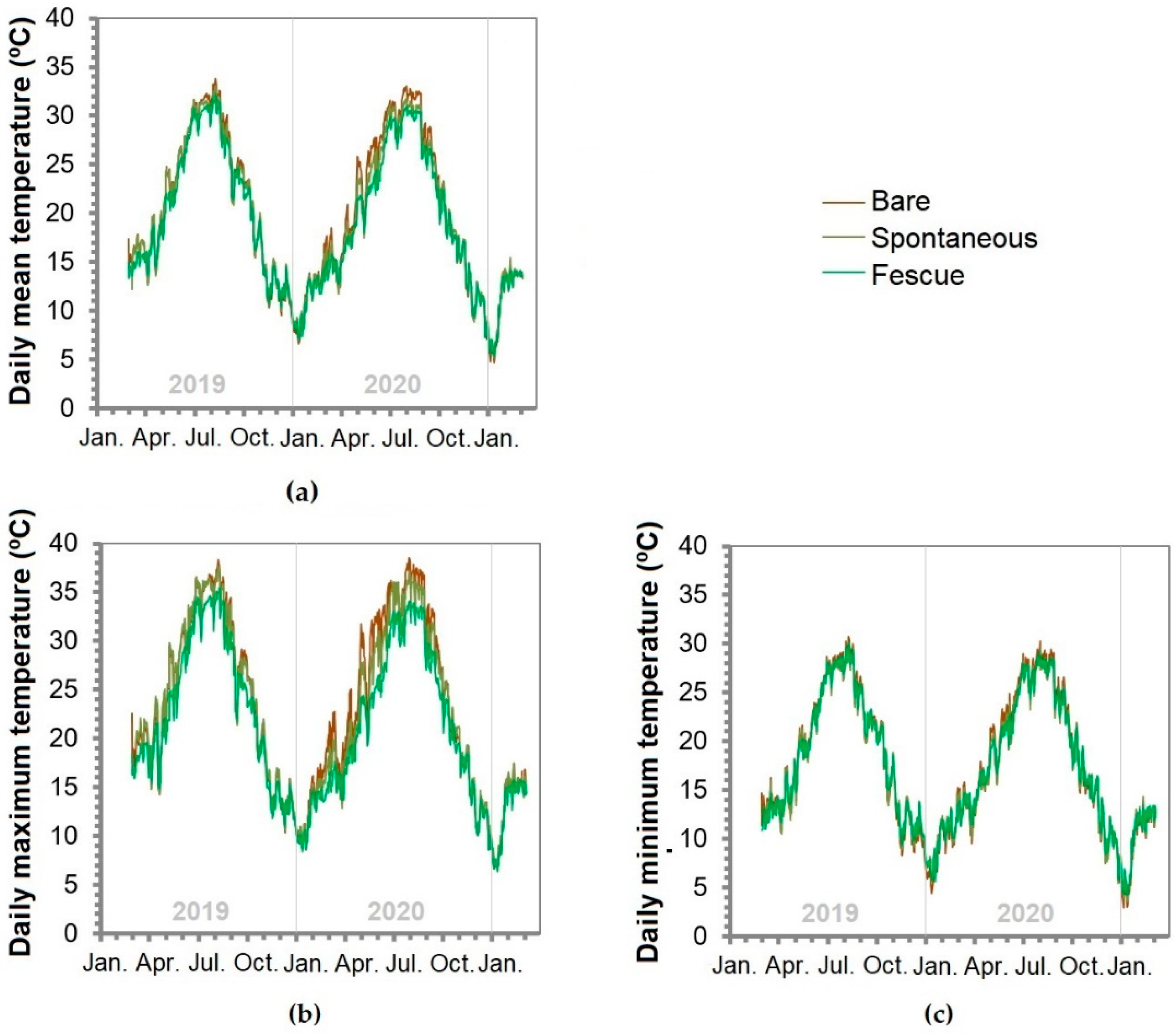
3.2. Soil Temperature

The differences in soil temperature between the treatments were remarkable. The mean daily temperature was the lowest under fescue with 19.1 ± 0.3 °C whereas the spontaneous plants and bare soil had the highest with a joint of 19.8 ± 0.2 °C. Therefore, the treatments may be arranged in the following order from lower to higher soil temperature: fescue < spontaneous plants ≈ bare soil.
As can be seen in Figure 2, the differences in mean daily temperature among the treatments were primarily caused by the differences in maximum daily temperature and not by the differences in the minimum one. Specifically, the maximum mean daily temperature was again the lowest under fescue at 21.1 ± 0.3 °C, and then, under the spontaneous plants and bare soil, which again featured the highest with a joint of 22.8 ± 0.2 °C. Contrary to the maximum temperature, there were no differences in the minimum mean daily temperature between the treatments, and a joint of 17.5 ± 0.1 °C could be calculated for all three.

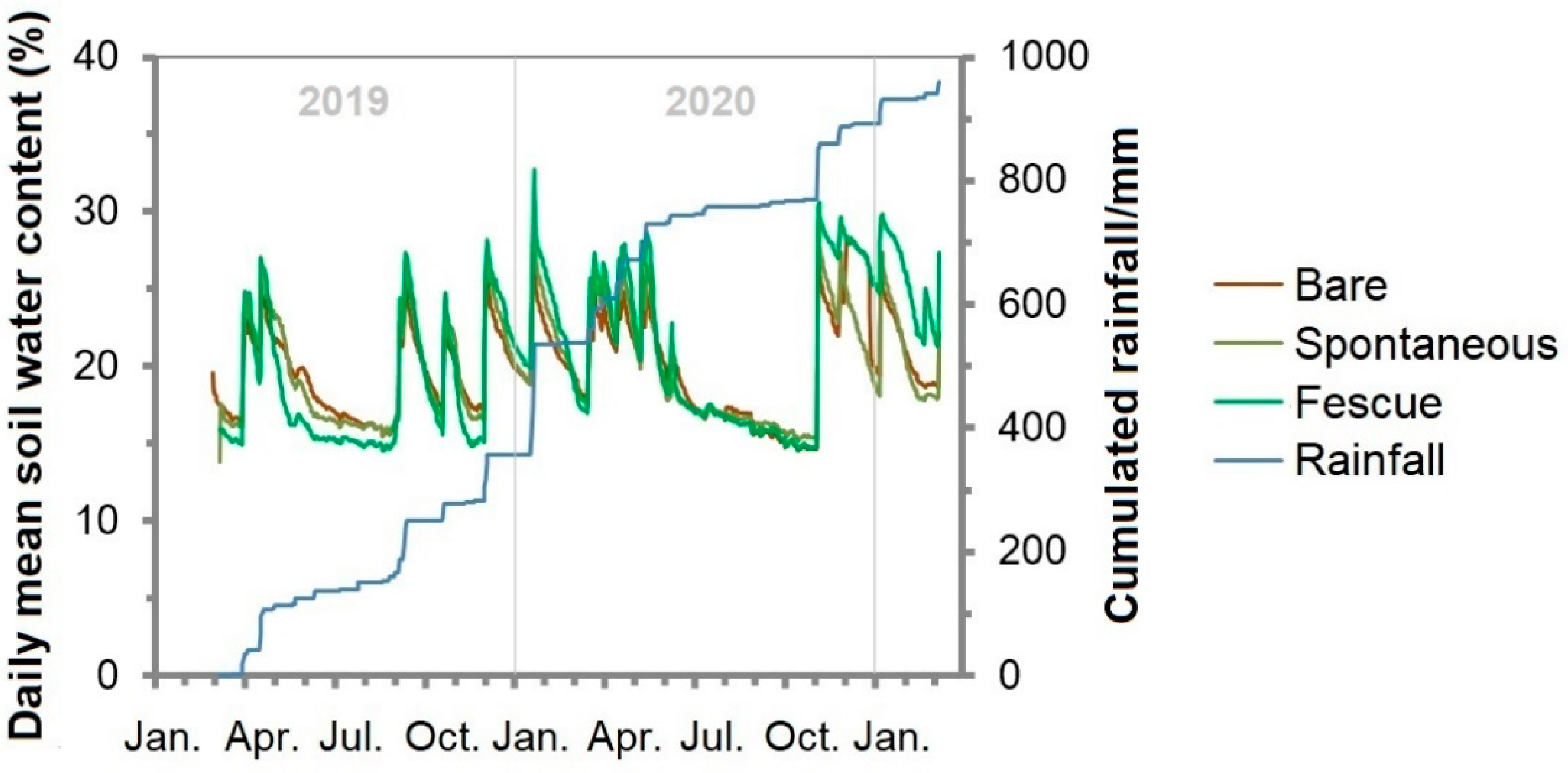
3.3. Soil Water Content

In addition to temperature, there were also remarkable differences in the soil water content between the treatments. The mean daily water content was the lowest in both the bare soil and spontaneous plants, which had a joint of 0.199 ± 0.001, followed by the fescue with 0.205 ± 0.002. Therefore, the treatments may be arranged in the following order from lower to higher annual average water content: bare soil ≈ spontaneous plants < fescue. This order reverses the soil temperature one. Notwithstanding this, the fescue left the soil drier than the other treatments during spring and, particularly, summer, likely because of the plant evapotranspiration during those seasons (Figure 3).

3.4. Statistical Characteristics of the Soil Properties

The general statistical features of the soil variables were evaluated (Table S1). Additionally, the adjusted Fisher–Pearson standardized moment coefficient (G1) and the Kolmogorov–Smirnov test parameters were calculated (i) to assess the normality of their distributions and (ii) to study the adequate transformation to attain normality.
The saturated hydraulic conductivity data presented a G1 coefficient equal to 1.5, which means that Ks followed a distribution with a heavy tail to the right, which, notwithstanding, could be accepted as normal according to the Kolmogorov–Smirnov test (p = 0.45) (Table S1). However, a logarithm-to-base-10 transformation led to a G1 very close to zero, specifically −0.1, and a p-value for the Kolmogorov–Smirnov test of 0.82 (Table S1). Therefore, the log Ks data were used for the statistical analyses instead of Ks.
The bulk density (ρb) data presented a G1 coefficient equal to −0.4, which means that ρb followed a distribution with no heavy tails, that could be accepted to come from a normal-like distribution according to the Kolmogorov–Smirnov test (p = 0.83) (Table S1). Therefore, the ρb data could be used with no transformation for the ensuing statistical analyses.
The soil root mass fraction (wroot) data presented a G1 coefficient equal to 2.4, which means that this property followed a distribution with a very heavy tail to the right that significantly departed from normality according to the Kolmogorov–Smirnov test (p = 0.027) (Table S1). A logarithm-to-base-10 transformation failed to fulfill both the G1 and the Kolmogorov–Smirnov normality criteria, and neither satisfactorily could a square root transformation. However, this last one, i.e., wroot1/2, with a G1 equal to 1.3 and a p-value of 0.11 for the Kolmogorov–Smirnov test (Table S1), was finally used for the statistical analyses instead of wroot.
The dehydrogenase activity (DHA) data presented a G1 coefficient equal to 1.4, which means that it followed a distribution with a remarkable tail to the right (Table S1). Although the non-normality was not corroborated by the Kolmogorov–Smirnov test (p = 0.22), the logarithm to base 10 transformation was tried, and it led to a more normal-like distribution, with a G1 coefficient equal to −0.5 and a p-value for the Kolmogorov–Smirnov test of 0.63 (Table S1). Therefore, the log DHA data were used for the statistical analyses instead of the DHA data.
The β-D-glucosidase activity (GLA) data presented a G1 coefficient equal to 1.3, which means that the GLA followed a distribution with a remarkable tail to the right, which, according to the Kolmogorov–Smirnov test, significantly departed from normality (p = 0.015) (Table S1). A logarithm-to-base-10 transformation led to a G1 equal to 0.05 that did not depart from normality (p = 0.83) (Table S1). Therefore, the log GLA data were used for the statistical analyses instead of the GLA data.
The soil C-CO2 emission (EC-CO2) data presented a G1 coefficient equal to 2.7, which means that the EC-CO2 data followed a distribution with a very heavy tail to the right that did not fulfill the requirements for normality according to the Kolmogorov–Smirnov test (p < 0.001) (Table S1). A logarithm-to-base-10 transformation led to a G1 equal to −0.8 that did fulfill the requirements for normality according to the Kolmogorov–Smirnov test (p = 0.64) (Table S1). Therefore, the log EC-CO2 data were used instead of the EC-CO2 for the statistical analyses.
The soil organic carbon mass fraction (wSOC) data presented a G1 coefficient equal to −0.04, which means that the wSOC followed a distribution with no tails to the right or left that could be accepted as normal according to the Kolmogorov–Smirnov test (p = 0.25) (Table S1). Therefore, the wSOC data as such were used for the statistical analyses.
The soil nitrogen mass fraction (wN) data presented a G1 coefficient equal to 1.3, which means that wN followed a distribution with a remarkable tail to the right that could not be accepted as coming from a normally distributed population according to the Kolmogorov–Smirnov test (p = 0.003) (Table S1). A logarithm-to-base-10 transformation was tried, and the log wN data presented a G1 coefficient equal to 0.77, which according to the Kolmogorov–Smirnov test could be accepted to come from a normal-like distribution (p = 0.03) (Table S1). Therefore, the log wN data were used instead of the wN for the statistical analyses.
The soil extractable potassium (nK) data presented a G1 coefficient equal to 3.0, which means that the nK followed a distribution with a very heavy tail to the right that did not fulfill the requirements for normality according to the Kolmogorov–Smirnov test (p < 0.001) (Table S1). A logarithm-to-base-10 transformation led to a G1 equal to 1.50 that characterizes a distribution with a heavy tail to the right. However, according to the Kolmogorov–Smirnov test, the normality of this distribution was closes to normal (p = 0.022, Table S1), and, therefore, the log nK data were used instead of the nK for the statistical analyses.
The available soil phosphorus mass fraction (wP) data presented a G1 coefficient equal to 0.41, which means that wP has a slight tail to the right that was not heavy enough to make the wP data depart from the normality according to the Kolmogorov–Smirnov test (p = 0.81) (Table S1). Therefore, the data analyses were carried out with the wP data.

3.5. Associations among the Soil Properties

The associations among the variables were revealed by Pearson’s product–moment correlation coefficients that were found to be significantly different from zero, at least at the 95% confidence level. These were 11 out of 66, i.e., 17% (Table 2).
The association between T and θw featured a significant r of −0.65, which was driven by the annual Mediterranean weather cycle in which, particularly, the hottest and driest season match, i.e., summer. Additionally, wN and DHA were significantly correlated with T and θw, with the r between 0.42 and 0.67 in absolute value.
The wroot was expected to be associated with T and θw and with the nutrient contents and enzymatic activities. These expectations were partially fulfilled since wroot exhibited high correlations with θw, ρb, GLA and wP, and wN. However, r was only significant with wN since the scarce data that were collected for wroot prevented its correlation coefficients from attaining statistical significance regardless of their high values.
Remarkably, wSOC was not significantly associated with any other soil variable, featuring correlation coefficients between 0.02 and 0.27 in absolute value. Besides, neither DHA nor GLA were associated, thus suggesting that these two enzymatic activities take account of two independent aspects of the metabolism of the soil organisms. Interestingly, however, EC-CO2 was found to be significantly associated with GLA but not DHA. Finally, another relevant and expected association was found between ρb and Ks, which featured an r of −0.77.

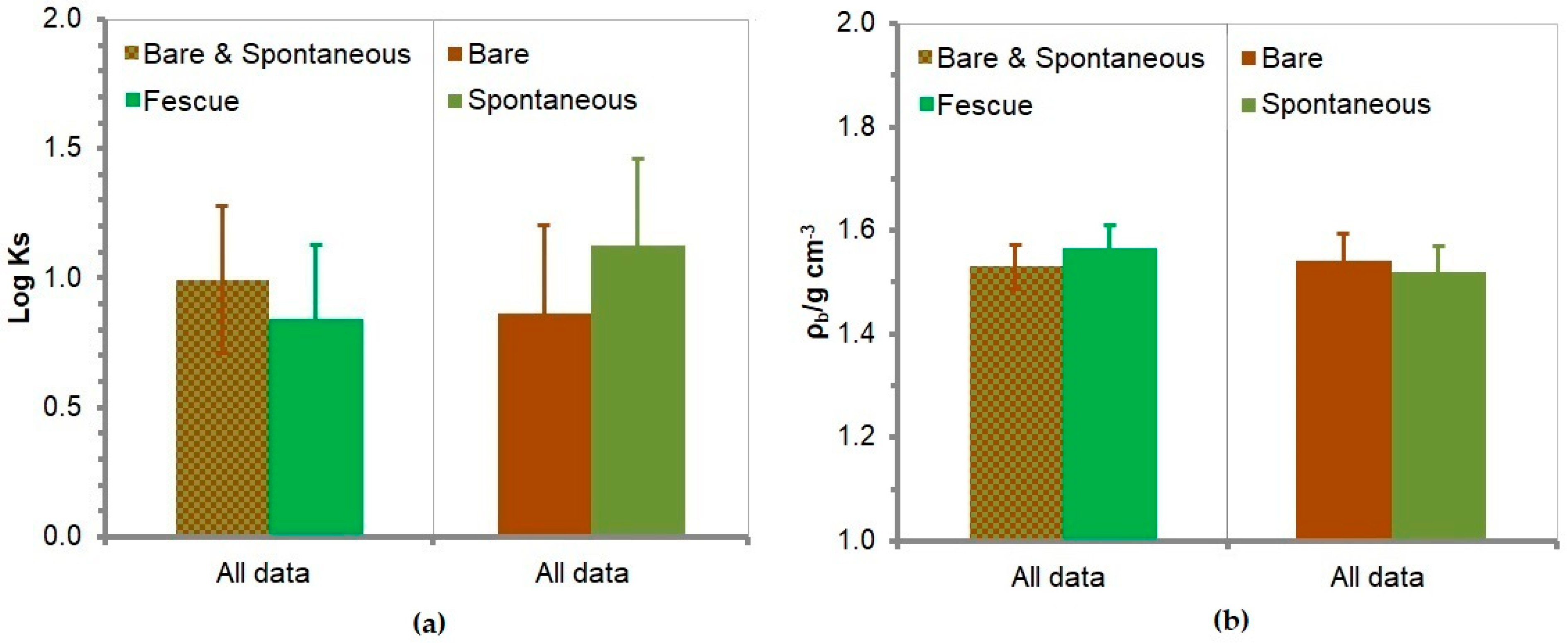
3.6. Soil Saturated Hydraulic Conductivity

According to the two-way ANOVA (Table 3), in general, the soil treatment did not have a significant effect on log Ks, but the measurement time did drop the Ks from spring 2019 to autumn 2020 (p = 0.03). However, since the effect of the soil treatments did not change in magnitude or direction from the first measurement to the second according to the non-significant interaction effect (p = 0.69, Table 3), the orthogonal contrasts among the soil treatments could be assessed on the basis of the two-way ANOVA results. As a consequence, it was found that between the combined bare soil and spontaneous plants, on the one hand, and fescue, on the other, there were no significant differences of log Ks at all (p = 0.28) (Figure 4), but that more remarkable differences, though still non-significant, appeared between bare soil and spontaneous plants (p = 0.12) with spontaneous on top.

3.7. Soil Bulk Density

According to the two-way ANOVA (Table 3), in general, the soil treatment did not have any significant effect on ρb, but again the sampling time did (p = 0.02). In addition, since, again, there were no significant changes in the magnitude or direction of the effect of the treatments on ρb from one sampling to the other according to the non-significant interaction (p = 0.33), the orthogonal contrasts were subsequently performed using all data. As a consequence, it was found that the combined bare and spontaneous treatments featured somewhat lower ρb than fescue, though non-significantly (p = 0.10) (Figure 4). Regarding the differences of ρb between bare and spontaneous, they were non-significant at all (p = 0.39). Note that these differences of ρb among treatments inversely reflect the ones obtained for log Ks (Figure 4). This result reveals the association between both physical fertility properties, which already showed up in the correlation analysis (Table 2).

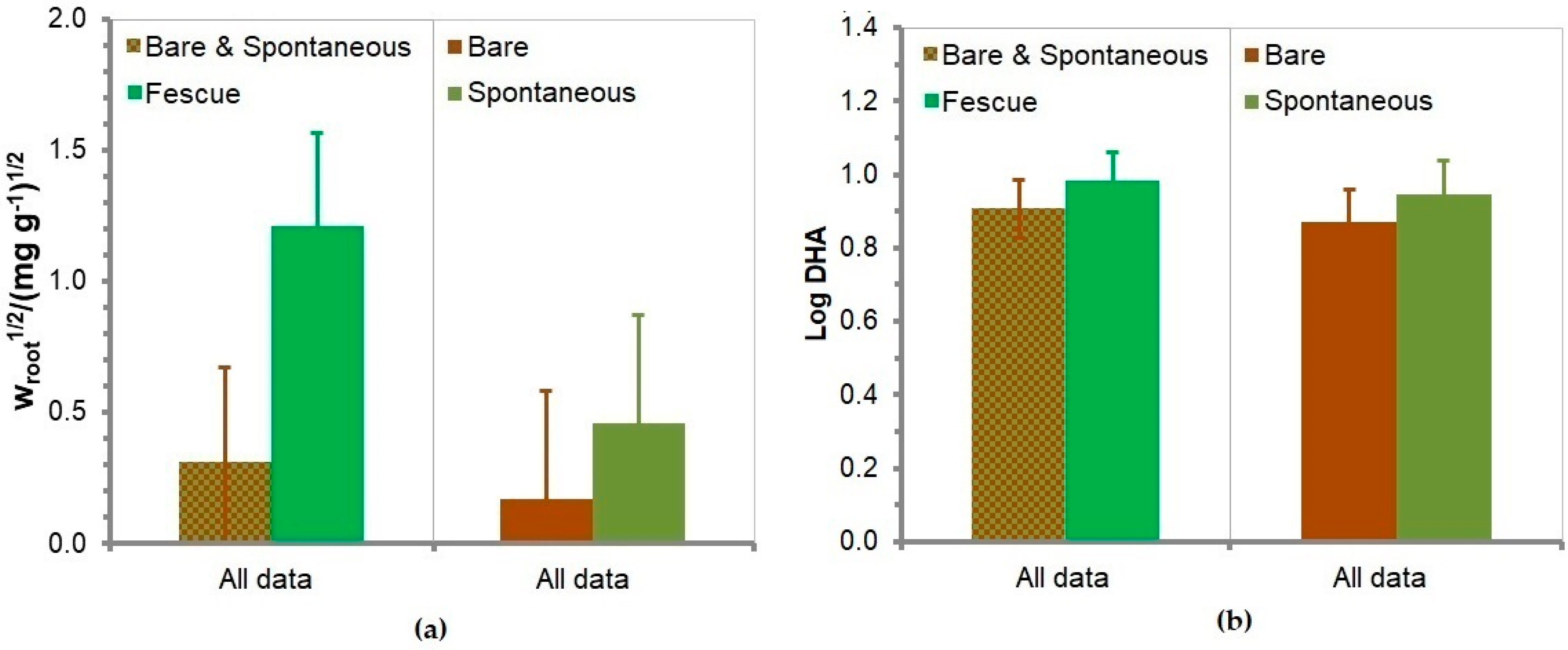
3.8. Soil Root Mass Fraction

According to the ANOVA (Table 3), there were very significant differences among the treatments (p < 0.001). Then, since only data for one measurement time were available, the orthogonal contrasts were readily assessed. As a consequence, it was found that the combined bare and spontaneous treatments featured significantly lower soil root mass than fescue (p < 0.001) and that there were no significant differences between bare soil and spontaneous plants (p = 0.15) (Figure 5).

3.9. Soil Dehydrogenase Activity

According to the two-way ANOVA (Table 3), the most significant differences were among the different seasons (p < 0.001) and then among the soil treatments (p = 0.045). However, since the effect of the treatments did not change in magnitude or direction from one season to the other according to the non-significant interaction effect (p = 0.50), the orthogonal contrasts among the soil treatments were assessed on the basis of all data. As a consequence, it was found that between the combined bare soil and spontaneous plants, on the one hand, and fescue, on the other, there were no significant differences in DHA for a narrow margin (p = 0.06) and that there were even fewer differences between bare soil and spontaneous plants (p = 0.10) (Figure 5). Note that these differences in DHA among treatments smoothly reflect the ones obtained for the wroot (Figure 5), which is in accordance with the dim association between DHA and wroot, as seen in the correlation analysis (Table 2).

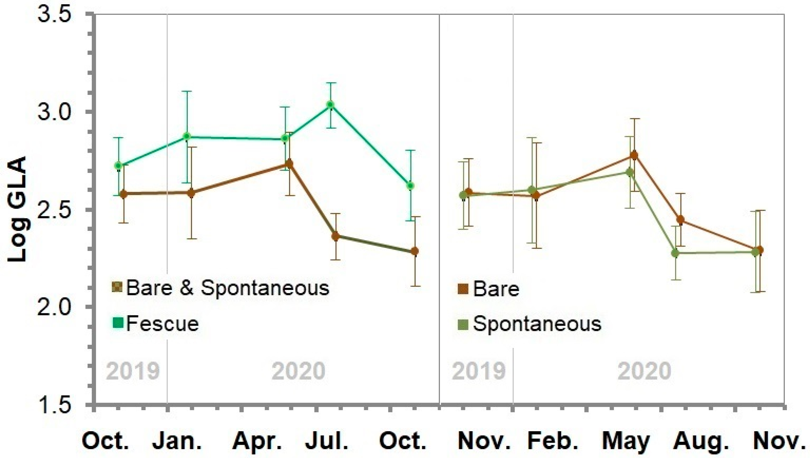
3.10. Soil β-D-Glucosidase Activity

According to the two-way ANOVA (Table 3), there were highly significant differences among the different soil treatments (p < 0.001) and sampling times (p < 0.001). Additionally, the effects of the soil treatments changed from one sampling to the other (p < 0.001). According to this significant interaction between the soil treatment and sampling time, five one-way ANOVAs and five batches of orthogonal contrasts, one per sampling time, were carried out. As a consequence, it was found that the combined bare and spontaneous treatments featured significantly lower GLA than fescue (p < 0.05) three out of five times. Conversely, there were non-significant differences in GLA between the bare soil and spontaneous plants (Figure 6).

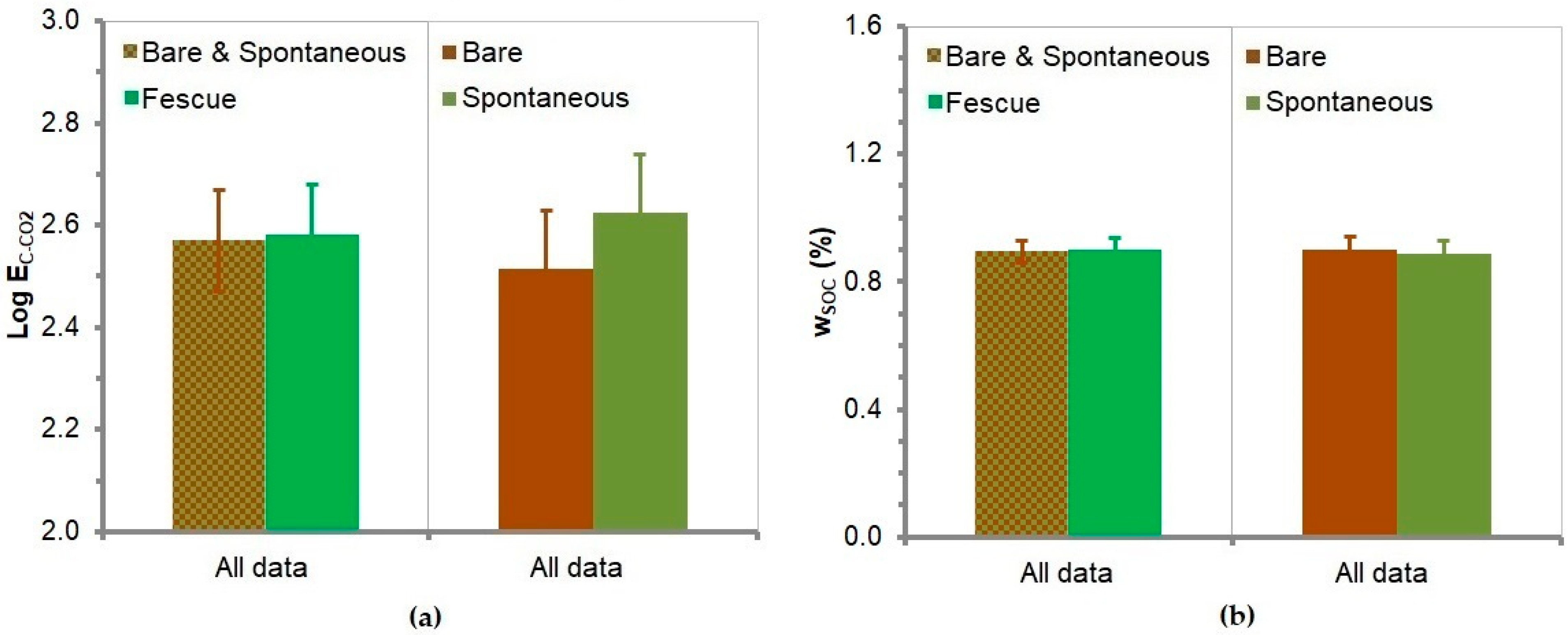
3.11. Soil Carbon Dioxide Emission

According to the two-way ANOVA (Table 3), there were significant differences among the measurement times (p < 0.001) but not among the treatments (p = 0.17), and the measurement time effects neither changed in magnitude nor direction from one treatment to the other according to the non-significant interaction effect (p = 0.19). According to this negligible interaction effect, and regardless of the non-significant treatment effects, the orthogonal contrasts among the soil treatments were assessed. As a consequence, it was found that between the combined bare soil and spontaneous plants, on the one hand, and fescue, on the other, there were no significant differences in EC-CO2 at all (p = 0.82) (Figure 7). However, the EC-CO2 in the spontaneous plants’ soil was higher than in the bare soil, though non-significantly by a very narrow margin (p = 0.06) (Figure 7).

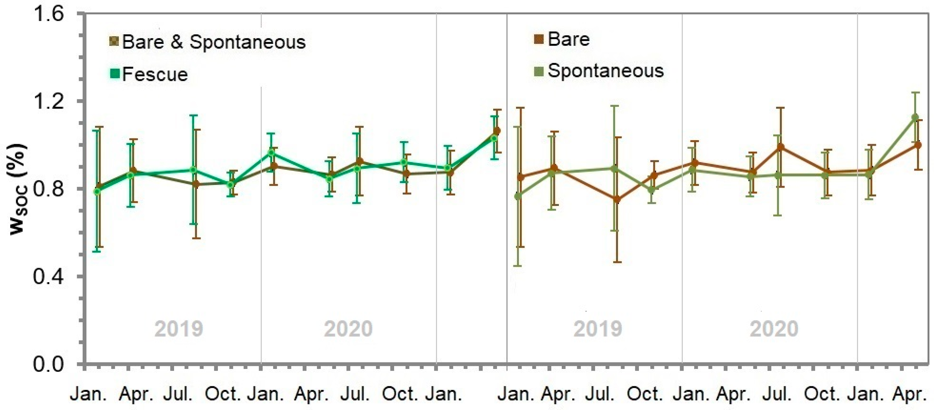
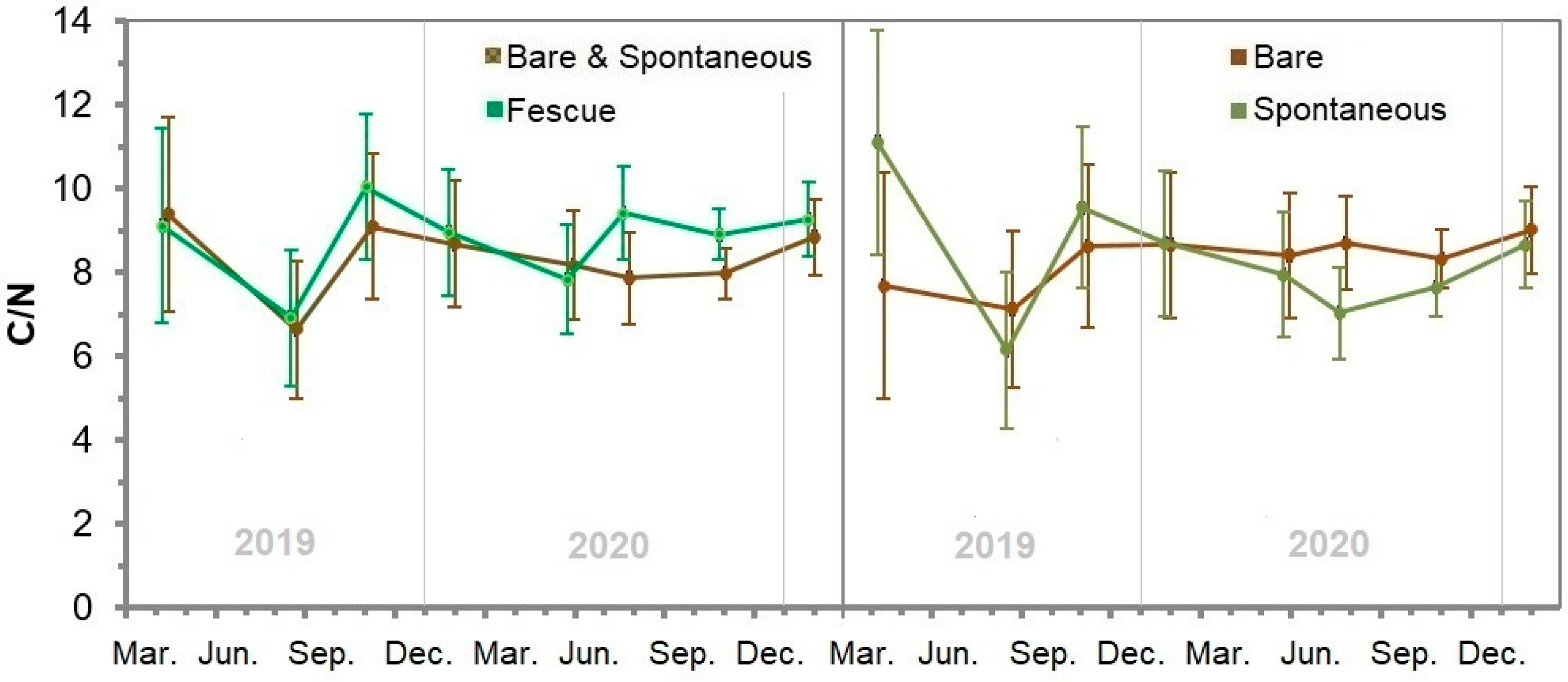
3.12. Soil Organic Carbon
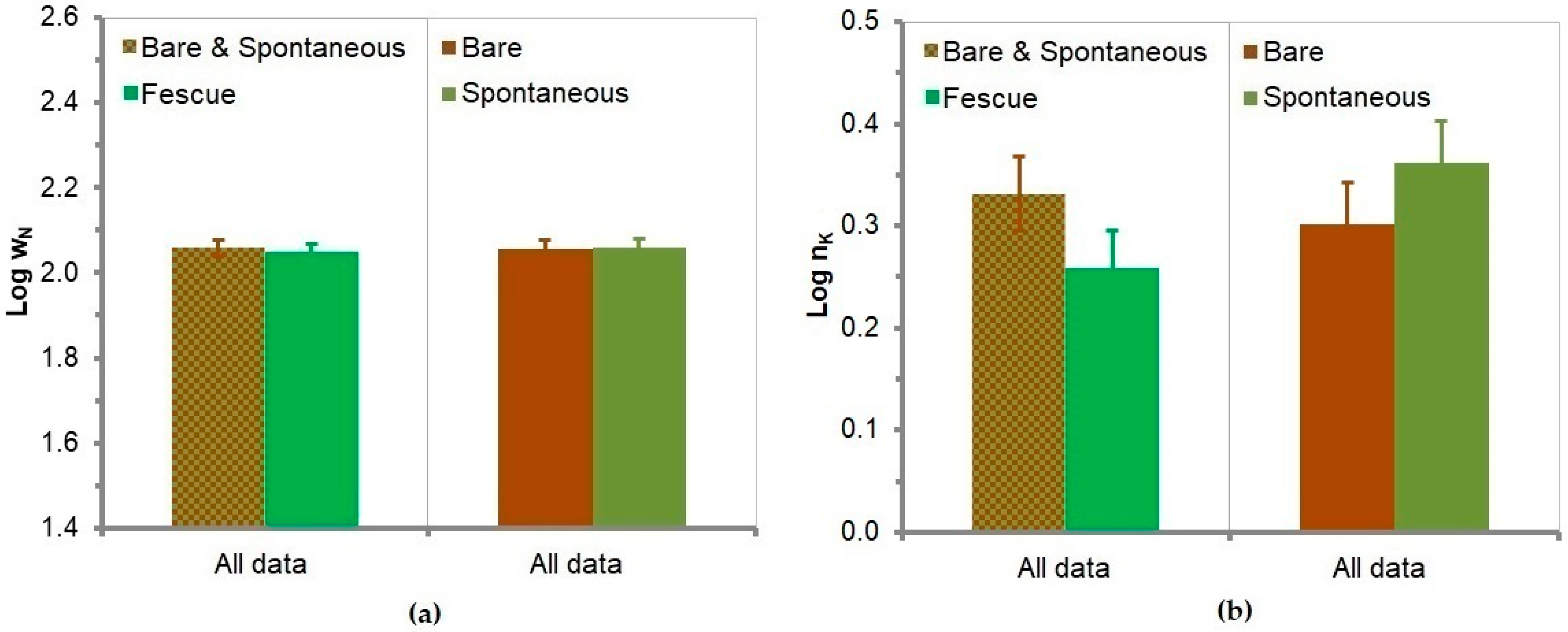
According to the two-way ANOVA (Table 3), there were highly significant differences among the different sampling times (p < 0.001) but not among the soil treatments (p < 0.77); additionally, the effect of the sampling time did not change from one treatment to the other (p = 0.35). According to this negligible interaction effect, and regardless of the non-significant treatment effects, the orthogonal contrasts among the soil treatments were assessed. As a consequence, it was found that the combined bare and spontaneous treatments featured the same wSOC as the fescue (p = 0.68) and that no wSOC differences existed between bare and spontaneous (p = 0.55) (Figure 7). Notwithstanding, some effects throughout time were discovered that eventually led to higher wSOC (Figure 8).

3.13. Soil Nitrogen

According to the two-way ANOVA (Table 3), there were highly significant differences among the different sampling times (p < 0.001) but not among the soil treatments (p = 0.60). This strong dependence of wN upon time may be driven by the root cycle throughout the year, as suggested by the high and significant correlations among wroot1/2, the weather cycle variables, i.e., T and θw, and wN (Table 2). Additionally, on the basis of the non-significant interaction (p = 0.11) between the treatments and sampling times found in the two-way ANOVA (Table 3), it was shown that the magnitude or direction of the treatments’ effects did not change from one sampling time to the other. According to this negligible interaction, the orthogonal contrasts among the soil treatments were assessed to graphically put forth the absence of significant differences between all three treatments (Figure 9).
Related to soil organic carbon and nitrogen, there is the soil carbon to nitrogen ratio, i.e., wSOC/wN or C/N for short, which is presented in Figure 10. As can be seen, the fescue treatment tends to present higher C/N than the combined bare soil and spontaneous plants one, whereas the spontaneous plants’ treatment tends to feature lower C/N than the bare one. Interestingly, the C/N under the spontaneous plant treatment drops faster from winter to summer than the others, which would be in accordance with the higher mean EC-CO2 under this treatment (Figure 7) thus suggesting a higher biological activity in the spontaneous plants’ soil.

3.14. Soil Potassium

According to the two-way ANOVA (Table 3), there were highly significant differences among the different sampling times (p < 0.001) and also among the soil treatments (p < 0.001). However, the magnitude or direction of the treatments’ effects did not change from one sampling time to the other on the basis of the non-significant interaction (p = 0.16). In accordance with this non-significant interaction, the orthogonal contrasts among the soil treatments were assessed. As a consequence, it was found that the combined bare and spontaneous treatments featured significantly higher nK than the fescue one (p < 0.001). In addition, the spontaneous plants’ soil presented significantly more nK than the bare soil (p = 0.004) (Figure 9).

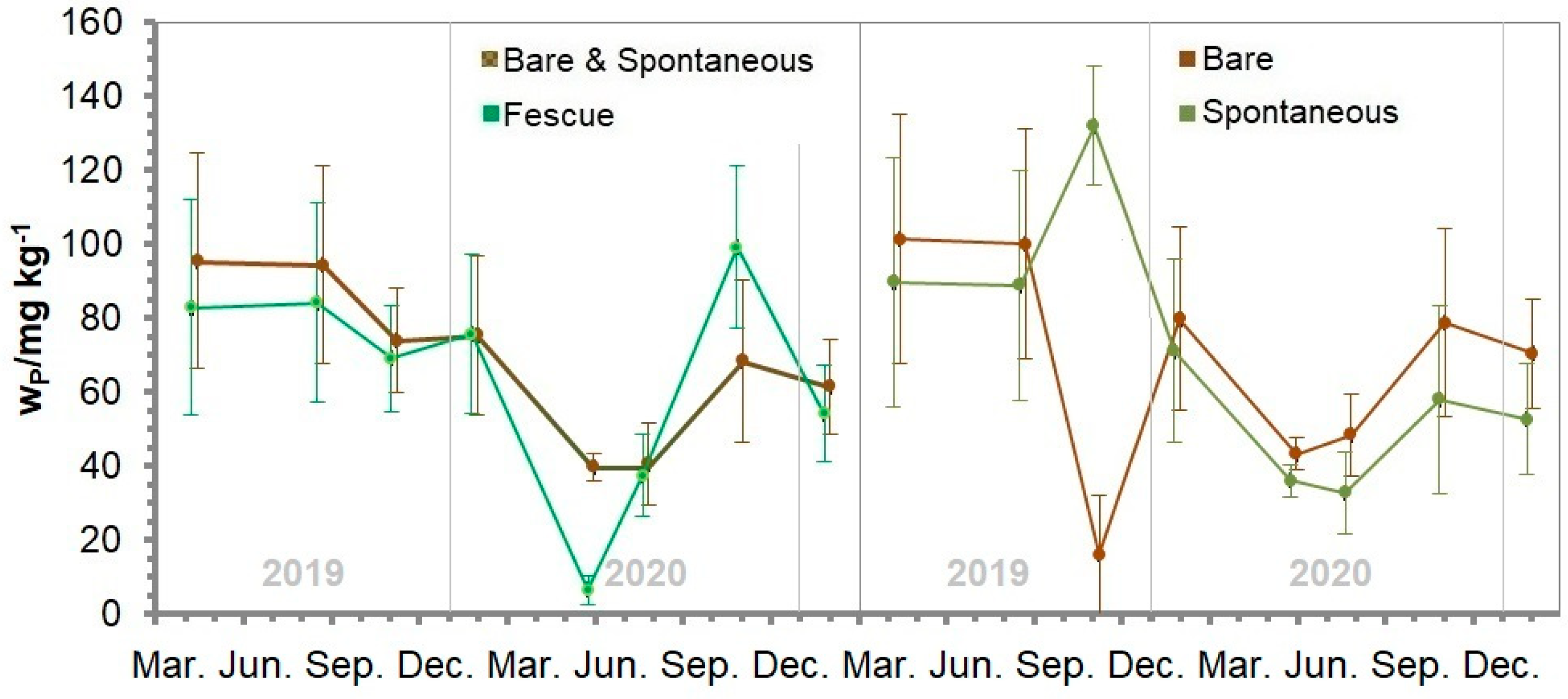
3.15. Soil Phosphorus

According to the two-way ANOVA (Table 3), there were highly significant differences among the different sampling times (p < 0.001) but not among the soil treatments (p = 0.47). However, since the magnitude or the direction of the treatments’ effects changed from one sampling to the other on the basis of the significant interaction (p < 0.001), eight one-way ANOVAs and eight batches of orthogonal contrasts were carried out to find if specific differences could be found. As a consequence, it was found that, in general, there were no differences between the combined bare and spontaneous treatments, on the one hand, and fescue, on the other, but that, interestingly, the spontaneous plants’ soil showed significantly lower available phosphorus than the bare soil in three out of the four last sampling times (Figure 11).

4. Discussion

4.1. Soil Characteristics

The soil in the study site has developed on a Middle Pleistocene marl runoff blanket [44,45]. Therefore, the soil in the study site is quite young, which is revealed by the fact that only an incipient decarbonation can be observed in the shallower 20 cm layer (Table 1). In addition, according to its bulk density, the topsoil was moderately compacted, featuring a pore space between 36 and 40% at the beginning of the monitoring. This compaction is a disturbance condition typically shared by most Valencian citrus plantations because of the agricultural vehicle traffic [12], leading to the low physical fertility of the inter-row soils.
The soil organic matter was also low according to the amount of clay and calcium carbonate equivalent following Rémy and Marin-Laflèche [46]. The optimum wSOC in the shallower 20 cm layer would be over 4.1%, according to these authors. Consequently, the soil in the study site shows damaged chemical fertility. However, it presents a potential carbon sequestration capacity of 1.5% of wSOC, which in case it was fulfilled, the wSOC would increase by 163%. Therefore, assuming a 4‰ annual rate of reasonable accumulation of SOM in agricultural soils following conservative practices [47], this increase of 163% may be achieved in 65 years.

4.2. Soil Fertility Drivers: Temperature and Water Content

Soil temperature and water content are the main drivers of soil fertility because they strongly regulate the vital functions of plants and soil organisms [48,49]. In this work, this was reflected by the significant correlations of T and θw with some biological activity indicators and nutrient contents (Table 2). Therefore, it is important to understand how the differences in the average daily topsoil temperature between the treatments depend on the magnitude of the energy inputs and outputs alongside the topsoil heat capacity. The topsoil temperature variation down to a depth of d can be assessed from (Appendix A):
Δ T = R s ( 1 α ) R lw h v E T S J H ( ρ b C s + ρ w θ w C w ) d
where the main warming-up (ΔT > 0) factor is the incident solar radiation (Rs). Conversely, the main cooling-down (ΔT < 0) factor is the reflected solar radiation, i.e., α Rs, the long-wave net radiation (Rlw), heat convection as latent heat, i.e., hv ET, sensible heat (S), and the heat conduction towards the subsoil (JH). In addition to these, there is the heat-buffering factor; this is the topsoil heat capacity in the denominator of Equation (8).
The soil temperature differences between the treatments may be understood, at least qualitatively, from Equation (8) by additionally considering that the average T values mostly reflected the maximum T values and not the minimum ones, which presented no variations between the treatments (Figure 2). The treatment that lowered the topsoil temperature the most was fescue. This is in accordance with Pradel and Pieri [50], who also observed lower soil temperatures under grass cover in comparison to plowing. Several processes may cause this T-lowering effect of fescue. First, there is the dimming of the warming-up factor, i.e., the solar radiation balance expressed by Rs (1 − α) in Eq. 8. Additionally, there is the increase in the cooling and heat-buffering factors, i.e., hv ET and ρb Cs + ρw θw Cw. Finally, there is the heat conduction factor (JH), as shown by Pradel and Pieri [50].
Which of these aforementioned effects dominate may be discovered by assessing their respective relative importance. Therefore, first, the soil’s surface albedo was estimated from its corresponding color value in the Munsell Color System [51] by using the relationship calibrated by Post et al. [52]. The soil surface color in the study site was visually estimated to be 7.5YR 5/5.5 in the Munsell Color System, thus giving an albedo of 23%, whereas grass covers present an albedo ranging between 20 and 27% [53], featuring an acceptable average of 23% [54]. Therefore, all three treatments can be regarded as having presented the same albedo, and, consequently, the albedo effect cannot explain why fescue decreased the topsoil temperature more than both the bare and spontaneous plants treatments. On the contrary, higher evaporation from the grass cover may explain the temperature decrease regarding the control due to the loss of latent heat through water transpiration, i.e., the hv ET. Note that the consequent decrease in the topsoil water content because of higher evapotranspiration in the fescue could decrease its heat capacity, thus fostering higher T, but also decrease its heat conduction, thus fostering lower T. Since soil T was not measured at different depths, these effects cannot be further disentangled. In the case of the spontaneous plants, the scarce covering of 10–20% during most of the year did not likely give rise to appreciable evapotranspiration differences in comparison to the bare treatment, and thus the T differences between the spontaneous and bare treatments did not consistently appear.
The average topsoil water content depends on the water inputs and outputs and, additionally, on its water holding capacity, which depends, in turn, on the texture and bulk density. Based on a simplified water balance down to a depth d, the following equation holds for assessing the topsoil water content (Δθw) differences between the inter-row soils subjected to different water inputs and outputs:
Δθw = RETP
where R is the rainfall infiltration, ET is the evapotranspiration, and P is the percolation to the underlying soil layers.
In accordance with this simplified water balance (Equation (9)), the main wetting factor (Δθw > 0) is R. Conversely, the main drying (Δθw < 0) factors are ET and P. Therefore, from Equation (8), the differences in the topsoil water content between the treatments can be explained, at least qualitatively.
Although fescue left the topsoil drier than the other treatments in summer, on average, fescue increased the water content by the most. However, fescue also featured a somewhat higher ρb and lower Ks than the other two treatments and, furthermore, it was the treatment with higher ET, in accordance with the lower temperature of the topsoil. Therefore, the topsoil under fescue lost more water by ET and did not develop the extra macroporosity that would have been needed to ease rainfall infiltration. Accordingly, the higher annual average, θw, cannot be credited to a lower water loss through ET and neither to a higher rainfall infiltration rate. On the contrary, the higher annual average, θw, may be attributed (i) to a lower loss of water through percolation and (ii) to an overall higher amount of infiltrated water. In the first case, a lower Ks in the topsoil can not only slow down rainfall infiltration but also water percolation to the underlying soil layers, thus increasing the annual average, θw, whether the second overcomes the first. In the second case, it can be hypothesized that the grass increased the effective rainfall by shielding the fallen water from solar radiation and wind. This way, the evaporation rate of the soil water slowed down; it had more time left to infiltrate into the soil, and the effect of the infiltration rate (Ks) lost relevance.
Interestingly, under the spontaneous plants, the soil presented somewhat lower ρb and higher Ks. It seems that this treatment increased macroporosity sufficiently to rise Ks. The microporosity increases under spontaneous plants in comparison to the seeded one, which was likely a consequence of the different ecology of one plant compared to the other, as is discussed next.

4.3. Soil Organic Carbon

No organic materials were intentionally incorporated into the soil in any treatment because tillage was completely avoided in all three. Therefore, the most important contribution to enhancing the SOC in all treatments was the rhizodeposition from the plants’ roots. Regarding this, fescue was the treatment that featured the highest topsoil root mass fraction. Then, the spontaneous treatment presented the second-most root mass fraction. However, under the spontaneous plants, the topsoil root mass fraction was not high enough to stand out significantly over the bare treatment. Even more interestingly, regardless of the magnitude and differences in the root mass fraction among the treatments, no differences in SOC were consistently found between them. Notwithstanding, differences in SOC increase during the monitoring time were found. Specifically, under the spontaneous plants, SOC increased the highest from the first until the last sampling (+47%), whereas the other two treatments led to lower increases: fescue (+30%) and bare (+17%) (Figure 8).
The higher root mass fraction under fescue supports the likely higher ET under this treatment, as the low average annual T and low summer θw suggested (Figure 3). The higher root mass fraction under fescue is, moreover, able to explain the lower topsoil exchangeable potassium that was observed under this treatment, which was absorbed by the fescue. Interestingly, the contrary was noticed under the spontaneous plants, which, somewhat surprisingly, were able to maintain exchangeable potassium not only higher than the fescue but also higher than the bare treatment. This significantly high exchangeable potassium under spontaneous plants regarding the bare soil may be caused by the ability of these native plants to foster an indigenous K-solubilizing microorganism community [55], which may have weathered the soil hydrated micas (illites) and feldspars and thus have mobilized some K+ ions from the crystal lattices of these major minerals in the soils of the Valencian province. Then, the high soil exchangeable potassium under the spontaneous plants regarding the fescue reflects that this grass, perhaps due to its allochthonous nature, does not foster an indigenous K-solubilizing microorganisms in the same way as spontaneous plants do. A similar effect was observed in the inter-rows of a coffee plantation where exchangeable potassium, magnesium, and calcium increased in the topsoil more below the spontaneous plants than below a cover crop [56]. Therefore, spontaneous plants, due to their own unforced nature, adapt better to the harsh environmental conditions in the inter-rows. The good adaptation of false barley to the high year-to-year rainfall variability in semi-arid Mediterranean areas has already been shown [57], and this adaptation ability may also appear in the soil exchangeable potassium, as is further discussed next.
Under the Mediterranean climate conditions of the study site, spring is rainy, and summer is dry (Figure 3). Therefore, during early to mid-spring, both fescue and spontaneous plants grow and absorb potassium from the soil. Then, as spring passes by and summer comes, fescue dries but a relevant part of its material does not decay, and hence some potassium is preserved in its dry tissues, and, as a consequence, it does not return to the soil. Contrary to this, the spontaneous plants dry, and their tissues extensively decay, thus returning the potassium they absorbed in early spring to the soil. This fits the pronounced soil cover change from spring to summer of 50–90% to 10–20% under spontaneous plants, which is mainly led by the false barley life cycle. Conversely, the magnitude of the cover change for fescue fluctuated much less, specifically from 80% to 60% at most. Note that the almost significantly higher soil CO2 emission rate under the spontaneous plants fits the higher decaying activity under this treatment, which stands up over the bare soil and, particularly, over the fescue. The faster decomposition rate of spontaneous ground covers in comparison to seeded ones has also been found in coffee plantations [58]. Furthermore, the specific difference in the soil CO2 emissions between the spontaneous plants and fescue in the present study, indicates that under the spontaneous plants, the CO2 emissions came more from heterotrophic than from autotrophic respiration. In this regard, note that the contribution from the autotrophic respiration under the spontaneous plants must be much less than under fescue on average during the season, as the remarkable differences in ground-cover changes along the year suggest.
Regarding the other major nutrients, the exchangeable potassium differences among the treatments were not replicated either by phosphorus or nitrogen. In the phosphorus case, no differences between the treatments were clearly observed. This may be because the K-solubilizing microorganism community is not able to weather the soil P minerals, e.g., apatite, as much as the K minerals or either the P-Olsen extractant is not able to reveal the differences in the available soil P among treatments [59]. In the nitrogen case, the differences between the treatments were not observed. Nitrogen was not provided in the form of either mineral or organic fertilizers to the inter-rows, and neither by symbiotic-living bacteria, since legumes were absent. Therefore, the only way nitrogen could have reached the soil under these conditions would have been through aerial wet or dry deposition and also by means of free-living nitrogen-fixing microorganisms. Both processes seem to have been hardly relevant in the study site, and, more interestingly, if present, they affected all the treatments to the same extent. Additionally, the average C/N ratio in the inter-row soils presented values between 6 and 11 along the season, with the spontaneous plants presenting the highest of these in early spring and the lowest in mid-summer. A C/N ratio of 6 is very low and typical of the last stages of soil organic matter evolution. The rapid transition from 11 to 6 under the spontaneous plants’ cover further supports the high rate of SOM mineralization under these conditions. Evidence indicates that for SOC build-up, nitrogen must be provided to the soil system, either through N-fixing organisms or by N-fertilizers [60,61,62,63], and that the absence of nitrogen supply to the soil eventually leads to SOC loss and land degradation [64,65]. Therefore, the absence of any nitrogen supply to the inter-row soil under both herbaceous covers can explain why these consistently exhibited the same SOC as the bare soil.
In the study site, the development of spontaneous plants triggered higher biological activity than the other treatments. This was reflected by the dehydrogenase activity, which was comparable to under fescue (Figure 5), by the CO2 emission, which was the highest (Figure 7), and by the C/N ratio, which changed the fastest in addition to attaining the lowest eventual value (Figure 10), but not by the β-D-glucosidase activity (Figure 6). This higher biological activity certainly included some soil macrofauna blooming, which fed on the plant debris and drilled burrows into the soil, which can explain the comparatively higher hydraulic conductivity and the lower bulk density of the spontaneous plants’ soil regarding the other two. The boost in the soil macrofauna populations, particularly earthworms, and the subsequent increase in macroporosity is commonplace in the transition to no-tillage, as reviewed by Kay and VandenBygaart [66]. Although the spontaneous ground cover had positive effects on the physical fertility, this amelioration was barely reflected in the SOC build-up, likely because of the scarce nitrogen. According to Novara et al. [67], at least five years are needed in this kind of Mediterranean citrus orchards for changes in SOC to appear. When soil nutrients are scarce, however, they may be delayed longer or not take place at all.
Although the inter-row soil in the study site was very physically degraded at the onset of the treatments and, moreover, the time throughout, to which the herbaceous covers were applied, is not too long, some practical recommendations can be already drawn. First, the positive behavior of the spontaneous ground cover regarding the seeded one in the study site makes the former the recommendable choice. Second, the soil management of the spontaneous cover should go beyond the mere “let it grow and cut from time to time” in order to enhance the inter-row SOC. It may be the annual winter application of N-rich amendments on the surface with minimum to no-tillage or, better, the fostering of N-fixing soil organisms. The effects of these recommendations should be investigated.

5. Conclusions

The changes in the topsoil energy and water balances, and not less importantly, the ecological characteristics of the seeded and spontaneous plants, affected the physical, chemical, and biological soil fertility in the inter-rows of the citrus orchard featured in this investigation. The fescue ground cover boosted biological activity, but no improvements were reflected by the physical fertility, which was kept essentially equal to the bare soil treatment. Conversely, though the spontaneous plants’ effects on the topsoil temperature and water content were scarcely distinguishable from the bare soil and, moreover, they contributed fewer rhizodepositions than fescue, they also increased the enzymatic activities and, additionally ameliorated the chemical fertility, particularly the exchangeable potassium. In addition, they enhanced physical fertility. Regarding this, presumably, the burrows drilled by the development of a macrofauna community, which effectively fed on the spontaneous plants’ debris, acted as vectors. The topsoil organic carbon slightly increased in all of the grass ground covers during the two-year monitoring, but no significant changes among the treatments were found overall. This may be due to the scarce soil nitrogen content, which is likely constraining primary productivity in the inter-rows, hence limiting topsoil organic carbon increase. In this citrus orchard, the seeded ground cover does not seem to contribute any benefit, rather the opposite, over the spontaneous plants. To enhance the effects of the spontaneous ground cover, an annual surface application of organic nitrogen-rich materials or the fostering of soil N-fixing organisms would be recommended alongside the “let it grow and cut from time to time” management method. More research is needed to know the possibilities for SOC enhancement of these recommendations.

Supplementary Materials

The following supporting information can be downloaded at: https://www.mdpi.com/article/10.3390/environments9120151/s1, Table S1: Statistical summary of the properties studied in this work.

Author Contributions

Conceptualization, F.V., C.B. and J.M.d.P.; methodology, F.V., C.B. and J.M.d.P.; software, F.V.; validation, F.V., E.P., C.B. and J.M.d.P.; formal analysis, F.V. and J.M.d.P.; investigation, F.V., E.P. and J.M.d.P.; resources, C.B. and J.M.d.P.; data curation, F.V., E.P. and J.M.d.P.; writing—original draft preparation, F.V.; writing—review and editing, F.V.; visualization, F.V.; supervision, F.V. and J.M.d.P.; project administration, J.M.d.P.; funding acquisition, J.M.d.P. All authors have read and agreed to the published version of the manuscript.

Funding

This research was funded by the European Rural Development Fund (EAFRD), grant numbers AG_COOP_A/2018/036 and AG_COOP_A/2021/015. The participation of Enrique Peiró was funded by the Operative Program of the European Social Fund of the Valencian Community 2014–2020 and the IVIA through a specialization scholarship.

Data Availability Statement

Data are available from the authors upon request.

Acknowledgments

We would like to thank Piedad Romero for her assistance with the laboratory analyses and field work, Alejandro del Castaño for his assistance with the field work and Inmaculada Nájera for her assistance with the project administration.

Conflicts of Interest

The authors declare no conflict of interest. The funders had no role in the design of the study; in the collection, analyses, or interpretation of data; in the writing of the manuscript; or in the decision to publish the results.

Appendix A

On the basis of the classical soil energy balance equation [68], the following equation for assessing the soil energy differences (ΔH) leading to temperature changes throughout one time span can be suggested:
ΔH = Rs (1 − α) − Rlwhv ETSJH
where Rs is the incident solar radiation, both direct and diffuse short-wave, α is the surface albedo, Rlw is the net soil long-wave radiation, hv is the latent heat of water evaporation, ET is the evapotranspiration, S is the combined heat conduction and convection to the atmosphere as a sensible heat, and JH is the heat transfer to the underlying soil layers. Second, the soil heat capacity is provided by Jury and Horton [68] as follows:
C = ρb Cs + ρw θw Cw
where θw is the soil water content, ρw the water density, and Cs and Cw are the heat capacities of, respectively, the soil solids and water. Then, by combining both equations, the soil temperature variation down to a depth of d can be assessed as follows:
Δ T = Δ H C d = R s ( 1 α ) R lw h v E T S J H ( ρ b C s + ρ w θ w C w ) d

References

  1. Abbott, L.K.; Murphy, D.V. Soil Biological Fertility: A Key to Sustainable Land Use in Agriculture; Springer: Dordrecht, The Netherlands, 2007; pp. 1–264. [Google Scholar]
  2. Pompilica, I.; Romulus, I. Sustainable development of agriculture as means of slowing down the exploitation of nonrenewable natural resources. In Proceedings of the 13th International Multidisciplinary Scientific Geo Conference: Surveying Geology and Mining Ecology Management, SGEM, Albena, Bulgaria, 16–22 June 2013; pp. 685–692. [Google Scholar]
  3. Melero, S.; Panettieri, M.; Madejón, E.; Macpherson, H.G.; Moreno, F.; Murillo, J.M. Implementation of chiselling and mouldboard ploughing in soil after 8 years of no-till management in SW, Spain: Effect on soil quality. Soil Tillage Res. 2011, 112, 107–113. [Google Scholar] [CrossRef]
  4. Pagano, M.C.; Dhar, P.P. Arbuscular mycorrhizal fungi under monoculture farming: A review. In Monoculture Farming: Global. Practices, Ecological Impact and Benefits/Drawbacks; Nath, T.K., O’Reilly, P., Eds.; Nova Science Publishers: New York, NY, USA, 2016; pp. 161–170. [Google Scholar]
  5. Le Gall, M.; Evrard, O.; Dapoigny, A.; Tiecher, T.; Zafar, M.; Minella, J.P.G.; Laceby, J.P.; Ayrault, S. Tracing sediment sources in a subtropical agricultural catchment of southern Brazil cultivated with conventional and conservation farming practices. Land Degrad. Dev. 2017, 28, 1426–1436. [Google Scholar] [CrossRef]
  6. Xu, Q.; Ling, N.; Chen, H.; Duan, Y.; Wang, S.; Shen, Q.; Vandenkoornhuyse, P. Long-term chemical-only fertilization induces a diversity decline and deep selection on the soil bacteria. mSystems 2020, 5, e00337-20. [Google Scholar] [CrossRef] [PubMed]
  7. dos Santos, C.V.; Levien, R.; Schwarz, S.F.; Mazurana, M.; Petry, H.B.; Zulpo, L.; Fink, J.A. Physical-hydraulic properties of a sandy loam typic paleudalf soil under organic cultivation of ‘montenegrina’ mandarin (Citrus deliciosa tenore). Rev. Bras. Cienc. Solo. 2014, 38, 1882–1889. [Google Scholar] [CrossRef] [Green Version]
  8. MAPA. Encuesta Sobre Superficies y Rendimientos de Cultivos. Resultados 2020; Ministerio de Agricultura, Pesca y Alimentación: Madrid, Spain, 2021; pp. 1–180.
  9. MAPA. Encuesta de Utilización de Productos Fitosanitarios Campaña 2019. Resultados Agosto 2021; Ministerio de Agricultura, Pesca y Alimentación: Madrid, Spain, 2021; pp. 1–56.
  10. Hondebrink, M.A.; Cammeraat, L.H.; Cerdà, A. The impact of agricultural management on selected soil properties in citrus orchards in Eastern Spain: A comparison between conventional and organic citrus orchards with drip and flood irrigation. Sci. Total Environ. 2017, 581, 153–160. [Google Scholar] [CrossRef] [Green Version]
  11. Morugán-Coronado, A.; García-Orenes, F.; Cerdà, A. Changes in soil microbial activity and physicochemical properties in agricultural soils in eastern Spain. Spanish J. Soil Sci. 2015, 5, 201–213. [Google Scholar] [CrossRef]
  12. Cerdà, A.; Novara, A.; Moradi, E. Long-term non-sustainable soil erosion rates and soil compaction in drip-irrigated citrus plantation in Eastern Iberian Peninsula. Sci. Total Environ. 2021, 787, 147549. [Google Scholar]
  13. Di Prima, S.; Rodrigo-Comino, J.; Novara, A.; Iovino, M.; Pirastru, M.; Keesstra, S.; Cerdà, A. Soil Physical Quality of Citrus Orchards Under Tillage, Herbicide, and Organic Managements. Pedosphere 2018, 28, 463–477. [Google Scholar] [CrossRef] [Green Version]
  14. Niu, Y.H.; Wang, L.; Wan, X.G.; Peng, Q.Z.; Huang, Q.; Shi, Z.H. A systematic review of soil erosion in citrus orchards worldwide. Catena 2021, 206, 105558. [Google Scholar]
  15. Adams, W.A. The effect of organic matter on the bulk and true densities of some uncultivated podzolic soils. J. Soil Sci. 1973, 24, 10–17. [Google Scholar] [CrossRef]
  16. Gosselink, J.G.; Hatton, R.; Hopkinson, C.S. Relationship of organic carbon and mineral content to bulk density in Louisiana marsh soils. Soil Sci. 1984, 137, 177–180. [Google Scholar] [CrossRef]
  17. Stavi, I.; Ungar, E.D.; Lavee, H.; Sarah, P. Grazing-induced spatial variability of soil bulk density and content of moisture, organic carbon and calcium carbonate in a semi-arid rangeland. Catena 2008, 75, 288–296. [Google Scholar] [CrossRef]
  18. Poeplau, C.; Don, A. Carbon sequestration in agricultural soils via cultivation of cover crops—A meta-analysis. Agric. Ecosyst. Environ. 2015, 200, 33–41. [Google Scholar] [CrossRef]
  19. Russell, J.S. Soil fertility changes in the long-term experimental plots at Klybybolite, South Australia I. Changes in pH, total nitrogen, organic carbon, and bulk density. Australian J. Agr. Res. 1960, 11, 902–926. [Google Scholar] [CrossRef]
  20. Blanco-Canqui, H.; Stone, L.R.; Schlegel, A.J.; Lyon, D.J.; Vigil, M.F.; Mikha, M.M.; Stahlman, P.W.; Rice, C.W. No-till induced increase in organic carbon reduces maximum bulk density of soils. Soil Sci. Soc. Am. J. 2009, 73, 1871–1879. [Google Scholar] [CrossRef]
  21. de Oliveira, F.E.R.; Oliveira, J.M.; Xavier, F.A.S. Changes in soil organic carbon fractions in response to cover crops in an orange orchard. Rev. Bras. Cienc. Solo. 2016, 40, e0150105. [Google Scholar] [CrossRef] [Green Version]
  22. Gu, C.; Liu, Y.; Mohamed, I.; Zhang, R.; Wang, X.; Nie, X.; Jiang, M.; Brooks, M.; Chen, F.; Li, Z. Dynamic changes of soil surface organic carbon under different mulching practices in citrus orchards on sloping land. PLoS ONE 2016, 11, e0168384. [Google Scholar] [CrossRef] [Green Version]
  23. Moreno, B.; García-Rodríguez, S.; Cañizares, R.; Castro, J.; Benítez, E. Rainfed olive farming in south-eastern Spain: Long-term effect of soil management on biological indicators of soil quality. Agric. Ecosyst. Environ. 2009, 131, 333–339. [Google Scholar] [CrossRef]
  24. Ramos, M.E.; Robles, A.B.; Sánchez-Navarro, A.; González-Rebollar, J.L. Soil responses to different management practices in rainfed orchards in semiarid environments. Soil Tillage Res. 2011, 112, 85–91. [Google Scholar] [CrossRef]
  25. Herencia, J.F. Enzymatic activities under different cover crop management in a Mediterranean olive orchard. Biol. Agric. Hortic. 2015, 31, 45–52. [Google Scholar] [CrossRef]
  26. Gavazzi, C.; Schulz, M.; Marocco, A.; Tabaglio, V. Sustainable weed control by allelochemicals from rye cover crops: From the greenhouse to field evidence. Allelopathy J. 2010, 25, 259–273. [Google Scholar]
  27. Blubaugh, C.K.; Hagler, J.R.; Machtley, S.A.; Kaplan, I. Cover crops increase foraging activity of omnivorous predators in seed patches and facilitate weed biological control. Agric. Ecosyst. Environ. 2016, 231, 264–270. [Google Scholar] [CrossRef] [Green Version]
  28. Tillman, G.; Schomberg, H.; Phatak, S.; Mullinix, B.; Lachnicht, S.; Timper, P.; Olson, D. Influence of cover crops on insect pests and predators in conservation tillage cotton. J. Econ. Entomol. 2004, 97, 1217–1232. [Google Scholar] [CrossRef]
  29. Koudahe, K.; Allen, S.C.; Djaman, K. Critical review of the impact of cover crops on soil properties. Int. Soil Water Conserv. Res. 2022, 10, 343–354. [Google Scholar] [CrossRef]
  30. Rubio-Asensio, J.S.; Hortelano, D.; Ramírez-Cuesta, J.M.; Parra, M.; Buesa, I.; Intrigliolo, D.S. How fertilization regime should be adapted when almond trees are grown under deficit irrigation and with cover crops? Insights and open questions from a field trial. Acta Hortic. 2022, 1333, 351–358. [Google Scholar] [CrossRef]
  31. Rodríguez-Ballesteros, C. Clasificación Climática de Köppen-Geiger (para España). Periodo de Referencia 1981–2010. Available online: https://climaenmapas.blogspot.com/p/pagina-koppen.html (accessed on 14 April 2021).
  32. Soil Survey Staff. Keys to Soil Taxonomy, 12th ed.; US Department of Agriculture—Natural Resources Conservation Service: Washington, DC, USA, 2014; pp. 1–372.
  33. Ingelmo, F.; Molina, M.J.; de Paz, J.M.; Visconti, F. Soil saturated hydraulic conductivity assessment from expert evaluation of field characteristics using an ordered logistic regression model. Soil Tillage Res. 2011, 115, 27–38. [Google Scholar] [CrossRef] [Green Version]
  34. Wu, L.; Pan, L.; Mitchell, J.; Sanden, B. Measuring saturated hydraulic conductivity using a generalized solution for single-ring infiltrometers. Soil Sci. Soc. Am. J. 1999, 63, 788–792. [Google Scholar] [CrossRef]
  35. Kutzbach, L.; Schneider, J.; Sachs, T.; Giebels, M.; Nykanen, H.; Shurpali, N.J.; Martikainen, P.J.; Alm, J.; Wilmking, M. CO2 flux determination by closed-chamber methods can be seriously biased by inappropriate application of linear regression. Biogeosciences 2007, 4, 1005–1025. [Google Scholar] [CrossRef]
  36. Livingston, G.P.; Hutchinson, G.L. Enclosure-based measurement of trace gas exchange: Applications and sources of error. In Biogenic Trace Gases: Measuring Emissions from Soil and Water; Matson, P.A., Harris, R.C., Eds.; Blackwell Science Ltd.: Oxford, UK, 1995; pp. 14–51. [Google Scholar]
  37. Casida, J.L.E.; Klein, D.A.; Santoro, T. Soil dehydrogenase activity. Soil Sci. 1964, 98, 371–376. [Google Scholar] [CrossRef]
  38. Tabatabai, M.A.; Bremner, J.M. Use of p-nitrophenyl phosphate for assay of soil phosphatase activity. Soil Biol. Biochem. 1969, 1, 301–307. [Google Scholar] [CrossRef]
  39. Bremner, J.M. 1996. Nitrogen total. In Methods of Soil Analysis. Part 3. Chemical Methods; Sparks, D.L., Page, A.L., Helmke, P.A., Loeppert, R.H., Soltanpour, P.N., Tabatabai, M.A., Johnston, C.T., Sumner, M.E., Eds.; SSSA, ASA: Madison, WI, USA, 1996; pp. 1085–1121. [Google Scholar]
  40. Walkley, A. A critical examination of a rapid method for determining organic carbon in soils: Effects of variation in digestion conditions and of inorganic soil constituents. Soil Sci. 1947, 63, 251–263. [Google Scholar] [CrossRef]
  41. Visconti, F.; Jiménez, M.G.; de Paz, J.M. How do the chemical characteristics of organic matter explain differences among its determinations in calcareous soils? Geoderma 2022, 406, 115454. [Google Scholar] [CrossRef]
  42. Kuo, S. Phosphorus. In Methods of Soil Analysis. Part 3. Chemical Methods; Sparks, D.L., Page, A.L., Helmke, P.A., Loeppert, R.H., Soltanpour, P.N., Tabatabai, M.A., Johnston, C.T., Sumner, M.E., Eds.; SSSA, ASA: Madison, WI, USA, 1996; pp. 869–919. [Google Scholar]
  43. Gee, G.W.; Or, D. Particle-size analysis. In Methods of Soil Analysis. Part 4. Physical Methods; Campbell, G., Horton, R., Jury, W.A., Nielsen, D.R., van Es, H.M., Wierenga, P.J., Dane, J.H., Topp, G.C., Eds.; SSSA, ASA: Madison, WI, USA, 2002; pp. 255–294. [Google Scholar]
  44. IGME. Mapa Geológico de España E. 1:50.000, Valencia (722); Instituto Geológico y Minero de España. Servicio de Publicaciones Ministerio de Industria: Madrid, España, 1972; p. 1. [Google Scholar]
  45. GVA. Mapa de Suelos de la Comunidad Valenciana. Valencia (722); Servei d’Estudis Agraris i Comunitaris: Valencia, España, 1996; pp. 1–101. [Google Scholar]
  46. Rémy, J.C.; Marin-Laflèche, A. L’analyse de la terre: Réalisation d’un programme d’interpretation automatique. Annales Agronomiques 1974, 25, 607–632. [Google Scholar]
  47. Minasny, B.; Malone, B.P.; McBratney, A.B.; Angers, D.A.; Arrouays, D.; Chambers, A.; Chaplot, V.; Chen, Z.-S.; Cheng, K.; Das, B.S.; et al. Soil carbon 4 per mille. Geoderma 2017, 292, 59–86. [Google Scholar] [CrossRef]
  48. Alvarez, G.; Shahzad, T.; Andanson, L.; Bahn, M.; Wallenstein, M.D.; Fontaine, S. Catalytic power of enzymes decreases with temperature: New insights for understanding soil C cycling and microbial ecology under warming. Global Chang. Biol. 2018, 24, 4238–4250. [Google Scholar] [CrossRef] [PubMed]
  49. Rasmussen, P.U.; Bennett, A.E.; Tack, A.J.M. The impact of elevated temperature and drought on the ecology and evolution of plant–soil microbe interactions. J. Ecol. 2020, 108, 337–352. [Google Scholar] [CrossRef]
  50. Pradel, E.; Pieri, P. Influence of a grass layer on vineyard soil temperature. Aust. J. Grape Wine Res. 2008, 6, 59–67. [Google Scholar] [CrossRef]
  51. Munsell Color. Munsell Soil Color Charts; Macbeth Division of Kollmorgen Instruments Corporation: New Windsor, NY, USA, 1994; p. 36. [Google Scholar]
  52. Post, D.F.; Fimbres, A.; Matthias, A.D.; Sano, E.E.; Accioly, L.; Batchily, A.K.; Ferreira, L.G. Predicting Soil Albedo from Soil Color and Spectral Reflectance Data. Soil Sci. Soc. Am. J. 2000, 64, 1027–1034. [Google Scholar] [CrossRef]
  53. Payero, J.O.; Neale, C.M.U.; Wright, J.L. Near-noon albedo values of alfalfa and tall fescue grass derived from multispectral data. Int. J. Remote Sens. 2006, 27, 569–586. [Google Scholar] [CrossRef]
  54. Allen, R.G.; Pereira, L.S.; Raes, D.; Smith, M. Crop Evapotranspiration: Guidelines for Computing Crop Water Requirements; FAO: Rome, Italy, 1998; pp. 1–300. [Google Scholar]
  55. Meena, V.S.; Maurya, B.R.; Verma, J.P. Does a rhizospheric microorganism enhance K+ availability in agricultural soils? Microbiol. Res. 2014, 169, 337–347. [Google Scholar] [CrossRef]
  56. Sarno, J.L.; Afandi, T.A.; Oki, Y.; Senge, M.; Watanabe, A. Effect of weed management in coffee plantation on soil chemical properties. Nutr. Cycling Agroecosyst. 2004, 69, 1–4. [Google Scholar]
  57. Johnston, M.B.; Olivares, A.E.; Calderón, C.E. Effect of quantity and distribution of rainfalls on Hordeum murinum L. Growth and development. Chil. J. Agric. Res. 2009, 69, 188–197. [Google Scholar] [CrossRef] [Green Version]
  58. Da Silva Matos, E.; Cardoso, I.M.; Souto, R.L.; De Lima, P.C.; De Sá Mendonça, E. Characteristics, residue decomposition, and carbon mineralization of leguminous and spontaneous plants in coffee systems. Commun. Soil Sci. Plant Anal. 2011, 42, 489–502. [Google Scholar] [CrossRef]
  59. Olego, M.Á.; Cuesta-Lasso, M.D.; Visconti Reluy, F.; López, R.; López-Losada, A.; Garzón-Jimeno, E. Laboratory extractions of soil phosphorus do not reflect the fact that liming increases rye phosphorus content and yield in an acidic soil. Plants 2022, 11, 2871. [Google Scholar] [CrossRef] [PubMed]
  60. Forrester, D.I.; Pares, A.; O’Hara, C.; Khanna, P.K.; Bauhus, J. Soil Organic Carbon is Increased in Mixed-Species Plantations of Eucalyptus and Nitrogen-Fixing Acacia. Ecosyst 2013, 16, 123–132. [Google Scholar] [CrossRef]
  61. Meng, F.; Dungait, J.A.J.; Xu, X.; Bol, R.; Zhang, X.; Wu, W. Coupled incorporation of maize (Zea mays L.) straw with nitrogen fertilizer increased soil organic carbon in Fluvic Cambisol. Geoderma 2017, 304, 19–27. [Google Scholar] [CrossRef]
  62. Sarma, B.; Gogoi, N. Nitrogen Management for Sustainable Soil Organic Carbon Increase in Inceptisols Under Wheat Cultivation. Commun. Soil Sci. Plant Anal. 2017, 48, 1428–1437. [Google Scholar] [CrossRef]
  63. Ball, K.R.; Baldock, J.A.; Penfold, C.; Power, S.A.; Woodin, S.J.; Smith, P.; Pendall, E. Soil organic carbon and nitrogen pools are increased by mixed grass and legume cover crops in vineyard agroecosystems: Detecting short-term management effects using infrared spectroscopy. Geoderma 2020, 379, 114619. [Google Scholar] [CrossRef]
  64. Raphael, J.P.A.; Calonego, J.C.; Milori, D.M.B.P.; Rosolem, C.A. Soil organic matter in crop rotations under no-till. Soil Tillage Res. 2016, 155, 45–53. [Google Scholar] [CrossRef] [Green Version]
  65. Rocha, K.F.; de Souza, M.; Almeida, D.S.; Chadwick, D.R.; Jones, D.L.; Mooney, S.J.; Rosolem, C.A. Cover crops affect the partial nitrogen balance in a maize-forage cropping system. Geoderma 2020, 360, 114000. [Google Scholar] [CrossRef]
  66. Kay, B.D.; VandenBygaart, A.J. Conservation tillage and depth stratification of porosity and soil organic matter. Soil Tillage Res. 2002, 66, 107–118. [Google Scholar] [CrossRef]
  67. Novara, A.; Pulido, M.; Rodrigo-Comino, J.; Prima, S.D.I.; Smith, P.; Gristina, L.; Giménez-Morera, A.; Terol, E.; Salesa, D.; Keesstra, S. Long-term organic farming on a citrus plantation results in soil organic carbon recovery. Geograph. Res. Lett. 2019, 45, 271–286. [Google Scholar] [CrossRef]
  68. Jury, W.A.; Horton, R. Soil Physics, 6th ed.; John Wiley and Sons: Hoboken, NJ, USA, 2004; pp. 1–370. [Google Scholar]
Figure 1. Location of the study site.
Environments 09 00151 g001
Figure 2. (a) Daily mean temperature at 5–10 cm depth in the different treatments; (b) daily maximum temperature; (c) daily minimum temperature.
Environments 09 00151 g002
Figure 3. Daily mean soil water content at 5–10 cm depth in the different treatments along with the cumulated rainfall during the monitoring time.
Environments 09 00151 g003
Figure 4. (a) Logarithm to base 10 of the soil surface saturated hydraulic conductivity (Ks) in the different treatments alongside the 95% confidence interval for the means according to the orthogonal contrasts based on the two-way ANOVA results; (b) bulk density (ρb) at 0–5 cm in the different treatments alongside the 95% confidence interval for the means according to the orthogonal contrasts based on the two-way ANOVA results.
Environments 09 00151 g004
Figure 5. (a) Square root of the soil root mass fraction (wroot1/2) at 0–5 cm in the different treatments alongside the 95% confidence interval for the means according to the orthogonal contrasts based on the two-way ANOVA results; (b) logarithm to base 10 of the dehydrogenase activity (DHA) at 0–20 cm in the different treatments alongside the 95% confidence interval for the means according to the orthogonal contrasts based on the two-way ANOVA results.
Environments 09 00151 g005
Figure 6. Logarithm to base 10 of the β-D-glucosidase activity (GLA) at 0–20 cm in the different treatments throughout five sampling dates during the monitoring time alongside the respective 95% confidence intervals according to the orthogonal contrasts based on the one-way ANOVAs results.
Environments 09 00151 g006
Figure 7. (a) logarithm to base 10 of the soil carbon dioxide emission (EC-CO2) in the different treatments alongside the 95% confidence interval for the means according to the orthogonal contrasts based on the two-way ANOVA results; (b) soil organic carbon mass fraction (wSOC) at 0–20 cm in the different treatments alongside the 95% confidence interval for the means according to the orthogonal contrasts based on the two-way ANOVA results.
Environments 09 00151 g007
Figure 8. Soil organic carbon mass fraction at 0–20 cm in the different treatments throughout all sampling dates during the monitoring time alongside the respective 95% confidence intervals according to the orthogonal contrasts based on the one-way ANOVAs results.
Environments 09 00151 g008
Figure 9. (a) logarithm to base 10 of the soil nitrogen mass fraction (wN) at 0–20 cm in the different treatments alongside the 95% confidence interval for the means according to the orthogonal contrasts based on the two-way ANOVA results; (b) logarithm to base 10 of the soil exchangeable potassium concentration (nK) at 0–20 cm in the different treatments alongside the 95% confidence interval for the means according to the orthogonal contrasts based on the two-way ANOVA results.
Environments 09 00151 g009
Figure 10. Soil carbon to nitrogen ratio, i.e., wSOC/wN (C/N), at 0–20 cm in the different treatments throughout the monitoring time alongside the 95% confidence interval for the means according to the orthogonal contrasts based on the one-way ANOVA results for each sampling time.
Environments 09 00151 g010
Figure 11. Soil available phosphorus (wP) at 0–20 cm in the different treatments throughout eight sampling dates during the monitoring time alongside the respective 95% confidence intervals according to the orthogonal contrasts based on the one-way ANOVAs results.
Environments 09 00151 g011
Table 1. Summary of the main soil characteristics 1 in the citrus orchard at the beginning of the study.
Depth/cmTexture USDAwSOM(%)wCCE(%)ρb/g cm−3
Clay (%)Silt (%)Sand (%)Class
0–20304229Clay loam1.4271.63
20–40264232Loam1.029
40–60294131Clay loam0.630
1 Depth: depth interval; wSOM: mass fraction of organic matter; wCCE: mass fraction of calcium carbonate equivalent; ρb: fine earth (<2 mm) bulk density.
Table 2. Pearson’s product-moment correlation coefficients among the soil variables 1 along with an indication of their significance at the 95% (*), 99% (**), and 99.9% (***) confidence level.
TθwLog
Ks
ρbwroot1/2Log DHALog GLALog EC-CO2wSOCLog wNLog
nK
θw−0.65 ***
Log
Ks
0.59−0.28
ρb0.010.25−0.77 **
wroot1/2−0.430.70−0.330.70
Log DHA0.50 ***−0.42 **0.020.090.38
Log GLA−0.040.23−0.25−0.310.820.04
Log_
EC-CO2
−0.110.36 *0.60−0.180.00−0.090.44 *
wSOC−0.030.120.190.020.200.270.18−0.15
Log wN0.67 ***−0.59 ***−0.250.36−0.84 *0.41 **0.18−0.260.21
Log
nK
−0.280.240.16−0.15−0.210.21−0.25−0.050.14−0.18
wP−0.06−0.11−0.00−0.090.65−0.07−0.18−0.16−0.07−0.17−0.08
1T: temperature; θw: water content; Ks: saturated hydraulic conductivity; ρb: fine earth (<2 mm) bulk density, wroot: soil root mass fraction; DHA: dehydrogenase activity; GLA: β-D-glucosidase activity; EC-CO2: carbon dioxide emission; wSOM: organic carbon mass fraction; wN: nitrogen mass fraction, nK: exchangeable potassium; wP: available phosphorus mass fraction.
Table 3. Two-way analyses of variance of the properties studied in this work 1, except for wroot1/2 for which the one-way ANOVA is shown.
PropertySource of
Variance
Degrees of FreedomSum of SquaresMean
Square
F-Valuep-Value
Log KsTreatment20.35530.17771.8690.1846
Measurement time10.55380.55385.8270.0273
Treat. × Meas.20.07310.03650.3840.6866
Residual171.61570.095
ρbTreatment20.008890.0044431.4610.2537
Sampling time20.028970.0144874.7630.0191
Treat. × Samp.40.014790.0036981.2160.3325
Residual220.066910.003042
wroot1/2Treatment22.307541.1537717.3030.000824
Sampling time
Treat. × Samp.
Residual90.60010.0667
Log DHATreatment20.2940.14723.1840.0453
Sampling time74.8120.687414.8651.85 × 10−13
Treat. × Samp.140.6210.04430.9590.4998
Residual1084.9950.0462
Log GLATreatment21.99930.999738.0273.96 × 10−12
Sampling time41.41320.353313.442.63 × 10−8
Treat. × Samp.80.84620.10584.0230.000512
Residual751.97160.0263
EC-CO2Treatment20.3560.17791.8220.166
Measurement time1511.2060.74717.6526.29 × 10−12
Treat. × Meas.303.6940.12311.2610.189
Residual12712.3990.0976
wSOCTreatment20.00560.002790.2660.767
Sampling time90.67580.075097.152.49 × 10−8
Treat. × Samp.180.20940.011631.1080.353
Residual1261.32320.0105
Log wNTreatment20.00240.00120.5120.601
Sampling time70.188090.0268711.4711.02 × 10−10
Treat. × Samp.140.050420.0036021.5380.111
Residual1040.243610.002342
Log nKTreatment20.22780.1139112.1780.0000177
Sampling time70.40010.057166.110.00000544
Treat. × Samp.140.18580.013271.4190.157
Residual1040.97280.00935
wPTreatment23701850.7630.469
Sampling time756819811733.497<2 × 10⁻¹⁶
Treat. × Samp.1449095350714.472<2 × 10⁻¹⁶
Residual10425201242
1T: temperature; θw: water content; Ks: saturated hydraulic conductivity; ρb: fine earth (<2 mm) bulk density, wroot: soil root mass fraction; DHA: dehydrogenase activity; GLA: β-D-glucosidase activity; EC-CO2: carbon dioxide emission; wSOM: organic carbon mass fraction; wN: nitrogen mass fraction, nK: exchangeable potassium; wP: available phosphorus mass fraction.
Publisher’s Note: MDPI stays neutral with regard to jurisdictional claims in published maps and institutional affiliations.

