Soil Loss Analysis of an Eastern Kentucky Watershed Utilizing the Universal Soil Loss Equation

Abstract

Soil erosion is the displacement of soil’s upper layer(s) triggered by a variation in topography, land use and soil types, and anthropogenic activities. This study selected the Marrowbone Creek-Russel Fork watershed in eastern Kentucky to estimate the mean annual soil loss over eight years (from 2013 to 2020) utilizing the Universal Soil Loss Equation (USLE). We included monthly precipitation, soil survey, digital elevation model (DEM), and land cover data to estimate the parameters of the USLE. The mean annual soil loss for the study area ranged from 1.77 to 2.91 Mg ha⁻¹ yr⁻¹ with an eight-year mean of 2.31 Mg ha⁻¹ yr⁻¹. In addition, we observed that developed land cover classes were less erosion-resistant than undeveloped land cover classes over the observation period. The results of this case study in our small watershed that has been historically impacted by upstream coal-mining activities are comparable to the results from similar studies in other geographic regions. However, we suggest other researchers conduct similar studies using robust data to determine the applicability of the USLE model and validate the results in developing measures to address soil loss issues.

1. Introduction

Soil erosion occurs when upper soil layer (s) are displaced in response to erosive agents [1]. Multiple factors accelerate this process such as topography, rainfall pattern/intensity, land use and land cover, and soil type. Globally, soil erosion is the cause for an estimated 75 petagrams (Pg = 10¹⁵ g) of fertile soil loss each year affecting negatively local agriculture, ecology, and climate [2]. While the negative consquencs of soil erosion is manifested in multiple ways, the removal of soil organic carbon (SOC) is the most notable. The organic matter existing in all the soils on the Earth contains approximately 2500 Pg of C (in the first 3 m depth), which is three times higher than the amount of C contained in the atmosphere and roughly 4.5 times the amount of C in the biosphere [3]. Since the Industrial Revolution, approximately 78 ± 12 Pg of C released into the atmosphere has directly resulted in depleting SOC, which is about 27–30% of the total global emission of C since the late 18th century [4]. Thus, research into the measuring and modeling of soil erosion is crucial to our understanding of the mechanics of how soil erosion compounds the effects of our changing climate and major implications for how well the outcomes can be modeled and predicted.

Water erosion (caused by the kinetic energy of raindrops and the resulting surface runoff from precipitation) contributes to the loss of nutrients in the soil (including organic matter) through three processes: sheet erosion, rill erosion, and gully erosion. Sheet erosion occurs when soil erodes in thin, uniform layers caused by the effect of rain and shallow surface flow [5]. Rill erosion occurs when sediment moves in response to flowing water from shallow drainage lines, known as “rills,” that are less than 30 cm deep. Gully erosion occurs when soil is removed in response to the formation of large drainage lines (30 cm or greater) from the concentration of smaller streams that cut a channel through the soil.

The Universal Soil Loss Equation (USLE) (Equation (1)) is a commonly used mathematical model to examine the soil erosion process [6]. It is an empirical model based on five contributing factors, namely rainfall (R), soil erodibility (K), land slope (LS), cover management, © and conservation support practices (P). The USLE is used to predict long-term average annual soil loss, and it is an indispensable tool for predicting and estimating soil loss from sheet and rill erosion.

The soil erosion rate at a given site is determined by the combined contributions of the physical and management variables present at the site [7]:

A = R × K × L.S. × C × P

(1)

where A is the annual soil loss (Mg ha⁻¹ yr⁻¹), R is the rainfall erosivity index (MJ mm ha⁻¹ h⁻¹ yr⁻¹), K is the soil erodibility factor (Mg ha h MJ⁻¹ mm⁻¹), L.S. is the slope and slope length factor, C is the cover management factor, and P is the support practice factor.

The rainfall erosivity factor (R) measures the amount of precipitation and the corresponding energy effects of precipitation on soil [8]. Runoff (water from rain, melting snow, or other sources that flow over land surfaces) is linearly related to rainfall through a ratio of the retention of water in a watershed during a storm event to the maximum potential retention of water in the watershed [9]. The following Equation (2) is used to determine the average annual R factor (MJ mm ha⁻¹ h⁻¹ yr⁻¹) [10]:

$$\mathrm{R}=\frac{1}{n}{\displaystyle \sum _{j=1}^n}{\left[{\displaystyle \sum _{k=1}^n}{(\mathrm{E})}_k{{(\mathrm{I}}_{30})}_k\right]}_j$$

(2)

where E is the total storm kinetic energy (MJ ha⁻¹), I₃₀ is the maximum 30 min rain rainfall intensity (mm h⁻¹), j is an index of the number of years used to produce the average, k is an index of the number of storms in each year, n is the number of years used to obtain the average R.

R factor estimates are necessary to implement the USLE within regions with limited precipitation historical records [11]. Early examples of R factor estimates would be the modified Fournier Index (F), which was developed in Morocco using R-factor values from 178 weather stations [12]. The modified Fournier Index is represented by the equation:

$$\mathrm{F}=\frac{{{\displaystyle \sum }}_{i=1}^{12}{p}_i^2}{\mathrm{P}}$$

(3)

where $p_i$ is the average monthly precipitation, and P is the average annual precipitation. Later developments led to the development of monthly precipitation-based methods for calculating the R from 155 weather stations between 1951–1980 [13,14,15,16]. From this research, the following regression equation was developed for determining the R-factor in the continental United States using the modified Fournier Index [11]:

$$\mathrm{R}=0.07397{\mathrm{F}}^{1.847}$$

(4)

In this equation, R is the rainfall erosivity factor (MJ mm ha⁻¹ h⁻¹ yr⁻¹) and F is the modified Fournier Index.

The soil erodibility factor (K) denotes the vulnerability of soil to erosion and its potential runoff rate [17]. It is based on several physical soil characteristics: sand content (in percentage), silt content (in percentage), clay content (in percentage), and soil organic matter (in percentage) [18]. Soils that are more resistant to erosion have low K factor values, while soils that are less resistant to erosion have higher K factor values. Soils with more clay content tend to be more resistant to soil erosion and have low K factor values, as they tend to be more resistant to detachment. Soils with more silt content tend to be more erosive and produce more runoff due to being more susceptible to detachment, and thus produce high K factor values.

In the U.S., K-factor-related soil data can be obtained through the Soil Survey Geographic Database (SSURGO) via the ‘USDA’s Natural Resources Conservation Service (NRCS) [19]. The K factor values from this database are derived from the following equation [18]:

$$A_u=E.I{.}_{30}K$$

(5)

where, $A_u$ is soil loss measured for individual storms, K is the soil erodibility value for each soil type, and $E.I{.}_{30}$ represents erosivity of the storms for the respective soil loss values (Equation (5)).

The topographic factor (L.S.) shows the effect of length of slope and slope steepness on soil erosion rate by water [7]. Slope Length (L) denotes the distance from the origin of overland flow to the point where either soil deposition starts, or the runoff becomes intense [20]. Slope Steepness (S) represents the effect of the uniform slope values on erosion. Consequently, the product (L.S.) represents the estimated ratio of soil loss per unit area from a field slope to that from a 9 percent slope that is 72.6-ft (approximately 22.13 m) long [6]. This ratio is calculated through the equation [20]:

$$\mathrm{L}.\mathrm{S}.=(\mathrm{A}/22.13)^(\mathrm{m}) \times (65.41{\sin }^2\theta +4.65\sin \theta +0.065)$$

(6)

where, A is the upslope factor (calculated from the flow accumulation tool),$\theta$ is the slope angle (calculated from the DEM) in radians, and m is a model parameter that equals 0.2 when the slope is less than 1%, 0.3 when the slope is between 1 and 3%, 0.4 when the slope is between 3 and 5%, and 0.5 when the slope is above 5%. For the purpose of GIS implementation, the modified equation for L.S. replaces slope length measurement with the measurement of the upslope contributing Area, A, which includes the effect of flow convergence from rill erosion [21].

Soil erosion grows as the slope rises and lengthens [22]. Longer slopes increase the soil transport and deposition capacities of a watershed by increasing the accumulation of runoff [7,23]. In a study of erosion hotspots within two central Ohio watersheds, the land slope was determined to have the most profound effect on erosion estimates within the watersheds [24].

The cover management factor (C factor) indicates the degree of soil erosion caused by different forms of land-uses [24]. The C factor shows the ratio of the expected soil loss from a cropped land under a particular condition to the equivalent loss of a similar field that was clean-tilled and fallow.

Numerous studies have found a correlation between NDVI (Normalized Difference Vegetation Index) and the C factor [25,26,27,28]. An advantage of NDVI-derived methods for computing the C factor is that it allows for more pixel-by-pixel variation in C factor values across the study area than traditional methods of assigning prescribed C factor values through classified satellite imagery [26]. This allows for the C factor to account for the spatio-temporal variation in crop management [28]. However, modeling sensitivity to this remote sensing method can cause an overestimation of C factor values, which yield higher annual mean soil loss rate values [29].

This study examines the effects of the various erosion factors on the USLE model output for the Marrowbone Creek-Russell Fork watershed in eastern Kentucky over an eight-year period (2013–2020) and determine if developed land (“built-up” land containing man-made structures) in the studied watershed is more erosion-resistant than the undeveloped land (forest land, grassland, and barren land) in our watershed [30]. The study focused on three objectives: (1) estimate the value of factors in the USLE from geospatial and meteorological data for this watershed; (2) evaluate the applicability of Landsat 8 NDVI to estimating factors in USLE; and (3) estimate the soil erosion rate for the area for the observation years (2013–2020) based on annual estimates of USLE factors and visual imagery interpretation.

2. Materials and Methods

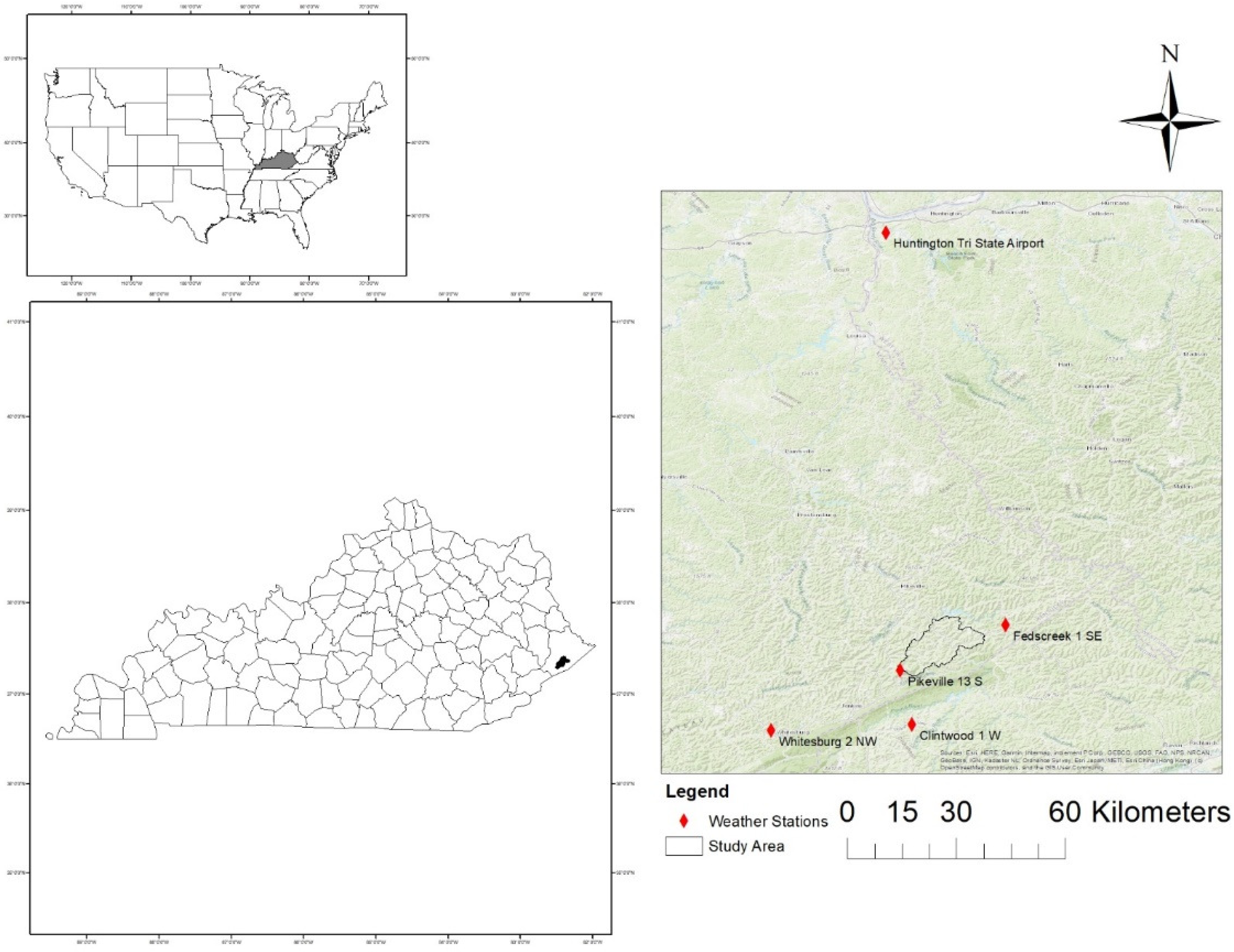
2.1. Study Area

The study site (latitude: 37.31, longitude: −82.42) is the Marrowbone Creek-Russell Fork watershed (Hydrological 12-digit Unit: 050702020704), located in Pike County, Kentucky [31]. The watershed has an area of 153.16 km² and elevations ranging from 203 to 863 m, with an average percent slope of 16.38%. Kentucky experiences a humid subtropical climate characterized by hot summers, cold winters, sunny autumns, and mild but wet springs. In Pike County (the county where our study site resides), the annual average temperature is approximately 13.11 °C. The annual average rainfall was recorded at approximately 1148 mm [32].

Our study site is in a region of eastern Kentucky, which experienced surface mining activity in the past in towns such as Regina (within the watershed) and Wolfpit (near the watershed). The watershed also consists of areas currently under coal-mining activity, such as the Clintwood Elkhorn Mining Company (approximately 9 km from the study site). That, along with the study ‘site’s internal land use being mainly undisturbed forestland with some developed land spaces and pasture, makes the study site ideal for estimating and analyzing soil erosion rates from mined eastern Kentucky watershed.

2.2. Universal Soil Loss Equation (USLE)

The USLE is fully described in Equation (1). We estimated the soil loss using USLE in ArcGIS Desktop (a part of the Esri suite of GIS software).

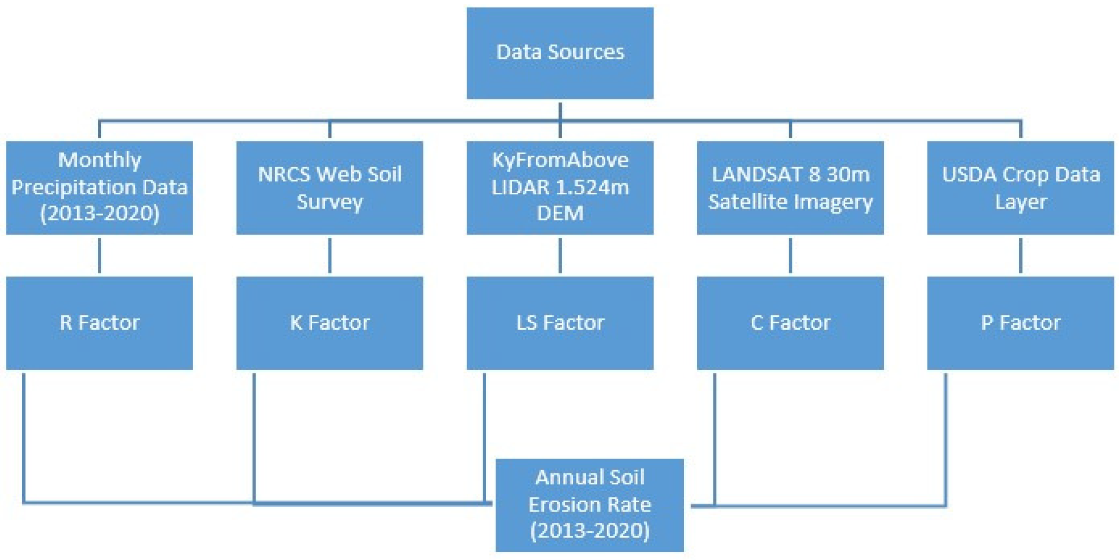
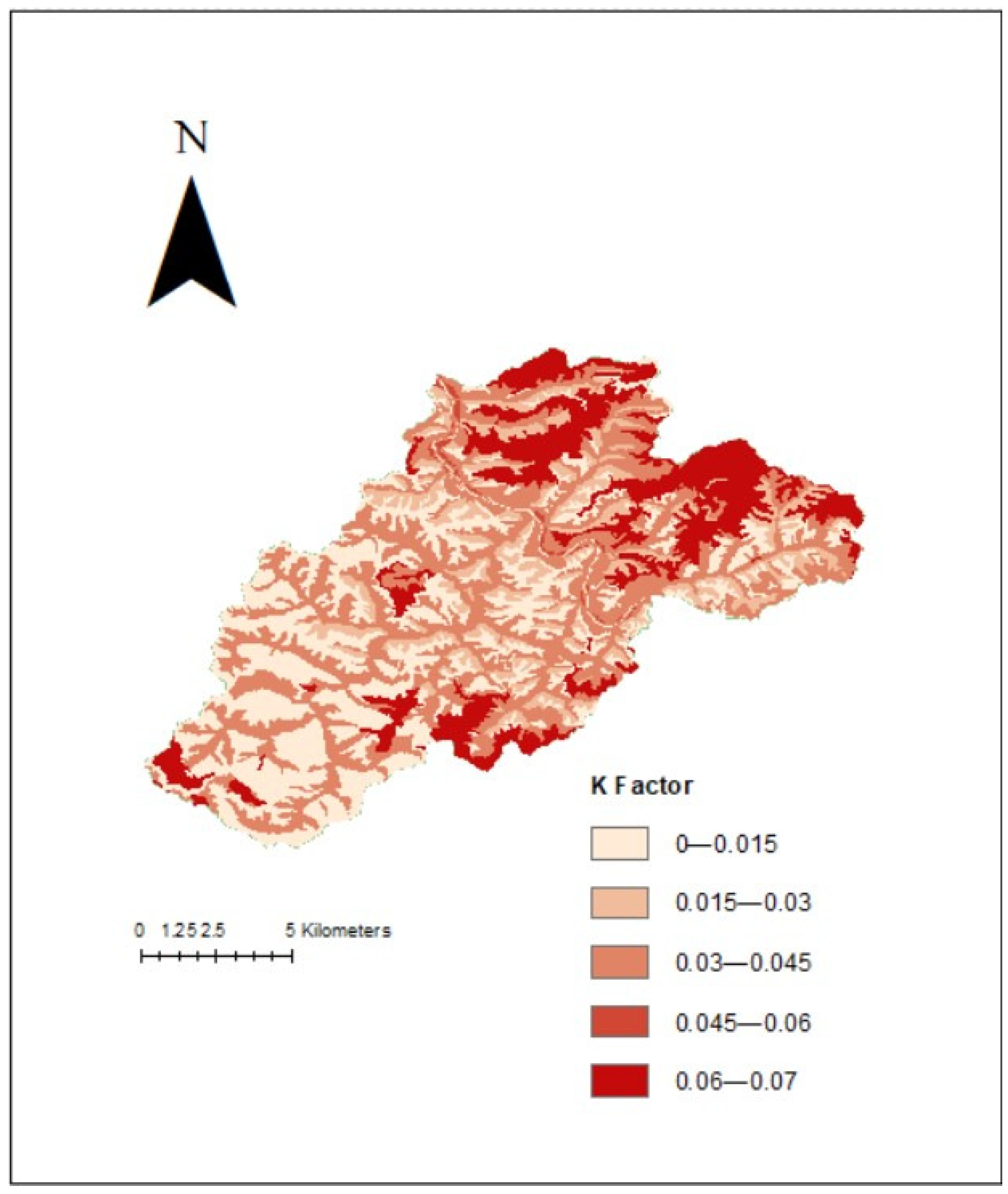
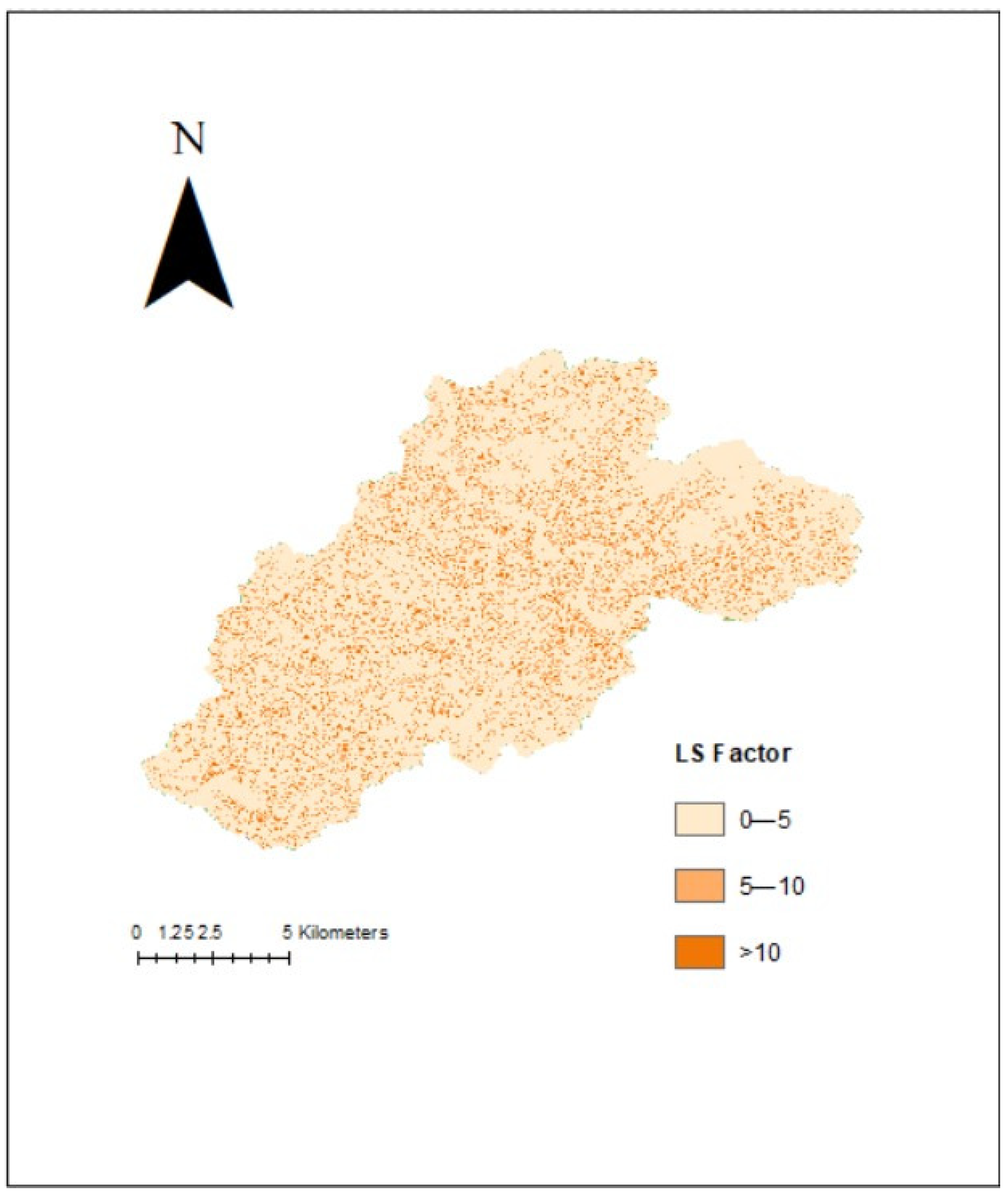
2.3. Data Collection and Processing

For our project, monthly precipitation data, soil survey data, terrain data, satellite imagery, and land cover classification data were collected for the eight-year period of our study (2013–2020) from several online data repositories. All data were converted to have the spatial resolution of 30 m.

To calculate rainfall/runoff erosivity index, we acquired monthly precipitation data from five weather stations that surround the watershed over a period of eight years (2013–2020) (Figure 1).

Table 1. List of weather stations that provided monthly precipitation data for the project.

Organization	City (Location)	Station ID	Latitude	Longitude
Kentucky Mesonet	Pikeville 13 S	DORT	37.28	−82.52
NCDC (NOAA)	Fedscreek 1 SE	USC00152812	37.39	−82.26
NCDC (NOAA)	Clintwood 1 W	USC00441825	37.15	−82.49
NCDC (NOAA)	Huntington Tri State Airport	USW00003860	38.37	−82.55
Kentucky Mesonet	Whitesburg 2 NW	WTBG	37.13	−82.84

provides additional information on the five weather stations from which we acquired the monthly precipitation data.

The data for the soil erodibility (K) factor was acquired from the United States Department of Agriculture, Natural Resources and Conservation Services (NRCS) online web soil survey [33]. The NRCS online web soil survey provides comprehensive soil reports for an area defined by an Esri Shapefile.

Topographic (LS) ‘factor’s data was derived from ‘KyFromAbove’s 2020 5ft (approximately 1.5 m) Digital Elevation Model (DEM). This DEM provides the highest spectral resolution currently available for our watershed.

We used Landsat 8 satellite imageries from April 2013 to December 2020 to compute the crop management factor (C) values. The satellite imageries were downloaded from the ‘USGS’s Earth Explorer hub [34]. The individual satellite scenes were divided by the date when they were initially captured by the satellite to represent the four seasons: spring (March–May), summer (June–August), fall (September–November), and winter (December–February). For each date, two spectral bands (Band 4 and Band 5) were collected, as they provide the values for visible (red) light and near-infrared light, respectively.

Finally, the data for our Support Conservation Practice Factor (P) was from the Crop Data Layer from the ‘USDA’s National Agricultural Statistics Service [35] between 2013 and 2020.

Table 2. List of Parameters for Universal Soil Loss Equation with their data sources.

Parameters	Definition	Source	Original Spatial Resolution	Date of Acquisition
R (MJ mm ha−1 h−1 yr−1)	Rainfall/Runoff Erosivity Index	5 Stations: 2 Kentucky Mesonet stations; 3 NOAA stations	N/A	15 March 2021
K (Mg h MJ−1 mm−1)	Soil Erosivity Factor	NRCS web soil survey	N/A	11 November 2020
LS	Slope and length of Slope Factor	KyFromAbove LIDAR DEM 5 ft (1.524 m)	1.524 m	24 March 2021
C	Cover Management Factor	Landsat 8 Data	30 m	19 June 2021
P	Supporting Conservation practices	USDA Crop Data Layer, USDA RUSLE Guide	30 m	14 April 2021

provides additional information on the various data sources for the model parameters.

For the rainfall/runoff erosivity, we generated a table in Excel utilizing monthly precipitation data collected from five weather stations (see Table 1). We then utilized our monthly precipitation data to compute the Modified Fournier Index (F) [12], with p being average monthly precipitation and P being the annual total precipitation (Equation (3)). We did this for each year from 2013–2020. Afterward, we calculated the rainfall erosivity index for each year, utilizing the regression equation proposed in Equation (4).

The K factor for the equation was generated after importing the soil survey data in ArcMap. The polygon data was generated from the NRCS web soil survey, which has soil data originating from the national Soil Survey Geographic Database (SSURGO). Finally, the data were converted into a raster, and the K factor values were converted from U.S. customary units into S.I. units (Mg h⁻¹ MJ⁻¹ mm⁻¹) [36].

We calculated the L.S. (Slope and Length of Slope factor) by importing elevation KYAPED (LiDAR) DEM data. The L.S. factor was calculated using the slope tool, flow direction tool, flow accumulation tool, and, finally, the raster calculator, all in ArcMap. The slope tool was used twice: firstly, to generate a slope (in degrees) map from the 1.5 m DEM map of the watershed; secondly, to generate a slope percentage map where the slopes calculated in our watershed were separated into four classes (slopes less than 1%, slopes between 1–3%, slopes between 3–5%, and slopes greater than 5%) [20]. The flow direction and flow accumulation tools were used to simulate the movement of eroded soil throughout the watershed. Then, the raster calculator computed the L.S. factor with the USLE-Forest (Equation (6)).

We estimated the C factor by utilizing the NDVI values derived from Landsat 8 for the watershed. NDVI measures the density of green leaf vegetation by computing the difference in the reflection of near-infrared wavelengths of sunlight and visible wavelengths of sunlight divided by the sum of both near-infrared and visible reflected light.

$$\mathrm{NDVI}=\frac{\mathrm{near} \mathrm{infrared} \mathrm{light} - \mathrm{visible} \mathrm{light}}{\mathrm{near}\text{-}\mathrm{infrared} \mathrm{light}+\mathrm{visible} \mathrm{light}}$$

(7)

We calculated the NDVI for each season (spring, summer, fall, winter) of every year during our eight-year period by taking each satellite scene and substituting their spectral band imagery (Band 5 for near-infrared light and Band 4 for visible light) into Equation (7). Afterwards, we used the Raster Calculator within ArcMap to average the four seasonal NDVI maps for every year of our study. Next, we applied the following equation for generating the C factor using the average yearly NDVI and produced each ‘year’s mean annual C factor [27]:

$$\mathrm{C}=0.1(\frac{-\mathrm{NDVI}+1}{2})$$

(8)

To account for our limited knowledge in the conservation support practices within our watershed (which is mainly comprised of undeveloped forestland that would have a P factor of 1 to indicate zero support practices being applied), we incorporate a method proposed by Naqvi et al. [17] that uses the average P factor values calculated for each land cover class (as shown in

Table 3. Land cover classes and their respective P factor values.

Land Cover Classes	P Factor Values
Dense Vegetation	1
Sparse Vegetation	0.8
Built-up (Developed)	1
Water Bodies	1
Scrub Land	1
Agricultural cropland	0.5
Fallow Land	0.9
Bare Soil/Barren Land	1

).

We calculated the P factor by importing land cover data from the USDA Crop Data Layer [35]. Then, we reclassified the different land classes to conform the land cover classes to fit the land cover classes utilized by the USDA in reference to each ‘class’s respective P factors. Finally, we utilized the USDA Handbook No. 537 [7] to appropriately assign the average P factor values to each land cover class.

3. Results

Descriptive Statistics

Descriptive statistics of mean, minimum, and maximum values for the yearly mean R factors, K factor, L.S. factor, the yearly mean C factors and the yearly mean soil loss estimates (A) for the watershed were calculated using Microsoft Excel 2016. In addition, the ‘Zonal Statistics as ‘Table’ tool in ArcMap was utilized to determine the mean soil loss estimates, K factor, L.S. factor, and mean C factor for each land cover class.

We found the yearly precipitation ranged from a minimum of 1203 mm in 2016 to a maximum of 1638 mm in 2018 (mean equals 1361 mm) (

Table 4. Estimated annual mean R factor values from 2013–2020.

Year	Yearly Precipitation (mm)	MFI (mm)	R Factor (MJ mm ha−1 h−1 yr−1)
2013	1375.4	137.9	661.9
2014	1209.4	114.7	471.7
2015	1331.3	134.8	635.0
2016	1203.0	127.5	573.0
2017	1317.9	138.1	667.6
2018	1638.0	150.1	775.1
2019	1364.2	137.3	657.7
2020	1452.2	137.3	658.1

). The Modified Fournier Index (MFI) ranged from a minimum of 115 mm in 2014 to a maximum of 150 mm in 2018 (mean equals 136 mm). The annual R factors ranged from a minimum of 472 MJ mm⁻¹ ha⁻¹ h⁻¹ yr⁻¹ in 2014 to a maximum of 775 MJ mm ha⁻¹ h⁻¹ yr⁻¹ in 2018 (mean = 638 MJ mm ha⁻¹ h⁻¹ yr⁻¹).

The resultant K factor map is (Figure 2) based on the NRCS soil report data that was imported into ArcMap and converted into a raster format. The estimated K factor values ranged from 0 to 0.6 (Mg h⁻¹ MJ⁻¹ mm⁻¹), with a mean K factor value equal to 0.031 (Mg h ⁻¹ MJ⁻¹ mm⁻¹). Figure 3 and Figure 4 shows the raster map generated from the estimated L.S. factor values within our watershed. The raster had minimum estimated values of zero, a maximum estimated value of 15,815, and a mean estimated value of 3.6.

Computed yearly C factor for the eight years of our study is presented in

Table 5. Estimated annual mean C factor values from 2013–2020.

Year	NDVI	C Factor
2013	0.244	0.038
2014	0.215	0.039
2015	0.256	0.037
2016	0.225	0.038
2017	0.311	0.034
2018	0.227	0.039
2019	0.299	0.035
2020	0.269	0.037

. The C factors ranged from a minimum of 0.034 in (change to SI units) 2017 to a maximum of 0.039 in (ditto) 2014 (mean = 0.037). The NDVI values ranged from a minimum of 0.215 in 2014 to a maximum of 0.311 in 2017 (mean = 0.256). In

Table 6. Land cover classes with P factor and Area percentage of watershed.

		% of Watershed
Land Cover Classes	P Factor	Average % of Watershed	Area of Watershed (sq. km)	2013	2014	2015	2016	2017	2018	2019	2020
Corn	0.5	0	0	0	0	0	0	0	0	0	0
Other Hay/Non Alfalfa	0.9	0	0	0	0	0	0	0	0	0	0
Open Water	1	0.2	0.4	0.3	0.2	0.2	0.2	0.2	0.2	0.2	0.2
Developed/Open Space	1	2.3	3.5	3.0	2.2	2.1	2.1	2.1	2.1	2.4	2.4
Developed/Low Intensity	1	1.8	2.7	1.4	1.9	1.9	1.9	1.9	2.0	1.5	1.5
Developed/Med intensity	1	0.7	1.1	0.4	0.7	0.8	0.8	0.9	0.7	0.7	0.7
Developed/High Intensity	1	0.1	0.1	0.1	0.1	0.1	0.1	0.1	0.1	0.1	0.1
Barren	1	3.2	4.9	1.2	2.3	4.5	3.1	4.6	3.3	3.6	3.2
Deciduous Forest	1	78.7	120.6	71.3	70.2	79.5	79.9	79.6	78.7	85.1	85.3
Evergreen Forest	1	0.1	0.2	0	0	0	0	0	0	0.3	0.5
Mixed Forest	1	0.5	0.8	0.8	0.1	0.2	0.4	0.2	0.7	0.9	0.9
Shrubland	1	0.8	1.2	0	0	0	0.1	0.1	0.1	2.9	2.8
Grassland/Pasture	0.9	11.6	17.8	21.6	22.2	10.7	11.4	10.4	12.1	2.2	2.3
Woody Wetlands	0.8	0	0	0	0	0	0	0	0	0	0
Soybeans	0.5	0	0	0	0	0	0	0	0	0	0
Herbaceous Wetlands	0.8	0	0	0	0	0	0	0	0	0	0

, we presented the 16 land cover classes found in the watershed, along with their respective P factors, the estimated average percentage of areas they cover within the watershed, and the estimated percentage of Area they covered within the watershed each year from 2013–2020.

Our second objective was to calculate the mean C factor for three types of land use: (urban, forest, and grassland) (

Table 7. Mean C Factor and area percentage of watershed per land use.

Land Use	% of Watershed	Mean C Factor
Urban	4.9	0.039
Forest	79.3	0.037
Grassland	11.6	0.037

). The urban land use group included the average C over eight years based on land cover type, i.e., developed/open space, developed/low intensity, developed/medium intensity, developed/high intensity. The urban land use group covered 4.9% of the watershed with a mean C of 0.039.

The Forest land use group comprises the average C over eight years for the land cover types: deciduous forest, evergreen forest, and mixed forest. The forest land use group covered 79.3% of the watershed and with a mean C value of 0.038.

The grassland land use group included the average C over eight years for the grassland/pasture land cover type. The grassland land use group covered 11.6% of the watershed and with a mean C value of 0.037.

Our third objective was to calculate the mean annual estimates of soil loss (in Mg ha⁻¹ yr⁻¹) for the eight-year period (

Table 8. Annual Soil Erosion Estimates from 2013–2020.

		Rate of Soil Loss (Mg ha−1 yr−1)
Year	Mean Annual Soil Loss Estimate (A)	Low (A < 1.5)	Moderate (1.5 < A < 5)	High (A > 5)
2013	2.4	63.4%	25.4%	11.2%
2014	1.8	70.2%	23.0%	6.8%
2015	2.3	64.5%	25.2%	10.3%
2016	2.2	65.7%	24.6%	9.7%
2017	2.2	65.5%	25.0%	9.5%
2018	2.9	59.4%	26.2%	14.4%
2019	2.3	64.7%	24.8%	10.5%
2020	2.4	64.1%	25.4%	10.5%

) and the annual rate of soil loss based on the percentage of three soil erosion classes (low, moderate, and high). The lowest annual mean estimate occurred in 2014, with an estimated mean of 1.8 Mg ha⁻¹ for soil lost through erosion. The highest annual mean estimate occurred in 2018 when an estimated 2.9 Mg ha⁻¹ of soil was lost through erosion. The average mean soil loss estimate for the eight-year period was 2.3 Mg ha⁻¹ yr⁻¹. We used the mean annual soil loss estimates for each land cover type (

Table 9. Estimates of 8-year mean annual values of USLE parameters for each land cover class.

Land Cover Class	A	K	LS	C	P
Open Water	3.8	0.019	7.5	0.041	1.0
Developed/Open Space	3.4	0.032	4.4	0.038	1.0
Developed/Low Intensity	3.8	0.037	4.1	0.039	1.0
Developed/Med intensity	2.5	0.041	2.4	0.040	1.0
Developed/High Intensity	1.0	0.045	0.9	0.042	1.0
Barren	2.5	0.056	1.8	0.039	1.0
Deciduous Forest	2.5	0.027	3.8	0.037	1.0
Evergreen Forest	2.2	0.034	2.6	0.039	1.0
Mixed Forest	8.2	0.028	11.8	0.039	1.0
Shrubland	1.4	0.050	1.2	0.037	1.0
Grassland/Pasture	2.2	0.050	2.1	0.037	0.9

) to estimate the mean annual soil loss of developed land versus undeveloped land (

Table 10. Area Percentage and estimated area-weighted mean soil loss rate of Developed Land and Undeveloped Land.

Land Cover Type	Mean % of Watershed Area	Estimated Mean Soil Loss Rate (Mg ha−1 yr−1)
Developed Land	4.9	3.4
Undeveloped Land	94.9	2.4

).

Developed land covered 4.9% of the watershed with a mean annual soil loss of 3.4 Mg ha⁻¹ yr⁻¹. It included developed/open space, developed/low intensity, developed/med intensity, developed/high intensity.

Undeveloped land covers 94.9% of the watershed and had a mean annual soil loss estimate of 2.4 Mg ha⁻¹ yr⁻¹. The land included deciduous forest, evergreen forest, mixed forest, shrubland, grassland/pasture, woody wetlands, herbaceous wetlands, and barren land.

4. Discussions

Our mean estimated R factor over the eight-year period of 637.5 MJ mm ha⁻¹ h⁻¹ yr⁻¹ matched up fairly well with the estimated R factors of Eisenberg and Muvundja [37] and Parveen and Kumar [1], i.e., 845.7 MJ mm ha⁻¹ h⁻¹ yr⁻¹ and a range of 508–584 MJ mm ha⁻¹ h⁻¹ yr⁻¹, respectively. The discrepancy between these values may be the result of different annual precipitation rates between each respective study area (our ‘watershed’s mean annual precipitation was 1361 mm).

Eisenberg and ‘Muvundja’s [37] study area had mean annual precipitation of 1277 mm, whereas Parveen and Kumar [1] had a mean annual precipitation rate between 880 mm and 1480 mm.

We derived our K factor using the methods developed in our literature Fernandez et al. [38] and Chang et al. [24] with K data adapted from the SSURGO, which was calculated using U.S. soil data for spatially explicit studies [19].

Our L.S. factor (3.6) was consistent with that found by Eisenberg and Muvundja [37] (3.60). Other studies found that the mean L.S. was less than 3 [1,38,39]. This discrepancy might be related to our study area, the Ruzizi River valley, which shares a similar topography to that found in short and steep slopes (watershed, percent slope from 0 to 191.4%).

The mean annual C for our watershed had mixed results compared to other studies. Our mean (0.037) was higher than the 0.023 mean C factor value found by Almagro et al. [28] study, which used an NDVI-derived C factor. This difference may be due to climate because the Brazilian study site of the Almagro et al. [28] had a tropical climate with an annual rainfall of 1500 mm and an annual temperature of 23 °C. This difference could produce higher NDVI values.

Our mean C was also lower than found by Karaburun [26], who used a different NDVI-based C equation with greater than 60% of its watershed with C values between 0.2 and 0.4. This might be the result of the difference between land cover classes when it comes to mean C factor values, as the agricultural land covers 67% of the Buyukcekmece watershed in the Karaburun study.

In contrast to the results of Fernandez et al. [38], our C factor values were generally higher for different land uses (0.037 to 0.001 for mean Forest C factor values; 0.037 to 0.003 for mean Grassland C factor values; and 0.039 to 0.03 for mean Urban C factor values). Furthermore, while overestimated values can be expected for NDVI-derived C factor values [29], the scaling of our C factor values does not seem to vary between the different land use types, as our mean C factor values for each land use are fairly similar. This is in contrast to the results of Almagro et al. [28], where the NDVI-derived C factor values were able to better represent the variety of C factor values amongst the different land uses. Thus, we can see a limitation in our use of Landsat 8 spatial imagery to produce C factor values through its relationship with NDVI.

Our annual soil loss estimates were consistent with estimates found in the literature we reviewed. Parveen and Kumar [1] and Prasannakumar et al. [39] found that the majority of the watershed (64% to 98.95% of their areas, respectively) had a soil erosion rate less than 5 Mg ha⁻¹ yr⁻¹ (slight-moderate). We also found similar results in the overall mean soil loss rate that covered 89.65% of our watershed (slight-moderate erosion). For the roughly, 10.35% of our watershed with High rate of soil loss (5 Mg ha⁻¹ yr⁻¹ and above), we can see that these areas comprised mainly of Developed/Open Space, Developed/Low Intensity and Deciduous Forest land cover classes. These land cover classes have higher than average LS factors for our study area (4.4, 4.1, 3.8, respectively) and, consequently, higher rates of soil loss (3.4, 3.8, 2.5 5 Mg ha⁻¹ yr⁻¹, respectively) (Table 9). Our data, however, was inconsistent with those data reported by Fernandez et al. [38], which found that only 47% of the watershed had a soil loss rate of less than 5 Mg ha⁻¹ yr⁻¹. This could be the result of Fernandez et al. [38] using a watershed consisting primarily of cropland, which contributes nearly 95% of the sediment yield in the watershed at a soil loss rate of 21.5 Mg ha⁻¹ yr⁻¹.

5. Conclusions

We used geospatial and meteorological data to compute the Universal Soil Loss Equation USLE to estimate the annual soil loss of Marrowbone Creek-Russell Fork watershed in eastern Kentucky. We calculated the mean annual soil loss rates over an eight-year period (2013–2020). We found that the average annual soil loss ranged from 1.8–2.9 Mg ha⁻¹ yr⁻¹ with an eight-year mean of 2.3 Mg ha⁻¹ yr⁻¹. In terms of evaluating the applicability of Landsat 8 derived NDVIs to derive the C factor, we had mixed results. Our mean C value was close to what we expected; however, our C values were not consistent with the expected variation values between the different land cover classes. This suggested that we needed to use a region-specific calibration to maximize the use of NDVI we used to calculate C. We observed that developed land cover classes in the watershed were less resistant to soil loss than undeveloped land cover classes over the eight-year period. This observation matches the results of both Parveen and Kumar [1] and Mahleb et al. [40] with reported areas of higher human intervention having higher rates of soil erosion.

Our study had several limitations. First, the USLE did not account for gully erosion. Sheet and rill erosion constitute most of the erosion within a watershed; however, any estimate of soil loss from the USLE should not be considered an estimate of total erosion in the study area. The Watershed Erosion Prediction Project (WEPP) model used in conjunction with the USLE could give a better estimate of gully erosion within a watershed.

The empirical nature of the USLE is dependent on localized field data. The USLE is best suited to computations that are calibrated for specific regions where it can provide accurate estimations for land use planning and conservation efforts [41] However, this can cause issues if the region lacks the localized data necessary to validate the model, specifically when developing methodologies that affect the calculation of the C and P factors. We found that our temporal inconsistencies in data affected our method of calculating the C factor. We had to rely on seasonal measurements of NDVI throughout the eight-year period because we were unable to access monthly Landsat 8 scenes of our watershed using the method used by Almagro et al. [28]. Additionally, we had to substitute satellite images slightly outside the defined seasonal classes to compute the C factor for those years (for the 2013 winter date, we used a scene from 7 January 2014, and for the 2014 summer date, we used a scene from 4 September 2014). We found that spatiotemporal variation among the land cover classes provided evidence that spatial and temporal scales affect the sensitivity of NDVI calculations [29].

Our study also lacked the necessary data for validation. While our model produced results that were comparable to those from similar studies; however, we lacked the validation limits needed to determine the robustness and applicability of our research. For example, Tedela et al. [9] used statistical analysis to validate their runoff estimates across 10 forest watersheds compared to observed runoff data. Our method limits its potential applicability in the southeastern United States region. Future research is needed to perform multiple studies in the mountainous regions similar to Kentucky’s Appalachia to validate the results using observed soil erosion measurements.

References

1. Parveen, R.; Uday, K. Integrated Approach of Universal Soil Loss Equation (USLE) and Geographic Information System (GIS) for Soil Loss Risk Assessment in Upper South Koel Basin, Jharkhand. J. Geogr. Inf. Syst. 2012, 4, 588–596. [Google Scholar] [CrossRef] [Green Version]
2. GSP. Global Soil Partnership Endorses Guidelines on Sustainable Soil Management. 2016. Available online: http://www.fao.org/global-soil-partnership/resources/highlights/detail/en/c/416516/ (accessed on 22 July 2021).
3. Lal, R. Soil Carbon Sequestration Impacts on Global Climate Change and Food Security. Science 2004, 304, 1623–1626. [Google Scholar] [CrossRef] [PubMed] [Green Version]
4. Lal, R. Soil carbon sequestration to mitigate climate change. Geoderma 2004, 123, 1–22. [Google Scholar] [CrossRef]
5. Alt, S.A.J.; Rebecca, L.-K. Saving Soil—A ‘Landholder’s Guide to Preventing and Repairing Soil Erosion; Northern Rivers Catchment Management Authority: Huntly, New South Wales, Australia, 2009. [Google Scholar]
6. Wischmeier, W.H.; Dwight, D.S. Predicting Rainfall-Erosion Losses from Cropland East of the Rocky Mountains: Guide for Selection of Practices for Soil and Water Conservation; Agricultural Research Service, U.S. Dept. of Agriculture in Cooperation with Purdue Agricultural Experiment Station: Washington, MD, USA, 1965. [Google Scholar]
7. Wischmeier, W.H.; Smith, D.D. Predicting Rainfall Erosion Losses: A Guide to Conservation Planning; Science and Education Administration, U.S. Dept. of Agriculture: Beltsville, MD, USA, 1978.
8. Alewell, C.; Pasquale, B.; Katrin, M.; Panos, P. Using the USLE: Chances, challenges and limitations of soil erosion modeling. Int. Soil Water Conserv. Res. 2019, 7, 203–225. [Google Scholar] [CrossRef]
9. Tedela, N.H.; Steven, C.M.; Todd, C.R.; Richard, H.H.; Wayne, T.S.; John, L.C.; Mary, B.A.; Jackson, C.R.; Ernest, W.T. Runoff Curve Numbers for 10 Small Forested Watersheds in the Mountains of the Eastern United States. J. Hydrol. Eng. 2012, 17, 1188–1198. [Google Scholar] [CrossRef] [Green Version]
10. Renard, K.G.; Foster, G.R.; Weesies, G.A.; McCool, D.K.; Yoder, D.C. Predicting Soil Erosion By Water: A Guide to Conservation Planning With The Revised Universal Soil Loss Equation (RUSLE); US Government Printing Office: Springfield, VA, USA, 1997.
11. Renard, K.G.; Jeremy, R.F. Using monthly precipitation data to estimate the R-factor in the revised USLE. J. Hydrol. 1994, 157, 287–306. [Google Scholar] [CrossRef]
12. Arnoldus, H.M.J. Methodology used to determine the maximum potential average annual soil loss due to sheet and rill erosion in Morocco. FAO Soils Bull. 1977, 34, 39–51. [Google Scholar]
13. Ateshian, J.K.H. Estimation of rainfall erosion index. J. Irrig. Drain. Div. 1974, 100, 293–307. [Google Scholar] [CrossRef]
14. Wischmeier, W.H. New developments in estimating water erosion. Soil Sci. Soc. Am. 1974, 179–186. [Google Scholar]
15. Cooley, K.R. Erosivity Values for Individual Design Storms. J. Irrig. Drain. Div. 1980, 106, 135–145. [Google Scholar] [CrossRef]
16. Simanton, J.R.; Renard, K.G. USLE rainfall factor for southwestern U.S. rangelands. Agric. Rev. Man. 1982, 50–62. [Google Scholar]
17. Naqvi, H.R.; Laishram, M.; Javed, M.; Masood, A.S. Multi-temporal annual soil loss risk mapping employing Revised Universal Soil Loss Equation (RUSLE) model in Nun Nadi Watershed, Uttrakhand (India). Arab. J. Geosci. 2013, 6, 4045–4056. [Google Scholar] [CrossRef]
18. Foster, G.R. Revised Universal Sil Loss Equation Version 2 (RUSLE2) Handbook; USDA National Soil Erosion Research Lab: Washington, DC, USA, 2001; pp. 18–20.
19. Gardiner, E.P.; Judy, L.M. Sensitivity of Rusle to Data Resolution: Modeling Sediment Delivery in the Upper Little Tennessee River Basin. In Proceedings of the 2001 Georgia Water Resources Conference, Athens, GA, USA, 26–27 March 2001; pp. 561–565. [Google Scholar]
20. Dissmeyer, G.E.; George, R.F. A Guide for Predicting Sheet and Rill Erosion on Forest Land; Forgotten Books: Atlanta, GA, USA, 1980. [Google Scholar]
21. Desmet, P.J.; Govers, G. A GIS procedure for automatically calculating the USLE LS factor on topographically complex landscape units. J. Soil Water Conserv. 1996, 51, 427–433. [Google Scholar]
22. Pitt, R. Module 3: Erosion Mechanisms and the Revised Universal Soil Loss Equation. Available online: https://www.researchgate.net/publication/266468156_Module_3_Erosion_Mechanisms_and_the_Revised_Universal_Soil_Loss_Equation_RUSLE?enrichId=rgreq-899b7ecd11b8b514caaf794fd47570f8-XXX&enrichSource=Y292ZXJQYWdlOzI2NjQ2ODE1NjtBUzoxODUyNDcwMTg3OTA5MTJAMTQyMTE3 (accessed on 21 July 2021).
23. Selmy, S.A.H.; Al-Aziz, S.H.A.; Jiménez-Ballesta, R.; García-Navarro, F.J.; Fadl, M.E. Modeling and assessing potential soil erosion hazards using usle and wind erosion models in integration with gis techniques: Dakhla oasis, egypt. Agriculture 2021, 11, 1124. [Google Scholar] [CrossRef]
24. Chang, T.J.; Hong, Z.; Yiqing, G. Applications of Erosion Hotspots for Watershed Investigation in the Appalachian Hills of the United States. J. Irrig. Drain. Eng. 2016, 142, 04015057. [Google Scholar] [CrossRef]
25. Van der Knijff, J.M.F.; Jones, R.F.A.; Montanarella, L. Soil Erosion Risk Assessment in Italy; European Soil Bureau, European Commission: Brussels, Belgium, 1999; pp. 1–34. [Google Scholar]
26. Karaburun, A. Estimation of C factor for soil erosion modeling using NDVI in Buyukcekmece watershed. Ozean J. Appl. Sci. 2010, 3, 77–85. [Google Scholar] [CrossRef]
27. Durigon, V.L.; Carvalho, D.F.; Antunes, M.A.H.; Oliveira, P.T.S.; Fernandes, M. NDVI time series for monitoring RUSLE cover management factor in a tropical watershed. Int. J. Remote Sens. 2014, 35, 441–453. [Google Scholar] [CrossRef]
28. Almagro, A.; Thais, C.T.; Carina, B.C.; Rodrigo, B.P.; Jose, M.J.; Dulce, B.B.R.; Paulo, T.S.O. Improving cover and management factor (C-factor) estimation using remote sensing approaches for tropical regions. Int. Soil Water Conserv. Res. 2019, 7, 325–334. [Google Scholar] [CrossRef]
29. Ayalew, D.A.; Detlef, D.; Bořivoj, Š.; Daniel, D. Quantifying the Sensitivity of NDVI-Based C Factor Estimation and Potential Soil Erosion Prediction using Spaceborne Earth Observation Data. Remote Sens. 2020, 12, 1136. [Google Scholar] [CrossRef] [Green Version]
30. Korose, C.P.; Andrew, G.L.; Scott, D.E. The Proximity of Underground Mines to Urban and Developed Lands in Illinois; Technical Report; University of Illinois Urbana-Champaign: Champaign, IL, USA, 2009. [Google Scholar]
31. Carey, D.I. Catalog of Hydrologic Units in Kentucky; Kentucky Geological Survey: Lexington, KY, USA, 2003. [Google Scholar]
32. NOAA. Climate at a Glance: County Time Series. Available online: https://www.ncdc.noaa.gov/cag/county/time-series/KY-195/tavg/ann/6/1895-2021?base_prd=true&begbaseyear=1901&endbaseyear=2020 (accessed on 26 July 2021).
33. Monger, C. Web Soil Survey. Available online: https://websoilsurvey.sc.egov.usda.gov/App/HomePage.htm (accessed on 21 July 2021).
34. USGS. EarthExplorer. Available online: https://earthexplorer.usgs.gov/ (accessed on 19 June 2021).
35. Han, W.; Yang, Z.; Di, L.; Mueller, R. CropScape: A Web service based application for exploring and disseminating U.S. conterminous geospatial cropland data products for decision support. Comput. Electron. Agric. 2012, 84, 111–123. [Google Scholar] [CrossRef]
36. Foster, G.R.; McCool, D.K.; Renard, K.G.; Moldenhauer, W.C. Conversion of the universal soil loss equation to S.I. metric units. J. Soil Water Conserv. 1981, 36, 355–359. [Google Scholar]
37. Eisenberg, J.; Fabrice, A.M. Quantification of Erosion in Selected Catchment Areas of the Ruzizi River (DRC) Using the (R)USLE Model. Land 2020, 9, 125. [Google Scholar] [CrossRef] [Green Version]
38. Fernandez, C.; Wu, J.Q.; McCool, D.K.; Stockle, C.O. Estimating water erosion and sediment yield with G.I.s, RUSLE, and SEDD. J. Soil Water Conserv. 2003, 58, 128–136. [Google Scholar]
39. Prasannakumar, V.; Vijith, H.; Abinod, S.; Geetha, N. Estimation of soil erosion risk within a small mountainous sub-watershed in Kerala, India, using Revised Universal Soil Loss Equation (RUSLE) and geo-information technology. Geosci. Front. 2012, 3, 209–215. [Google Scholar] [CrossRef] [Green Version]
40. Mahleb, A.; Hadji, R.; Zahri, F.; Boudjellal, R.; Chibani, A.; Hamed, Y. Water-Borne Erosion Estimation Using the Revised Universal Soil Loss Equation (RUSLE) Model over a Semiarid Watershed: Case Study of Meskiana Catchment, Algerian-Tunisian Border. Geotech. Geol. Eng. 2022, 40, 4217–4230. [Google Scholar] [CrossRef]
41. Duan, X.; Bai, Z.; Rong, L.; Li, Y.; Ding, J.; Tao, Y.; Li, J.; Li, J.; Wang, W. Investigation method for regional soil erosion based on the Chinese Soil Loss Equation and high-resolution spatial data: Case study on the mountainous Yunnan Province, China. Catena 2020, 184, 104237. [Google Scholar] [CrossRef]
Figure 1. Study area showing watershed boundary and weather stations.
Environments 09 00126 g001
Figure 2. Flowchart of Methodology.
Environments 09 00126 g002
Figure 3. Map of the K factor values across the watershed.
Environments 09 00126 g003
Figure 4. Map representing the L.S. Factor values across the watershed.
Environments 09 00126 g004