Article

Effective Speed: Can Cost Effective Transportation Be Sustainable (Reducing Emissions and External Costs)?

Faculty of Business and Law, Anglia Ruskin University, Cambridge CB1 1PT, UK
Environments 2023, 10(7), 111; https://doi.org/10.3390/environments10070111
Submission received: 20 April 2023 / Revised: 19 June 2023 / Accepted: 23 June 2023 / Published: 27 June 2023

Abstract

:
Given the need to reduce fuel emissions from transport many research studies have been devoted to the development of technologies and identification of new policies to tackle this problem. The majority of these strategies either increase the costs (e.g., new technology), are more time-consuming (i.e., choosing a more sustainable mode of transport), or encourage consumers to forgo travel plans (i.e., flights to holiday destinations). Implementing any of these changes is challenging for a society where cost, quality and time are the key motivators. The paper differs from previous research, given that the focus is not to slow down global warming, through the development of new technologies, or through inconveniences to lifestyle. Instead, the focus is to improve the sustainability of transport using current technology without increasing the cost or time factor. By using the concept of effective speed, this paper estimates the possible reduction in emissions, external costs and land use if people can be persuaded to choose the most cost-effective mode of transport. The effective speed is calculated by dividing the distance travelled by the time spent (i.e., travelling to work and earning the money to pay for the commute). This case study uses data from a survey of residents in New York City (NYC) and incorporates supporting data about commuting patterns in Germany. If people use their most cost-effective mode of transport in NYC, it is possible to have emission reductions of up to 14.7%, external cost reduction of 11.6% and a reduction in the time–area requirements of 16.5%. The results of this paper highlight that people do not always need to spend more time or money on their transport activity to travel in a more sustainable way. Indeed, encouraging people to use a mode of transport with a faster effective speed may even reduce the external effects for some.

1. Introduction

Accommodating an ever-increasing population in cities is a challenge to the current urban environment [1]. The increasing demand for amenities causes traffic congestion and a deterioration in the local ecological balance [2]. The further consumption of fossil fuels adds to the speed and proliferation of climate change. These complex factors amount to one of the biggest challenges of the current transportation needs and future economic growth [3,4]. Undoubtedly, the transport sector is one of the major contributors to global warming [4,5] and air pollution [6]. The emissions of transport activities are also projected to grow quicker than in other sectors [4]. Traffic emissions have a detrimental impact on local residents due to the close proximity and generation of toxic fumes in the vicinity of pedestrians and inhabitants [7]. Reducing emissions is not only important to alleviate climate change but also to reduce the adverse effects of pollutants on humans in urban dwellings. In cities, the current air pollution levels are considered extremely harmful, and a long-term danger to inhabitants undoubtedly exists [8]. Sustainable mobility is a key research area [9]. While researchers are working hard on finding solutions to this problem [3], implementing these initiatives and technologies remains a struggle [3].
In the contemporary world, everything is focused on cost, quality and time. The costs have to be reduced, while the quality should remain adequate for the intended use, and the required time should be as short as possible. However, sustainable transportation initiatives usually achieve the exact opposite. Low-emission zones increase costs due to the requirement to buy new cars or invest in more expensive technology. Most electric cars are still more expensive to buy than those built with an internal combustion engine. The reduction in unnecessary travel is encouraged to support sustainability with measures such as fewer long-haul flights for vacations or business trips that can now be conducted virtually. These sustainability goals, which increase cost, time or reduce travel, contradict the ever-increasing demand for faster and more convenient transportation options. Cars are often celebrated as time-saving machines, giving people the freedom to travel where and when they want conveniently, at speed. However, recent research is starting to ‘debunk’ this long-held assumption.
There are several ways people may overestimate the average speed of cars on any given journey. For example, by underestimating the effect of congestion on the estimated time of arrival, ignoring the time to find a parking spot, walking to or from the car or losing precious hours taking the car to the garage for maintenance. The most important factor is that people usually ignore the time required to earn money to pay for their car [10]. If the time spent to pay for their commute is considered, cars may no longer be the fastest mode of transport—at least for less affluent people. On average, car owners spend 20% of their income to pay for their vehicle. That is 20% of their working time wasted on earning money to pay for the car [11]. The ‘time to travel’ and the ‘time to earn the money’ are combined in this study by the concept of effective speed.
This paper takes a more holistic view of the speed of different modes of transport in a city. Therefore, the concept of effective speed, and the resulting indications for the sustainability of transport options is examined. This research highlights the improvements in sustainability that can be achieved even without encouraging people to use slower or more expensive modes of transport. Instead, sustainability goals can be attained by encouraging people to use a faster mode of transport based on effective speed.

2. Literature Review and Contribution

2.1. Effective Speed

In the book Walden from 1854, Henry David Thoreau may have been the first person to have proposed the idea of “effective speed” [10]. Thoreau asserted that it took him a day to walk on foot to a nearby town. If he were to take the train, he would need to spend one day working on a farm to earn the fare and will arrive the next day. He argued that train travel has no time advantage for people with a similar income level [12].
Almost a century later, in 1974, Ivan Illich [13] applied the same concept to compare the effective speed of car commuters. He ascertained that a typical American male spends 4 h a day (i.e., 1600 per year) traveling 7500 miles in a car (i.e., effective speed: <5 mph).
In 1990, the German Sociologist D. Seifried used the phrase social speed, which includes the costs of external effects, such as accidents (cited in [10,12,14]).
Ivan Illich’s conclusions were underlined by Kifer [15], who conducted a more scientific assessment of the effective speed for commuters in the US. The effective speed was between 4.8 mph and 11.4 mph, depending on the costs. For a bicycle, the effective speed ranged from 8.9 mph to 14.8 mph.
Tranter [10,12] conducted a similar study in Australia. The effective speed for cars ranged from 12.8 km/h to 23.1 km/h depending on the model of the car, while Perths train’s effective speed is 37.1 km/h, walking 6 km/h, bus 21.3 km/h and a bicycle 18 km/h [10]. Tranter also highlighted that increasing the average speed of cars has only a limited effect on the effective speed whereas increasing the average speed of bicycles or public transport does increase the effective speed by more than half the average speed increase.
A few years later, Tranter [16] compared the effective speed in various cities around the world. They calculated how fast a cyclist had to pedalto travel quicker than a car, from an effective speed perspective (including external costs): New York, Los Angeles, Tokyo, Hamburg: 13 km/h; Toronto: 14.6 km/h; Canberra: 18.3 km/h.
Until this point, most research focussed on commuting trips. Tranter [14] showed that the same principle also applies to a ‘school run’ (i.e., driving children to school). This type of journey and time commitment may even be increased further if parents are required to drive their children to ‘free time’ activities in order to stay fit (e.g., sporting and leisure pastimes).
More recently in 2020, Litmann [11] compared the effective speed in North America. The effective speed ranged from 8 mph to 16 mph for cars, from 11 mph to 14 mph for public transport and around 11 mph for bicycles, depending on the hourly wage (i.e., USD 15 to USD 45 per hour).
Meira et al. [17] estimated the ‘social effective speed’ for the Metropolitan region of Recife, Pernambuco, Brazil. Car owners have the highest income in this study, whereas cyclists are in the lower income bracket (car: USD 2192.49, cycling: USD 624). The irony here is that bicycles are still the fastest method of travelling in this area, with an effective speed of 16.74 km/h. The second lowest mode of transport was the motor car at 6.34 km/h which closely aligned with public transport systems with an average of 5.23 km/h.

2.2. Emissions

Climate change is one of the key challenges human populations face today [3]. Air pollution is commonly associated with increased risks of adverse health effects, as well as the resultant increase in medical care and health costs [18]. The management of greenhouse gasses [19], as well as air pollutant reduction, is, therefore, a key aspect of future urban and regional mobility plans [20]. The research on air pollution caused by transport is vast, from the simple bio-indicators which estimate the distribution of air pollution in cities [18] to policies (e.g., [6]) and technologies aimed at reducing overall emissions (e.g., [5]), such as electric vehicles (e.g., [3,19]). In addition to the simulation of emissions caused by transport activities (e.g., [21,22]), there is the added complication of associated activities, such as emissions from road maintenance (e.g., [23]). While most of the research into urban traffic emission reduction focuses on surface travel, researchers have also begun to consider the effect of the emissions caused by landing and departing aircraft adjacent to cities, which inflate the urban emissions statistics [20].

2.3. External Costs

The transport costs are tangible and directly visible to people when they fill their vehicles with fuel or buy a ticket for public transport [24]. These are called private costs. However, there are also the hidden costs of transport, which are not directly funded by the consumer—these are external costs. Examples of these are traffic noise (i.e., noise pollution), which reduces the quality of life for residents, and accidents, which require hospitalisation and result in a loss of working time [24]. Consideration of all external costs and benefits is crucial to evaluate the success of improving the sustainability of transport [24].
External effects can be a cause of market failure [25] as they impede the price mechanisms needed to allocate resources in a way that maximise welfare (i.e., Pareto efficiency) [25]. They occur when activities affect a third party negatively—causing unintended side effects. If an unpriced item enters the marketplace and becomes freely available, then this will become over-utilised and may have many detrimental consequences [26]. Simplified, external costs are the price of the external effects a user causes but does not pay for [27]. This leads to overuse as these costs are rarely taken into consideration for mobility decisions [28].
There are three different types of external costs: total external costs (i.e., an entire country), average external costs (i.e., cost per transport activity) and marginal external costs (i.e., the additional costs for an additional transport activity) [26].
Given that external costs distort the market [26], some countries aim to internalise external costs. For example, Switzerland is internalising part of the external costs caused by HGV traffic on the roads through a vehicle tax [24].
Transport activities do not just create negative consequences, the increased fitness of pedestrians and cyclists has positive health benefits in the longer term [24,26].
In the external costs estimations, land consumption of transport activities is not always calculated individually (only calculated as part of other indicators—usually congestion or separation effects) [1]. However, it has directly visible effects in cities. Moreover, economic feasibility studies in many countries (e.g., Ireland, United States, Canada, and New Zeeland) disregard the value of land or include these as sunk costs [29]. This falsifies the economic evaluation and results in land-inefficient transport options being incentivised [29]. Therefore, land use efficiency is frequently mentioned as an important aspect, though often later disregarded [1].

2.4. Time–Area Concept

Due to an increasing global population and a preference for urban dwellings, more people are competing for road space in cities [30]. Researchers devote considerable time to modelling and optimisation of traffic flows as well as improving the efficiency of land use for transport activities [1].
The ‘time-area concept’ combines the space required for the movement and parking of a transport vehicle into one metric [1]. It allows for a fair comparison of multiple transport modes that have different velocities, sizes or parking requirements [1]. The reader is referred to Schnieder et al. [31] for an extensive review of the ‘time area concept’. In simple terms, the required area (i.e., size of the vehicle plus buffer area dependent on velocity) is multiplied by the duration for which it is used.
The ‘time-area concept’ is an ideal selection for macro-economic decision making, as it allows the user to allocate the limited resource of ‘road space’ in a way that maximises welfare and sustainability [32]. The time–area concept has been popular in anecdotal publication for many years (e.g., [33,34]) and has recently gained popularity in the academic literature.
In the past 3 years, the ‘time-area concept’ has been applied to evaluate the efficiency of delivery vans in London [31]; various futuristic and autonomous delivery concepts (i.e., modular and fixed lockers, autonomous delivery vans, road-based autonomous lockers, and sidewalk autonomous delivery robots (SADRs)) in London [35]; and on-demand meal delivery with bicycles, vans and SADR in NYC [1]. In Switzerland, grocery and ‘click and collect’ has been compared [36]. Earlier research only focused on the transport activities undertaken by people and only used average values instead of simulations (e.g., [32,37,38,39]).

2.5. Contribution

The paper drastically differs from previous research in that the focal point is not restricted to merely reducing global warming through the development of new technologies and inconveniencing people by restricting their activity or travel. Instead, the focus is on the potential to improve transport sustainability by incorporating current technology and availability without requiring more time or cost to the individual.
Tranter [10,12,16], Kifer [15] and Illich’s [13] methodology only compares the effective speed for a limited number of cases based on a limited selection of hourly earnings, average speeds and popular cars. These studies give only a partial viewpoint and do not take into account the higher and lower income brackets, which may be populated by far more wealthy or less affluent members of society, rather than the averaged calculations used.
Researchers argued in 2020 that the ‘effective speed concept’, until then, had been ‘poorly researched’ [40] in the transport planning and research community [40], despite its anecdotal popularity in books and posted blogs. Litmann [11] tried to overcome this limitation by calculating the effective speed depending on income.
This study differs from the approaches above given that the ‘effective speed’ is calculated for each individual response to a detailed survey. This is a more comprehensive approach, as opposed to just comparing the ‘effective speed’ for a few individuals using average values as assumptions. Additionally, a digital model (i.e., simulation) was created for each federal state in Germany to answer the same research objectives.
The research objectives addressed in this paper are:
RO1: Calculate the effective speed for each mode of transport for each survey participant and derive a comparison for which mode of transport they chose and the mode they should have chosen based on the effective speed.
RO2: Compare the emissions, time–area requirements and external costs when people use their mode of transport vs. the one they should use.
RO3: Create a digital model of the commuting patterns of each federal state in Germany.
RO4: Same as RO2 but applied to Germany.
The selection of case studies was solely driven by the data availability. NYC was selected given that the individual response to the Citywide Mobility Survey (CMS) is published, which allows for a much more detailed evaluation. Given that only aggregated data were available for Germany, it was not possible to conduct a city-specific evaluation.

3. Methodology

The methodology applied in this study can be split into the three steps illustrated in Figure 1. Firstly, the required data were sourced. Based on this, the effective speed was calculated for every survey response or agent in the simulation. In the third step, the sustainability indicators were calculated.

3.1. Data Source

3.1.1. NYC Case Study

Every year, around 3000 residents take part in the Citywide Mobility Survey (CMS) in NYC (‘Household survey’ [41], Person survey’ [42], ‘Trip survey’ [43]). This dataset has the advantage of knowing the exact combination of household income, distance travelled, mode of transport, other factors (e.g., place of work), etc., for each surveyed participant. It is possible to compare the chosen mode of transport with the one that is the fastest mode of transport based on the effective speed. A similar methodology as in [44] was used.
The annual income for each person is calculated by dividing the total household earnings by the given number of adults in each dwelling. The hourly pay rate is determined by dividing this number by the number of hours worked by full-time workers in the USA (i.e., 2080 h per year).
The distance travelled each day is derived from the distance column for each individual, then divided by the total number of days in which they reported taking a journey.
The methods of travel are described in the following modes: taxi (i.e., taxi and app-based hire vehicles), public transport (i.e., bus, subway, ferry, etc.), car and bicycle. Most people use a variety of ways to travel between locations and choose a combination of modes of transport (e.g., walking and public transport). Moreover, a few did not record the exact method of travel for each trip recorded in the survey. For the purpose of this study, it is essential that everyone has only one mode of transport. Therefore, this study compared the use of different methodologies and adopted a combination of these to identify one mode of transport: (i) using the most frequent mode apart from walking; (ii) the mode they use to commute to work or school; (iii) a combination of both. The last method was preferred as the mode of transport to commute to work/school should be a choice that is thoroughly evaluated over time. For those who did not state their mode of transport to travel to work or school, their most frequent mode of transport was used instead.
By using the travel times and distances reported in the survey for each individual trip, the average speed was estimated for each mode of transport.
The taxi cost was estimated based on the fares paid by survey respondents who took taxis. The cost of travel by car was derived from data by [45,46], using only the minimum costs. Given the price cap of USD 33 per week in NYC, the cost of public transport was assumed to be USD 4.71 per day. The costs of bicycles may be overestimated as in [16], and are based on values in [47]. In this study, the cost of bicycles was converted into variable costs as it may be possible to travel short distances on in-expensive bicycles, while for longer distances, higher quality bicycles may be preferred.

3.1.2. Federal States in Germany Case Study

A digital model of people in Germany was created. Parts of the methodology were similar to the study in [44] (e.g., travel distance, but not income, average speed and costs). However, the data used differ between the two studies. Each simulated agent (10,000 per federal state) was randomly assigned an hourly wage and a daily commuting distance. The distributions of the ‘nett personal monthly income’ for each federal state [48] were used to estimate the hourly rate distribution. An equal distribution within the boundary of the bins (i.e., income categories) was assumed to interpolate the data. Extremely low and high hourly pay scales (i.e., the value of time) were avoided by assuming a minimum income of EUR 250 for the category ‘less then 500€ per month’ and a maximum of EUR 4000 for the category of EUR 3500 or more. A triangular distribution was assumed for both the lowest and highest binned income groups.
Travel distance: Only the commuting distance to and from work was considered [49]. As before, an equal distribution within the bins was assumed to interpolate the data apart from the smallest and largest category.
Average speed: The ‘System of Representative Travel Surveys’ (SrV) [50], which surveyed mobility in cities in 2018, was used for the average speed estimation for pedestrians, cyclists, drivers and public transport. The average speed of all traffic, not just those within each city perimeter, was utilised. The SrV reports data for a large selection of cities, towns and villages in Germany. The average speed for each Federal state was determined by aggregating this dataset based on the Federal state. No data for Hamburg and Saarland were available. In both cases, the average speed data for Berlin were taken as an approximation.
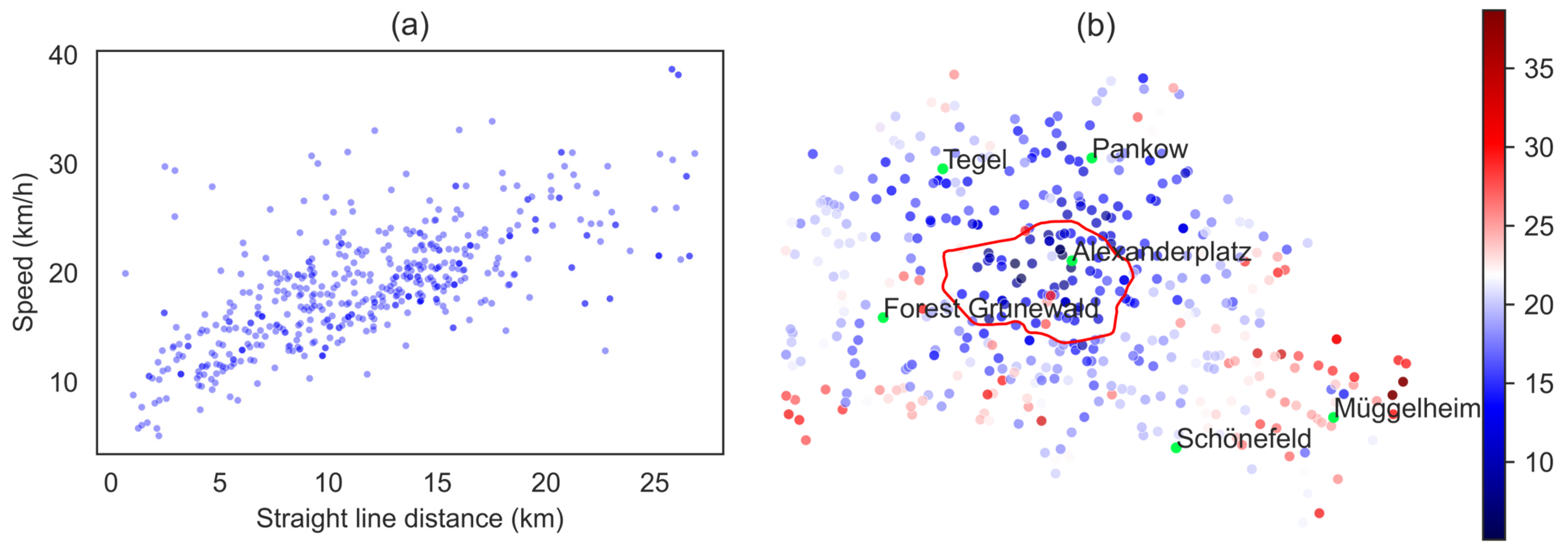
While the distribution is known for the income and commuting distance, only one value for the average speed is known for each city. In order to gain an understanding of variations in public transport speed for different areas within a city, a simulation of Berlin was created: using QGIS (https://www.qgis.org/en/site/, accessed on 17 June 2023), 500 points were randomly placed within the boundaries of Berlin (shapefile source: https://opendata-esri-de.opendata.arcgis.com/datasets/esri-de-content::bezirke-berlin/explore?location=52.510789%2C13.408597%2C10.61, accessed on 17 June 2023). The nearest public transport stops for each of these points were determined using the BVG API (https://v6.bvg.transport.rest, accessed on 13 June 2023 until 15 June 2023). BVG is the public transport operator in Berlin. The travel duration from each of these points to Berlin Friedrichstrasse, a major transport hub in the centre of Berlin, was determined using the BVG API. In order to compare the “average speed” for these trips, the straight-line distance was the most appropriate, as detours would not improve the average speed. It was assumed that the average speed of public transport of all Federal states varies around their respective speeds from the SrV. The spread of the average speed is assumed to be identical to that found in the public transport of Berlin.
‘TomTom’ reports the difference in the travel time inside and outside of rush hour (https://www.tomtom.com/traffic-index/germany-country-traffic/, accessed on 17 June 2023). Based on these data, it was assumed that the average speed of cars follows a normal distribution around the respective mean from the SrV with a sigma of 1.15.
Therefore, people who reported using public transport in the SrV survey may have pre-selected their homes in a convenient location. Car drivers may prefer to live in locations easily accessed by a vehicle. For a solo driver now using public transport, the average speed may be lower compared to someone living in an area optimised for public transport. In the same way, someone living near a public transport hub might face significantly higher costs for parking and reduced speed during rush hour car traffic.
However, this study assumes that everyone is using the quickest mode of transport based on the effective speed. To accommodate the new riders on public transport services would need to be increased. Hopefully, this will result in an adequate public transport service even for those car-dependent neighbourhoods. As this may not be the initial case, a sensitivity analysis was performed where the travel time for public transport was increased by 20%. This accounts for the fact that in rural areas, people may have to adjust their daily activities to match the availability of public transport.
Costs: Defining the cost of owning and operating a car is challenging. If the cheapest car is used, it would not be representative of Germany as most people pay more for their own vehicle. If the average car cost is used, then the fact that a cheaper car could offer the fastest effective speed for some would be ignored. In order to account for this, the study uses the total cost of ownership (TCO) reported by researchers from the Deutsches Zentrum für Luft- und Raumfahrt e.V. (DLR) and Rheinisch-Westfälische Technische Hochschule Aachen (RWTH) [51]. The TCO is reported as EUR/km for various monthly mileage categories. Using a cost per km has the advantage that people with a shorter commute may choose a second hand car, and people with longer commutes may select a newer, more comfortable vehicle. A minimum cost of EUR 8.30 was set to account for the fact that cars have a fixed cost even if they are only used for a km per day. The EUR 8.30 per day is estimated based on the fixed and repair costs reported in the ADAC database [52] for the three most sold cars [53]. Only the cost of the following was included in this study: insurance; tax; oil change; wear and tear repairs (e.g., tiers); and a lump sum of EUR 200 for parking, MOT and small accessories per year. The EUR 8.30 minimum does not include any operating costs (e.g., fuel, oil) nor the depreciation, parking spot at home or at work. ADAC database [52] reports the cost of new cars operated for 5 years. Thus, the assumed wear and tear repairs underestimate the actual repair costs of used cars. In short, the costs assumed in this study very much underestimate the expenditure incurred of car ownership for (i) people who only commute short distances, (ii) people living in cities where they must pay for parking and (iii) well-paid people in cities who may choose an expensive car as their status symbol. In order to account for this, a sensitivity analysis was conducted where the cost per km was assumed to be increased by 20%, and the minimum cost was EUR 20 per day. The EUR 20 is based on an evaluation of mobility costs in Austria [54]. That study concluded that an additional car increases mobility costs by, on average, EUR 5000 per year per household, which corresponds to EUR 22 per working day (assuming 230 working days per year). Bicycle costs were slightly overestimated, as in [16]. The source was [47]. The maximum distance was set to 40 km, given that 30% of people who cycle to work cycle further than 20 km [55]. Walking is free of charge and possible for up to 10 km each day. The costs for Berlin’s monthly public transport ticket were taken from the website of the public transport provider in Berlin VBB [56]. An increased travel distance necessitates a monthly ticket with more zone access to be purchased. Hence, the cost of public transport increases with the travel distance. The average monthly cost of public transport for all other federal states was taken from a statistic by the ADAC [57]. It is assumed that these costs also increase and decrease depending on the travelling distance, similar to the way the public transport cost is changed in Berlin.
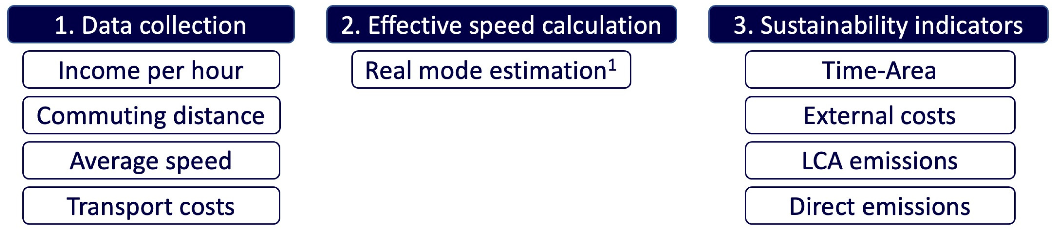
Mode of transport: Obviously, the mode of transport used by the simulated agents ‘in reality’ is unquantified. Only the mode share for each federal state is known [49]. The way the modes of transport were allocated is illustrated in Figure 2. The algorithm starts with allocating everyone the mode of transport they should take based on the effective speed. Since walking was never the best option in this study, the share of people that walk in reality was assumed to be the ones with the shortest commute. In the next step, for each mode of transport, it was checked whether the mode share based on the effective speed was larger than the real mode share. If it was, the agents with the smallest commute were removed. These agents were then allocated to the mode of transport that has a larger share in reality than the share based on the effective speed. The agents with the shortest commute were allocated to cycling, the agents with the next longest trips were given to cars, and the ones with the furthest to public transport.

3.2. Effective Speed

The effective speed is defined as the distance travelled divided by the time required. The time combines the minutes required for the commute and the hours spent earning money for this commute.
E S p e e d = d c h w a g e + t
where:
E S p e e d —Effective speed;
d —average distance travelled per day;
c —total transport cost per day;
h w a g e —hourly after-tax wage;
t —time spent traveling.

3.3. Time–Area Concept

The following equation [31] was used to calculate the time–area requirements (Figure 3).
T A i = l i + s i × t i + t s × d i × w i
where:
T A i —Time–area required for the trip;
l i —Length of the vehicle;
s i —Safety distance between standing vehicles;
d i —Trip distance;
t i —Trip duration;
w i —Width of the lane/right-of-way;
t s —Following rule (usually two seconds).
Figure 3. Specifications of the simulation (source: Schnieder et al. [31]).
Environments 10 00111 g003
The safety distance s i is the minimum distance kept between two parked or stopped vehicles (e.g., at a traffic light). t s is the buffer area kept between two following vehicles in seconds. In most countries around the world, the two-second rule (i.e., distance kept between two moving vehicles) is taught in driving schools or is part of their highway code [58]. More details about the equation and how it was derived can be found in [31]. This equation calculates the legally required area which is required for the transport activity and the duration for which it is used.
Table 1 illustrates the simulation specifications for different modes of transport. In this study, it was assumed that all public transport is performed by bus to simplify the time–area calculation. The assumed occupation of 15 people per 18 m articulated city bus is rather low to ensure that nobody can argue that public transport is only good because ‘too high’ occupancy rates are assumed. The simulation specifications for public transport were estimated so that the resulting time–area requirements are similar to the estimated time–area requirements of various modes of transport in the studies [32,37,38]. Only the time–area requirements while driving were considered, and not while parking. Including this would simply increase the time–area requirements due to overnight parking.

3.4. Emissions

There is a certain level of differentiation between the emission factors for transport activities assumed in various studies. Amongst other factors, this is caused by the difference in the methodologies used to estimate the emission factors [23]. Even small changes in the assumptions can significantly alter the results of an emission simulation [21].
However, the goal was not to quantify the exact emission reductions for a specific context. The concept was rather to use average emission factors, which are representative of a wide range of regions, to estimate possible reductions.
The emission factors used in this study were taken from Mobitool (https://www.mobitool.ch/de/tools/mobitool-faktoren-v2-1-25.html, accessed on 8 April 2023). This is a database of emission factors for 250 different vehicle types. This database is the standard for live cycle assessments in Switzerland. It was chosen despite it not being a perfect match for NYC or Germany, given that the focus was more on a commonly used and validated emission factor database, instead of one that perfectly fits NYC and Germany. A bicycle was used for cycling trips, a large petrol SUV with euro-6b for cars and an 18 m diesel articulated city bus with euro-6 was selected for public transport. The utility of transport was set to 15 people per bus and 1 person for the bicycle and car.

3.5. External Costs

Various methodologies to estimate the external costs have been published over the last few decades [26]. All the external costs used within this study were estimated for a European context as they are a ‘tried and tested’ dataset and are frequently validated and used in similar projections. The datasets and methods have, over 20 years, been continuously updated.
Table 2 depicts the average external costs taken from the ‘Handbook on the External Cost of Transport 2019 Version—1.1′, prepared by CE Delft for the European Union. It is an update of the 2008 and 2014 versions. It mainly focused on external cost figures for European countries. It provides the total external costs, marginal external cost and average external costs of transport. Please refer to the handbook for a detailed overview of the methodology applied. The price level is 2016.
Table 3 shows the external costs estimated as part of a case study in Munich, Germany [26]. Therefore, the results may only be applicable to similar urban environments. It was prepared by academics at the Technical University in Munich. The price level for this study is 2020.
Table 4 illustrates the average external costs in Switzerland. The report was published by the Federal Office for Special Development in Switzerland. It builds up to the method used in the report by Infras and Ecoplan from the 2019 report [59], which provides the external costs from 2010 to 2015. The price level used in this study was 2019.
Based on the above studies, the external costs shown in Table 5 were used in this study. The external cost of public transport and cars are similar to the estimations made by Litman [60] for an American context if only the cost of traffic congestion, barrier effect, crash damages (external), noise pollution, air pollution and resource externalities are considered. If the cost of infrastructure and subsidies are considered as well, the external cost of cars is almost twice as high in Litman [60] than in this study.

3.6. Sensitivity Analysis

As a sensitivity analysis, the results in NYC were compared, assuming that all costs are 20% higher and the travel time is twice as long. People may value the time spent commuting differently compared to working. In order to account for this, the travel time was either halved or doubled. In the sensitivity analysis of the federal states case study in Germany, the cost of cars was increased by 20%, and the public transport travel time was increased by 20%.

3.7. Limitations

The biggest limitation of the study is the cost estimation as well as aggregation based on the federal states in Germany. The cost of owning a car varies greatly between cities and rural areas due to the parking costs. Moreover, well-paid residents in a city might only consider cars that have a certain status symbol, while others traveling between villages might prioritise functionality. Some people who buy used cars may be lucky and do not need to spend much money on repairs, while others may be less fortunate.

4. Results

4.1. New York City

4.1.1. Baseline

Table 6 compares the mode of transport the survey respondents should use with the mode of transport they did use. Only 59% of the survey respondents use the mode of transport they should. Fifty-eight per cent should and do use public transport. Twenty-seven per cent of those who should use public transport drive a car instead. Given that walking was excluded, this does not represent exactly the current mode share based on the number of trips in NYC, from the 2019 survey. Therefore, the mode share by public transport is much higher in this study. For example, person A walks for three trips and takes public transport for two. Person B drives a car for five trips. The resulting trip-based mode share would be 50% car, 30% walking and 20% public transport. In this study, where walking was excluded, and one mode of transport was selected, the mode share would be 50% public transport and 50% car.
Most sustainability indicators reduce when people use the mode of transport with the fastest effective speed (Figure 4). If people chose the fastest mode of transport based on the effective speed, the time–area requirements would reduce by 16%.
The total emissions are based on a life-cycle assessment and include the emissions produced by, for example, the manufacturing of the vehicle. CO2e would reduce by 14.2%, PM10 by 14.7%, PM2.5 by 14.3% and NOx by 12.5%. When only the emissions produced during the operation of the vehicle were compared, the CO2e was reduced by 12.0%. The PM2.5 emissions increased by 10.3%, and the NOx emissions also increased by 3.4%. This is due to the NOx and PM2.5 emissions being higher for public transport than during the operation of private cars. The external costs reduce by 11.6% if users can use the mode of transport they should, compared to the mode of transport they used in reality.

4.1.2. Sensitivity Analysis

Table 7 lists the reduction in emissions, time–area requirements and external costs for the baseline and the sensitivity analysis. By increasing the cost of transport by 20%, the time–area requirements can be reduced by 22.9%, which is a further reduction of 6.4 per cent points (pp). The external costs would reduce by 16.6%, which is a 5 pp further decrease than the baseline. The total emission reduction increases by a further 5.9 pp to 6.7 pp. If the travel time is considered double compared to the time spent working, almost no reductions can be observed (<5%). On the other hand, these factors reduce by up to 33.4% if it is assumed that the time spent commuting is only half as long as the time spent working.

4.2. Germany

4.2.1. Mode Share

The results are aggregated for the sixteen federal states in Germany. An overview of these can be seen in Table 8.
Figure 5 illustrates the variation in the speed of public transport (i.e., straight-line distance/travel duration). The average is 18.6 km/h (0.1 percentile: 12 km/h; 0.9 percentile: 25.8 km/h). This is faster than the average speed by public transport according to the SrV in Berlin (i.e., 15.1 km/h), as no walking distance is included. This confirms that the speed of public transport differs depending on the location. However, the average speed of cars varies in a similar way depending on the time of the day and/or day of the week, according to TomTom (https://www.tomtom.com/traffic-index/berlin-traffic/, accessed on 17 June 2023). The average speed ranges between 21 km/h and 39 km/h in the centre of Berlin and between 33 km/h and 50 km/h in the metro area.
The mode share for commuting trips in reality and based on the effective speed is compared in Figure 6. In the baseline scenario, the mode share for cars is higher in reality than it is suggested based on the effective speed. It ranges from 39% to 83% in reality and 2% to 50% based on the effective speed. The mode share for bicycles ranges from 2% to 20% in reality and 2% to 20% based on the effective speed. Public transport is slightly more attractive in reality than cycling, with 6% to 42% and 22% to 87% based on the effective speed.
In scenario b, where the cost of owning a car is increased, driving is rarely the fastest option. The mode share for cars reduces to between 0% and 14%. Public transport gains the most from an increased car cost (48% to 91%). The mode share for bicycles stays almost the same at 2% to 30%.
Increasing the travel time by public transport (scenario c) reduces its mode share to between 4% and 73%. While the mode share for cars is still lower than in reality, it increases to between 15% and 60%. The mode share for cycling increases to between 2% and 34%.

4.2.2. External Costs, Emissions and Time–Area Requirements

Figure 7 shows the possible reduction in the external costs, emissions and time–area requirements if people choose the quickest mode of transport based on the effective speed. The external effects of transport can, for most Federal States, be reduced if the best mode of transport based on the effective speed is chosen. In scenario a (baseline), the biggest reduction in the time–area requirements (51%), external costs (43%) and LCA emissions (49% to 54%) can be achieved by Brandenburg. Similar to the NYC case study, the direct PM2.5 and NOx emissions increased in this case study due to the increased usage of public transport. For the majority of Federal States, the possible time–area reduction is around 15%, and the external costs are reduced by around 16%. The LCA emissions for the majority of the Federal States are reduced by around 18%.
In scenario b, the reductions are even more pronounced. Brandenburg is again showing the largest potential reductions with similar values. The average reductions are 29% for the time–area requirements, 33% for the external costs and around 39% for the LCA emissions.
In scenario c, Berlin and Hamburg are worse off, if everyone uses the fastest mode of transportation based on the effective speed. For the majority of Federal States, the time–area requirements and external costs reduce by around 5% and around 7%. The LCA emissions for the majority of the Federal States are reduced by around 7%. Given that public transport is not attractive anymore in Hamburg and Berlin in scenario c, the direct PM2.5 and NOx emissions reduce by between 2 and 13%.

5. Discussion

In contrast to the case study of the Federal States in Germany, the case study in NYC uses the mode of transport the survey respondents chose and their actual income and travel distance. In the NYC case study, only 59% of the survey respondents use the fastest mode of transport based on the effective speed (RO1). Twenty-seven per cent of those who should use public transport drive a car instead. A 16.5% reduction in the time–area requirements can be achieved if the survey respondents had chosen the mode of transport they should instead of the one they did (RO2). The external costs could be reduced by 11.6%, and the LCA emissions could be reduced by 12.5–14.7%. If the costs of all modes of transport are increased by 20%, then larger reductions are possible, as more people should use public transport or bicycles based on the effective speed. If the travel time is doubled, traveling by car becomes the better choice for more survey respondents, and the possible reductions are less than 5%. If the travel time is halved, even further reductions could be possible.
In the case study of the Federal States in Germany, the mode share for cars, in reality, is higher than the suggested mode share based on the effective speed (RO3). If people chose their fastest mode of transport based on the effective speed, most federal states are generally better off. For the majority of Federal States, the possible time–area reduction is around 15%, and around 16% for the reduction in the external costs (RO4). The LCA emissions for the majority of the Federal States are reduced by around 18%.
The results are as expected. Given that people generally underestimate the cost of car ownership, it is not surprising that some underestimate the amount of time they spend earning money to pay for their daily commute. The study also shows that reducing the average speed of public transport in Germany by just 20% has a substantial negative impact on the economic attractiveness of sustainable modes of transport. This highlights that the quality of public transportation is key to achieving sustainability goals. Increasing the average speed may not be the only option to increase the effective speed of public transport. Enabling people to use their time productively (e.g., relaxing, working) on public transport may be a way to save time.

6. Conclusions and Future Work

Instead of trying to invent new technologies and policies, or inconveniencing people by asking them to forgo their travel needs, alternative ideas to reduce the external effect of traffic are the focus of this study. In order to reduce global warming, this paper estimates the possible reductions in the external effects without asking people to spend more money on new technologies or more time on their transport activities. Instead, this paper proposes to encourage people to simply use the fasted mode of transport based on the effective speed. Effective speed considers both the time spent commuting as well as the time spent earning the money to pay for it.
In the NYC case study, a 16.5% reduction in the time–area requirements can be achieved if the survey respondents had chosen the mode of transport they should use instead of the one they used. The external cost could be reduced by 11.6%, and the LCA emissions could be reduced by 12.5–14.7%.
In the case study of the Federal States in Germany, the mode share for cars, in reality, is much higher than the suggested mode share based on the effective speed. It ranges from 39% to 83% in reality and 2% to 50% based on the effective speed. For the majority of federal states, the time–area requirements reduce by around 15% and around 16% for the reduction in external costs. The LCA emissions for the majority of the federal states are reduced by around 18%.
The NYC case study is based on actual survey respondents, while the case studies of the Federal States in Germany are a simulation based on statistical evidence. Hence, future work would ideally validate the simulation based on a larger-scale survey.
The results of this paper highlight that people may not need to spend more time or money on their transport activity to travel in a more sustainable way. Instead, encouraging people to use a mode of transport with a faster effective speed may reduce the external effects for some.
This study clearly highlights that a sizable reduction in sustainability indicators can be achieved by simply encouraging people to choose the mode of transport that has the highest effective speed. The study shows that sustainable modes of transport are the most cost-effective for the less affluent. Offering this demographic an attractive public transport system and cycling infrastructure should be of the utmost importance for policymakers. It not only saves time and money for the lower income groups—it gives them more freedom and is also good for the planet. As a consequence, it frees up space on the roads for wealthy residents, for whom it may not be an economical choice to ride a bicycle or use public transport.
Future research should focus on how to use the effective speed concept in the real world. How can those who would save time and money by using bicycles or public transport be encouraged? Which factors prevent them from achieving this, and which factors encourage them? Future work should investigate the best mode share based on the effective speed for a wider cohort of cities. Comparisons should be made between those cities well known for their sustainable modes of transport alongside car-dependent environments with limited public transport service. A theoretical study optimising the transport infrastructure and services to maximise effective speed may then be of high interest to policymakers. An evaluation of the effective speed of mobility as a service (MaaS) as well as shared mobility could drive future policies.

Funding

This research received no external funding.

Data Availability Statement

Emissions and LCA: Mobitool https://www.mobitool.ch/de/tools/mobitool-faktoren-v2-1-25.html, accessed on 1 April 2023). Travel and household data: NYC Open Data, “Citywide Mobility Survey—Household Survey 2019,” 2022. [Online]. Available online: https://data.cityofnewyork.us/api/odata/v4/a5rk-jemi, accessed on 7 April 2023. NYC Open Data, “Citywide Mobility Survey—Trip Survey 2019,” 2022. https://data.cityofnewyork.us/api/odata/v4/w9dc-u4ik (accessed on 7 April 2023). NYC Open Data, “Citywide Mobility Survey—Person Survey 2019,” 2022. [Online]. Available online: https://data.cityofnewyork.us/Transportation/Citywide-Mobility-Survey-Person-Survey-2019/6bqn-qdwq, accessed on 7 April 2023.

Conflicts of Interest

The author declare no conflict of interest.

References

  1. Schnieder, M.; Hinde, C.; West, A. Land consumption of delivery robots and bicycle couriers for on-demand meal delivery using gps data and simulations based on the time-area concept. Sustainability 2021, 13, 11375. [Google Scholar] [CrossRef]
  2. Zhou, J.; Chang, S.; Ma, W.; Wang, D. An unbalance-based evaluation framework on urban resources and environment carrying capacity. Sustain. Cities Soc. 2021, 72, 103019. [Google Scholar] [CrossRef]
  3. Da Silva, T.B.; Baptista, P.; Silva, C.A.S.; Santos, L. Climate change mitigation policies in the transportation sector in Rio de Janeiro, Brazil. Environments 2020, 7, 99. [Google Scholar] [CrossRef]
  4. De Luca, G.; Pizzolante, F.; Petracchini, F.; Paolini, V.; Rizza, V.; Kim, K.-H. Detecting Leaders Country from Road Transport Emission Time-Series. Environments 2021, 8, 18. [Google Scholar] [CrossRef]
  5. Paulino, F.; Pina, A.; Baptista, P. Evaluation of alternatives for the passenger road transport sector in Europe: A life-cycle assessment approach. Environments 2018, 5, 21. [Google Scholar] [CrossRef] [Green Version]
  6. Gunawan, H.; Bressers, H.; Mohlakoana, N.; Hoppe, T. Incorporating air quality improvement at a local level into climate policy in the transport sector: A case study in Bandung City, Indonesia. Environments 2017, 4, 45. [Google Scholar] [CrossRef] [Green Version]
  7. Tang, J.; McNabola, A.; Misstear, B.; Caulfield, B. An evaluation of the impact of the Dublin Port Tunnel and HGV management strategy on air pollution emissions. Transp. Res. D Transp. Environ. 2017, 52, 1–14. [Google Scholar] [CrossRef]
  8. Ramacher, M.O.P.; Matthias, V.; Aulinger, A.; Quante, M.; Bieser, J.; Karl, M. Contributions of traffic and shipping emissions to city-scale NOx and PM2.5 exposure in Hamburg. Atmos Environ. 2020, 237, 117674. [Google Scholar] [CrossRef]
  9. Cappelletti, G.M.; Grilli, L.; Russo, C.; Santoro, D. Sustainable mobility in universities: The case of the university of foggia (Italy). Environments 2021, 8, 57. [Google Scholar] [CrossRef]
  10. Tranter, P.J.; May, M. Questioning the need for speed: Can ‘effective speed’ guide change in travel behaviour and transport policy? Australas. Transp. Res. Forum 2005, 28, 15. [Google Scholar]
  11. Litman, T. Not So Fast: Better Speed Valuation for Transportation Planning. 2021. Available online: https://vtpi.org/nsf.pdf (accessed on 7 April 2023).
  12. Tranter, P. Effective Speeds: Car Costs are Slowing us Down. Australian Greenhouse Office. 2004. Available online: https://citeseerx.ist.psu.edu/document?repid=rep1&type=pdf&doi=616342a78d237767c1e2462c648cb62961ebbb6b (accessed on 7 April 2023).
  13. Illich, I. Energy and Equity; Harper & Row: New York, NY, USA, 1974. [Google Scholar]
  14. Tranter, P.J.; May, M. The Hidden Benefits of Walking: Is speed Stealing Our Time and Money? In Walk 21-VII The Next Steps. In Proceedings of the 7th International Conference on Walking and Liveable Communities, Melbourne, Australia, 23–25 October 2006; Available online: www.walk21.com (accessed on 7 April 2023).
  15. Kifer, K. Auto Costs Versus Bike Costs. 2004. Available online: https://www.phred.org/~alex/kenkifer/www.kenkifer.com/bikepages/advocacy/autocost.htm (accessed on 7 April 2023).
  16. Tranter, P.J. Effective Speed: Cycling because it’s faster. In City Cycling; MIT Press: Cambridge, MA, USA, 2012; p. 57. [Google Scholar]
  17. Meira, L.H.; de Mello, C.A.; Castro, Y.M.; Oliveira, L.K.; de Oliveira Leite Nascimento, C. Measuring social effective speed to improve sustainable mobility policies in developing countries. Transp. Res. D Transp. Environ. 2020, 78, 102200. [Google Scholar] [CrossRef]
  18. Sims, D.B.; Hudson, A.C.; Park, J.H.; Hodge, V.; Porter, H.; Spaulding, W.G. Buellia dispersa (Lichens) used as bio-indicators for air pollution transport: A case study within the las vegas valley, nevada (USA). Environments 2017, 4, 94. [Google Scholar] [CrossRef] [Green Version]
  19. Jursova, S.; Burchart-Korol, D.; Pustejovska, P. Carbon footprint and water footprint of electric vehicles and batteries charging in view of various sources of power supply in the Czech Republic. Environments 2019, 6, 38. [Google Scholar] [CrossRef] [Green Version]
  20. Corazza, M.V.; Di Mascio, P.; Esposito, G. Airports as Sensitive Areas to Mitigate Air Pollution: Evidence from a Case Study in Rome. Environments 2022, 9, 108. [Google Scholar] [CrossRef]
  21. Schnieder, M.; Hinde, C.; West, A. Sensitivity analysis of emission models of parcel lockers vs. Home delivery based on hbefa. Int. J. Environ. Res. Public Health 2021, 18, 6325. [Google Scholar] [CrossRef] [PubMed]
  22. Schnieder, M.; Hinde, C.; West, A. Emission Estimation of On-Demand Meal Delivery Services Using a Macroscopic Simulation. Int. J. Environ. Res. Public Health 2022, 19, 11667. [Google Scholar] [CrossRef]
  23. Salini, R.; Lenngren, C.A.; Bassi, L.; Baesso, D.P. Greenhouse gas assessment and compensation on Brazilian low volume rural roads using carbonroad—The santa rosa de lima case. Environments 2015, 2, 489–499. [Google Scholar] [CrossRef] [Green Version]
  24. Christine Externe Kosten und Nutzen des Verkehrs in der Schweiz. Available online: https://www.are.admin.ch/are/en/home/mobility/data/costs-and-benefits-of-transport.html (accessed on 2 April 2023).
  25. Verhoef, E. External effects and social costs of road transport. Transp. Res. Part A 1994, 28, 273–287. [Google Scholar] [CrossRef]
  26. Schröder, D.; Kirn, L.; Kinigadner, J.; Loder, A.; Blum, P.; Xu, Y.; Lienkamp, M. Ending the myth of mobility at zero costs: An external cost analysis. Res. Transp. Econ. 2022, 97, 101246. [Google Scholar] [CrossRef]
  27. Euchi, J.; Kallel, A. Internalization of external congestion and CO2 emissions costs related to road transport: The case of Tunisia. Renew. Sustain. Energy Rev. 2021, 142, 110858. [Google Scholar] [CrossRef]
  28. Essen, H.; Fiorello, D.; El Beyrouty, K.; European Commission Directorate-General for Mobility and Transport. Handbook on the External Costs of Transport: Version 2019-1.1, Publications Office, 2020. 2019. Available online: https://data.europa.eu/doi/10.2832/51388 (accessed on 11 October 2021).
  29. Lavee, D. Land use for transport projects: Estimating land value. Land Use Policy 2015, 42, 594–601. [Google Scholar] [CrossRef]
  30. Zheng, N.; Geroliminis, N. On the distribution of urban road space for multimodal congested networks. Transp. Res. Part B Methodol. 2013, 57, 326–341. [Google Scholar] [CrossRef] [Green Version]
  31. Schnieder, M.; Hinde, C.; West, A. Review and development of a land consumption evaluation method based on the time-area concept of last mile delivery using real delivery trip data. Sustainability 2020, 12, 626. [Google Scholar] [CrossRef]
  32. Bruun, E.C. Calculation and Evaluation of the Time-Area Parameter for Different Transportation Modes; University of Pennsylvania, ProQuest Dissertations Publishing: Philadelphia, PA, USA, 1992; Available online: https://search.proquest.com/docview/303998393?accountid=12152 (accessed on 20 April 2020).
  33. Montgomery, C. Happy City: Transforming Our Lives Through Urban Design; Penguin: London, UK, 2013. [Google Scholar]
  34. Milosavljevic, N.; Simicevic, J. Sustainable Parking Management: Practices, Policies, and Metrics; Elsevier: Amsterdam, The Netherlands, 2019. [Google Scholar] [CrossRef]
  35. Schnieder, M.; Hinde, C.; West, A. Land Efficient Mobility: Evaluation of Autonomous Last Mile Delivery Concepts in London. Int. J. Environ. Res. Public Health 2022, 19, 10290. [Google Scholar] [CrossRef] [PubMed]
  36. Schnieder, M.; Hinde, C.; West, A. Land Efficient Mobility and Emissions: Click and Collect vs. Grocery Deliveries in Switzerland. Sustainability 2023, 15, 8814. [Google Scholar] [CrossRef]
  37. Brunner, H.; Hirz, M.; Hirschberg, W.; Fallast, K. Evaluation of various means of transport for urban areas. Energy Sustain. Soc. 2018, 8, 9. [Google Scholar] [CrossRef] [Green Version]
  38. Shin, Y.E.; Vuchic, V.R.; Bruun, E.C. Land consumption impacts of a transportation system on a city. Transp. Res. Rec. 2009, 2110, 69–77. [Google Scholar] [CrossRef]
  39. Litman, T. Transportation Land Valuation Evaluating Policies and Practices that Affect the Amount of Land Devoted to Transportation Facilities. Victoria Transport Policy Institute. 2018. Available online: https://www.vtpi.org/land.pdf (accessed on 18 March 2023).
  40. Vale, D. Effective accessibility: Using effective speed to measure accessibility by cost. Transp. Res. D Transp. Environ. 2020, 80, 102263. [Google Scholar] [CrossRef]
  41. NYC Open Data Citywide Mobility Survey—Household Survey 2019. 2022. Available online: https://data.cityofnewyork.us/api/odata/v4/a5rk-jemi (accessed on 7 April 2023).
  42. NYC Open Data Citywide Mobility Survey—Trip Survey 2019. 2022. Available online: https://data.cityofnewyork.us/api/odata/v4/w9dc-u4ik (accessed on 7 April 2023).
  43. NYC Open Data Citywide Mobility Survey—Person Survey 2019. 2022. Available online: https://data.cityofnewyork.us/Transportation/Citywide-Mobility-Survey-Person-Survey-2019/6bqn-qdwq (accessed on 7 April 2023).
  44. Schnieder, M. Effective Speed: Factors That Influence the Attractiveness of Cost Effective and Sustainable Modes of Transport in Cities. Sustainability 2023, 15, 8338. [Google Scholar] [CrossRef]
  45. Gosine, S. Is It Worth Owning a Car in NYC? 2020. Available online: https://www.hauseit.com/owning-a-car-nyc/#Traffic%20&%20Parking%20Tickets (accessed on 7 April 2023).
  46. AAA Your Driving Costs 2021—How Much Does it Really Cost to Own a New Car? 2021. Available online: https://newsroom.aaa.com/wp-content/uploads/2021/08/2021-YDC-Brochure-Live.pdf (accessed on 7 April 2023).
  47. DieEinsparBerater OHG Kosten-, Zeit- und Verbrauchsvergleich Verschiedener Fahrradtypen. Available online: http://www.dieeinsparinfos.de/guenstige-mobilitaet/fahrrad/kosten/ (accessed on 7 April 2018).
  48. Statistisches Bundesamt (Destatis) Ergebnis 12211-1003-DLAND. Bevölkerung, Erwerbstätige, Erwerbslose, Erwerbspersonen, Nichterwerbspersonen aus Hauptwohnsitzhaush.: Bundesländer, Jahre, Geschlecht, Größenkl. Persönl. Monatl. Nettoeinkommen. 2023. Available online: https://www-genesis.destatis.de/ (accessed on 7 April 2023).
  49. Bauer-Hailer, U. Berufspendler im Bundesländervergleich. Stat. Mon. Baden-Württemberg 2019, 2, 10–14. Available online: https://www.statistik-bw.de/Service/Veroeff/Monatshefte/PDF/Beitrag19_02_02.pdf (accessed on 7 April 2023).
  50. Gerike, R.; Hubrich, S.; Ließke, F.; Wittig, S.; Wittwer, R. Tabellen zum Forschungsprojekt Mobilität in Städten—SrV 2018. Available online: https://tu-dresden.de/bu/verkehr/ivs/srv/ressourcen/dateien/SrV2018_Ergebnispraesentation.pdf?lang=en (accessed on 8 April 2020).
  51. Eisenmann, C.; Tobias, I.; Berlin, K. Für Vielfahrer oft Konkurrenzlos Günstig: Pkw-Nutzung in Deutschland. 2019. Available online: http://www.verkehrskonferenz.de/fileadmin/archiv/konferenz_2019/praesentationen/Verkehrskonferenz_2019_FR_9.00_2035_eisenmann.pdf (accessed on 7 April 2023).
  52. ADAC ADAC Autokosten Frühjahr/Sommer 2023 Kostenübersicht für Über 1.500 Aktuelle Neuwagen-Modelle. 2023. Available online: https://assets.adac.de/Autodatenbank/Autokosten/autokostenuebersicht.pdf (accessed on 7 May 2023).
  53. Beliebteste Automodelle 2022|Statista. Available online: https://de.statista.com/statistik/daten/studie/3149/umfrage/automodelle-mit-den-meisten-neuzulassungen-in-deutschland/#:~:text=Der%20VW%20Golf%20war%202022,der%20VW%20Golf%20am%20beliebtesten (accessed on 7 April 2023).
  54. Madlener, D.J. Kosten von Alltagsmobilität für Haushalte in Vorarlberg. Technischen Universität Wien. 2018. Available online: http://www.ub.tuwien.ac.at/eng (accessed on 8 April 2023).
  55. Fakten, Z.U. Studie zur Allgemeinen Fahrradnutzung in Deutschland; Fahrrad: Stuttgart, Germany, 2015. [Google Scholar]
  56. VBB VBB-Umweltkarte. 2023. Available online: https://www.vbb.de/en/tickets/monthly-tickets/vbb-umweltkarte/ (accessed on 7 April 2023).
  57. ADAC. ÖPNV Ticketvergleich: Gewaltige Preisunterschiede|ADAC. 4 November. 2021. Available online: https://www.adac.de/reise-freizeit/ratgeber/tests/oepnv-preisvergleich/ (accessed on 7 April 2023).
  58. TG Road Safety Safe Distance between Vehicles. CEDR Report 402 2009/10.1. 2010. Available online: https://www.cedr.eu/download/Publications/2010/e_Distance_between_vehicles.pdf (accessed on 8 May 2020).
  59. Lieb, C.; Sommer, H.; Amacher, M. Externe Effekte des Verkehrs 2015. Available online: www.infras.ch (accessed on 5 March 2023).
  60. Litman, T.A.; Litman, T. Transportation Cost Estimates. 2022. Available online: www.vtpi.org/tca (accessed on 5 March 2023).
  61. Statistisches Bundesamt (Destatis). Result 12211-9004-DLAND—Population, Persons in Employment, Unemployed Persons, Economically Active Population, Economically Inactive Population: Länder, Years (until 2019). 2021. Available online: https://www-genesis.destatis.de/genesis/online?operation=abruftabelleBearbeiten&levelindex=1&levelid=1685633268512&auswahloperation=abruftabelleAuspraegungAuswaehlen&auswahlverzeichnis=ordnungsstruktur&auswahlziel=werteabruf&code=12211-9004&auswahltext=&wertauswahl=78&wertauswahl=57&wertauswahl=58&wertauswahl=56&wertauswahl=343&werteabruf=Value+retrieval#abreadcrumb (accessed on 7 April 2023).
  62. Statistisches Bundesamt (Destatis). Result 11111-0001-DLAND—Size of Territory: Länder, Reference Date. 2021. Available online: https://www-genesis.destatis.de/genesis/online?operation=abruftabelleBearbeiten&levelindex=1&levelid=1685632753161&auswahloperation=abruftabelleAuspraegungAuswaehlen&auswahlverzeichnis=ordnungsstruktur&auswahlziel=werteabruf&code=11111-0001&auswahltext=&werteabruf=Value+retrieval#abreadcrumb (accessed on 7 April 2023).
  63. Statistisches Bundesamt (Destatis). Result 12411-0050-DLAND—Population Density: Länder, Reference Date. 2021. Available online: https://www-genesis.destatis.de/genesis/online?operation=abruftabelleBearbeiten&levelindex=1&levelid=1685632125853&auswahloperation=abruftabelleAuspraegungAuswaehlen&auswahlverzeichnis=ordnungsstruktur&auswahlziel=werteabruf&code=12411-0050&auswahltext=&werteabruf=Value+retrieval#abreadcrumb (accessed on 8 April 2023).
Figure 1. Methodology applied in this study. (1 Step not required for the NYC case study as the data are known).
Environments 10 00111 g001
Figure 2. Mode share allocation.
Environments 10 00111 g002
Figure 4. Change in per cent of survey respondents using the fastest mode of transport based on the effective speed.
Environments 10 00111 g004
Figure 5. (a) The ‘speed’ of public transport in Berlin, defined as a straight line distance to the city centre is divided by the travel duration. (b) A map of Berlin depicting the origin of 500 trips taken to the city centre and the colour of each dot depicts the ‘speed’ for the trip (red line: Ringbahn—German for circle railway).
Environments 10 00111 g005
Figure 6. Comparison of the real mode share and the quickest mode share based on the effective speed: (a) baseline; (b) increased car costs; (c) 20% increased travel time by public transport.
Environments 10 00111 g006aEnvironments 10 00111 g006b
Figure 7. Change in the emissions, time–area requirements and external costs if people select the mode of transport with the highest effective speed: (a) baseline; (b) increased car costs; (c) 20% increased travel time by public transport.
Environments 10 00111 g007
Table 1. Simulation specifications (source: Schnieder et al. [31] for bicycle and car/taxi).
l i s i w i t s Occupancy
Bicycle1.801.50.033333331
Car and Taxi4.412.750.033333331
Public transport (Bus)1232.750.110
Table 2. Average external costs (price level 2016) for EU28 passenger transport (selected modes of transport) (adopted from [28]).
Passenger CarBusHigh-Speed TrainElectric TrainDiesel Train
Cost CategoryEUR-cent/pkmEUR-cent/pkmEUR-cent/pkmEUR-cent/pkmEUR-cent/pkm
Accidents4.51.00.10.50.5
Air Pollution0.70.80.00.00.8
Climate1.20.50.00.00.3
Noise0.60.40.30.81.4
Congestion4.20.8
Well-to-Tank0.40.20.30.80.1
Habitat damage0.50.10.60.60.8
Total12.03.71.32.63.9
Table 3. Average external costs (price level 2020) (selected modes of transport) (adopted from [26]).
Bus DieselTramSubwayRegional TrainCar DieselCar GasolineBicycle
EUR-cent/Pkm11.368.013.994.6216.9715.96.72
Table 4. External costs in Switzerland Rp. pro Pkm (price level 2019) [24].
Mode of TransportPassenger CarVeloBusTrolleyTram
Health damage due to air pollution2.36 4.25
Building damage due to air pollution0.17 0.31
Crop failures due to air pollution0.03 0.09
Forest damage due to air pollution0.03 0.06
Biodiversity loss due to air pollution0.08 0.14
Damage due to noise1.16 2.170.100.17
Climate costs1.28 1.41
Damage to nature and landscape0.830.490.460.050.02
Ground damage0.08 0.210.110.00
Costs from upstream and downstream processes0.941.100.560.420.71
Accident costs0.3820.740.150.000.12
Costs in urban areas0.03 0.020.020.02
Total7.3622.339.810.701.04
External health benefits of non-motorised traffic 18.24
Table 5. External costs assumed in this study in euro cents per pkm.
Car, TaxiBus/Public TransportBicycleWalking
11.935.015.414.76
Table 6. Mode of transport the survey respondents should use vs. mode used (N = 2501) (same as in [44]).
Should/IsTaxiBikeCarPublic TransportSum
Taxi0%0%0%0%0%
Bike1%0%2%5%8%
Car0%0%1%1%2%
Public Transport2%3%27%58%90%
Sum3%3%30%64%100%
Table 7. Reduction in emissions if people use the mode of transport they should.
Base LineCost IncreaseTravel Time IncreaseTravel Time Reduction
Time–area16.522.94.533.4
External costs11.616.62.324.6
CO2e Total14.220.81.731.8
PM10 Total14.721.32.132.3
PM2.5 Total14.320.82.031.6
NOx Total12.518.41.328.3
CO2e Direct12.017.81.027.4
PM2.5 Direct10.3 *13.5 *5.0 *17.9 *
NOx Direct3.4 *3.8 *3.1 *3.9 *
* Emissions increase and do not reduce.
Table 8. Federal states in Germany (source: [61,62,63]).
Population Density (inh./km2)Size of Territory (sq km2)PopulationPersons in Employment
10001000
Baden-Württemberg31135,747.8210,9635987
Bayern18670,541.5712,9077076
Berlin4112891.1236041868
Brandenburg8529,654.3524711244
Bremen1621419.62676332
Hamburg2453755.091827979
Hessen29821,115.6462013220
Mecklenburg-Vorpommern6923,295.451580761
Niedersachsen16847,709.8278454017
Nordrhein-Westfalen52534,112.4417,6658807
Rheinland-Pfalz20619,85840172090
Saarland3832571.11972478
Sachsen22018,449.9340071985
Sachsen-Anhalt10720,459.1221591027
Schleswig-Holstein18415,804.328511465
Thüringen13116,202.3921021042
Disclaimer/Publisher’s Note: The statements, opinions and data contained in all publications are solely those of the individual author(s) and contributor(s) and not of MDPI and/or the editor(s). MDPI and/or the editor(s) disclaim responsibility for any injury to people or property resulting from any ideas, methods, instructions or products referred to in the content.

