Analysis of Uncertainty in the Depth Profile of Soil Organic Carbon

Abstract

The soil organic carbon (SOC) depth profile provides information for many applications, including monitoring climate change, carbon sequestration, reforestation, and land erosion. Models of the SOC profile support data interpolation, trend analysis, and carbon mapping, and can be used in larger pedometric models in support of carbon farming. Model errors may be due to statistical variability in discrete data and the limited sample size available for model calibration. Uncertainties in the model can arise from a process of iterative parameter adjustment and can be estimated by gradient-based methods or probabilistic methods. A comparison between Frequentist and Bayesian approaches to the construction of regression-based models revealed that the results were very similar when used for calibrating a model for the SOC profile. The model was applied to four representative regional sites in Victoria.

1. Introduction

Soil organic carbon (SOC) is an important property of soil that generally decreases with depth. Understanding the nature of SOC stores in the soil and the changes over time is a subject gaining increasing attention in the contexts of sustainability, climate change, carbon sequestration, and landscape management [1]. The estimation of SOC profiles is relevant to monitoring soil condition and land use change over space and time, and for monitoring climate change and the design of sequestration strategies, as soils are both a source and sink of CO₂. Recent research has revealed that soils may release more CO₂ than originally expected as deeper soil layers are affected by global warming, leading to increasing estimates of emissions by as much as 34 to 37 percent over non-warmed soil [2]. The Victorian Government website lists 70 links to references on soil carbon and emissions (https://agriculture.vic.gov.au/climate-and-weather, accessed on 25 October 2022).

In the context of the modelling and simulation of the SOC profile depth, errors in a model can be due to parameter uncertainty, but also includes model structure adequacy, measurement errors, and a variety of epistemic uncertainties that have been identified [3,4]. Statistical uncertainty is not just due to measurement error recorded from in situ experimental replications, but also includes limited sample size and variability in the model inputs and parameters. Error propagation may be important in large and complex systems as represented by soil attribute models, and ecosystems [5,6,7,8,9,10].

The aim of this pilot study was (a) to compare Frequentist and Bayesian approaches when applied to a simple power law model for the SOC depth profile using representative field data from regional Victoria, and (b) to fit the power law model to SOC profiles to four regional locations with different soil types to evaluate performance.

2. Materials and Methods

2.1. Bayesian Regression

In model calibration, the coefficients of an arbitrary non-linear model are adjusted in order to minimise the difference between model predictions and experimental measurements, i.e., to minimise the objective function, S(${\theta }_1$,${\theta }_2$), which is the sum-of-squared errors between model predictions, f_i (${\theta }_1$,${\theta }_2$), and experimental values, y_i, as follows,

$$S\left({\theta }_1,{\theta }_2\right)=\sum _{i=1}^n{(y_i-f_i\left({\theta }_1,{\theta }_2\right))}^2$$

(1)

Probabilistic methods for calibration offer an alternative to deterministic error minimisation procedures based on gradient (calculus) approaches, mainly because they incorporate more detailed treatment of uncertainty.

The Bayesian Inference approach combines Bayes Law with Monte Carlo simulation in a process known as Markov Chain Monte Carlo (MCMC) simulation, where sampling is carried out iteratively from probability distributions [11,12].

The prior information provided for the parameters or inputs may be realistic estimates of lower and upper bounds, or the nature and shape of the probability distribution, or both, insofar as this information aids in defining the feasible parameter space $\theta \in {\Re }^n$ [13].

The Bayesian approach is described by the following brief review of the defining equations. Using the formalism of [14], given p model parameters, $\theta :\left({\theta }_1,\dots ,{\theta }_p\right)$ with prior information, and a set of observations on the p parameters, $x:\left(x_1,\dots ,x_m\right)$, the dependence of the observations on the parameters is expressed by the likelihood function, p(x|θ), or L(θ|x), and the posterior probability distribution of the parameter, $\theta$, given the observed data, x, as follows [14,15],

$$p\left(\theta \left|x\right.\right)=\frac{p(x\left|\theta )p\left(\theta \right)\right.}{\int p(x\left|\theta )p\left(\theta \right)d\theta \right.}$$

(2)

noting that $\theta$ is a random variable representing the parameter, where the x represents the observed data, $p(\theta \left|x)\right.$ is the posterior distribution, and $p\left(\theta \right)$ is the prior distribution.

The likelihood function may have uncorrelated normally distributed residuals, with variance ${\sigma }^2$; i.e., the general form for the computation is along the following lines for parameter $\theta$,

$$p(x\left|\theta )\equiv \right.L(\theta \left|x_1,\dots ,x_m)=\right.\prod _{i=1}^m{f}_x\left(x_i\left|\theta \right.\right)$$

(3)

where L(θ|x₁, …, x_m) is the likelihood function, which is defined as follows,

$$L(\theta \left|x_1,\dots ,x_m)=\right.\prod _{i=1}^m\frac{1}{\sqrt{2\pi {\sigma }^2}}\exp \left[-\frac{{(x_i-x_i\left(\theta \right))}^2}{{\sigma }^2}\right]$$

(4)

where the Box–Cox transform is used to ensure the residuals follow the normal probability distribution [16].

The posterior parameter distribution, $p(\theta \left|x)\right.$, is estimated by the method of Markov Chain Monte Carlo (MCMC) simulation, using sampling schemes based on the Metropolis–Hastings or Gibbs algorithms [11,17].

2.2. Deterministic Error Analysis

For parameter estimation in regression models, there is the problem of error propagation between inputs and outputs. The error, σ, is a classical measure of uncertainty and for deterministic models can be estimated by differential calculus. For fixed coefficients in a mathematical model or equation [18], the predictive model y = f(x) is a mapping in the real domain f: ${\Re }^n\to \Re$ for an n-dimensional input such that the inputs or parameters are a multi-dimensional quantity. If the function is smooth, continuous, and differentiable, the Taylor series approximation to the function y is

$$y\left(x\right)\cong y\left(x_0\right)+\sum _{i=1}^n\left[\frac{\partial f\left(x_0\right)}{\partial x_i}\right]\left(x_i-x_{i0}\right)$$

(5)

where the variance, σ²(y), is given by

$${\sigma }^2\left(y\right)=\sum _{i=1}^n{\left[\frac{\partial f\left(x_0\right)}{\partial x_i}\right]}^2{\sigma }^2\left(x_i\right)$$

(6)

The contributions to output error from the inputs are weighted by their partial derivatives. A covariance term is added if there is correlation between variables [18,19,20,21].

Some disadvantages of the differential approach are that the approximation breaks down when the function contains discontinuities, step functions, undefined points or regions, or conditional logic branches. Furthermore, only first- and second-order moments of the output distribution are produced, not the entire probability distribution. The normal approximation for the error distribution is assumed.

An uncertainty metric often used is the normalised standard deviation, i.e., the coefficient of variation, CV, where the ratio is the relative or normalised error (standard deviation) adjusted for the magnitude of input [22]. The gain factor, G, for uncertainty propagation is the ratio of the output CV to the input CV,

$$G=\frac{C{V}_{output}}{C{V}_{input}} \mathrm{where} CV=\frac{\sigma \left(X\right)}{\overline{X}}$$

(7)

The gain, G, is a metric for the magnitude of error propagation through the model.

2.3. SOC Depth Profile

In pedology, assessment of soil organic carbon (SOC) stocks is important for many reasons, including monitoring climate change and the design of sequestration strategies, as soils are both a source and sink of CO₂. Assessment of SOC stocks are also relevant to monitoring soil condition and land use, and management of change over space and time. Estimates of SOC are subject to uncertainty and increasingly there are efforts to quantify errors in estimates under different conditions [23,24,25,26]. One approach is to calculate SOC stock by a relationship such as the following,

$$y=f\left(x\right)=\frac{x_1{x}_2{x}_3\left(1-x_4\right)}{100}$$

(8)

where y is the SOC stock (t C ha⁻¹), x₁ is the SOC depth profile (m), x₂ is SOC concentration (g C kg⁻¹), x₃ is bulk density (kg m⁻³), and x₄ is proportion of large fragments (rock) and is dimensionless [27].

Examination of empirical data collected in this study suggested that a power law model may be an adequate model for representing the soil organic carbon depth profile, especially in south-eastern Australia. This finding was consistent with another study that also found that soil organic carbon levels varied according to land use, being lowest in farmland and higher in woodland [28]. Below 60 cm, the differences between land use categories were smaller, as the carbon content is determined mainly by the root system distribution. In each case, the measured data in their study indicated a monotonically decreasing function with sampling depth that could be approximated by a power law model.

Uncertainty can be quantified by first-order differential error analysis (Equation (6)), or Monte Carlo simulation, assuming no significant correlation between the variables. Recently, different researchers [27,29] studied the problem of correlation between variables and included the covariance terms in the Taylor series approximation (Equations (5) and (6). This results in the following expression for variance in the case of Equation (8),

$${\sigma }^2\left(y\right)=\sum _{i=1}^n{\left[\frac{\partial f\left(x_0\right)}{\partial x_i}\right]}^2{\sigma }^2\left(x_i\right)+2\sum _{i=1}^n\sum _{j=i+1}^n\left[\frac{\partial f\left(x_0\right)}{\partial x_i}\right]\left[\frac{\partial f\left(x_0\right)}{\partial x_j}\right] Cov\left(x_i,x_j\right)$$

(9)

Consistent with the notation in this paper, the sum of variances and covariances for the SOC stock estimate [27] can now be expressed as follows,

$$\begin{gathered} {\sigma }_y^2\approx \left[\frac{{\sigma }_{x_1}^2}{x_1^2}+\frac{{\sigma }_{x_2}^2}{x_2^2}+\frac{{\sigma }_{x_3}^2}{x_3^2}+\frac{{\sigma }_{x_4}^2}{{(1-x_4)}^2}+2\frac{{\sigma }_{x_1{x}_2}}{x_1{x}_2}+2\frac{{\sigma }_{x_1{x}_3}}{x_1{x}_3}+2\frac{{\sigma }_{x_{2}x{3}_3}}{x_2{x}_3}\right. \\ \left.-2\frac{{\sigma }_{x_1\left(1-x_4\right)}}{{x_1}_{(1-x_4)}}-2\frac{{\sigma }_{x_2\left(1-x_4\right)}}{{x_2}_{(1-x_4)}}-2\frac{{\sigma }_{x_3\left(1-x_4\right)}}{{x_3}_{(1-x_4)}}\right]y^2 \end{gathered}$$

(10)

where the first four terms are the variances, and the remaining six terms are the covariances. One researcher [27] noted that covariances are often not included in such assessments, with only the simplified form of the delta rule being used [29]. In this paper, the interest is in the SOC depth profile given by x₁ in Equation (8) and we also assume negligible correlation with the other variables.

3. Results

This section provides a concise description of the experimental results, their interpretation, as well as the experimental conclusions that can be drawn.

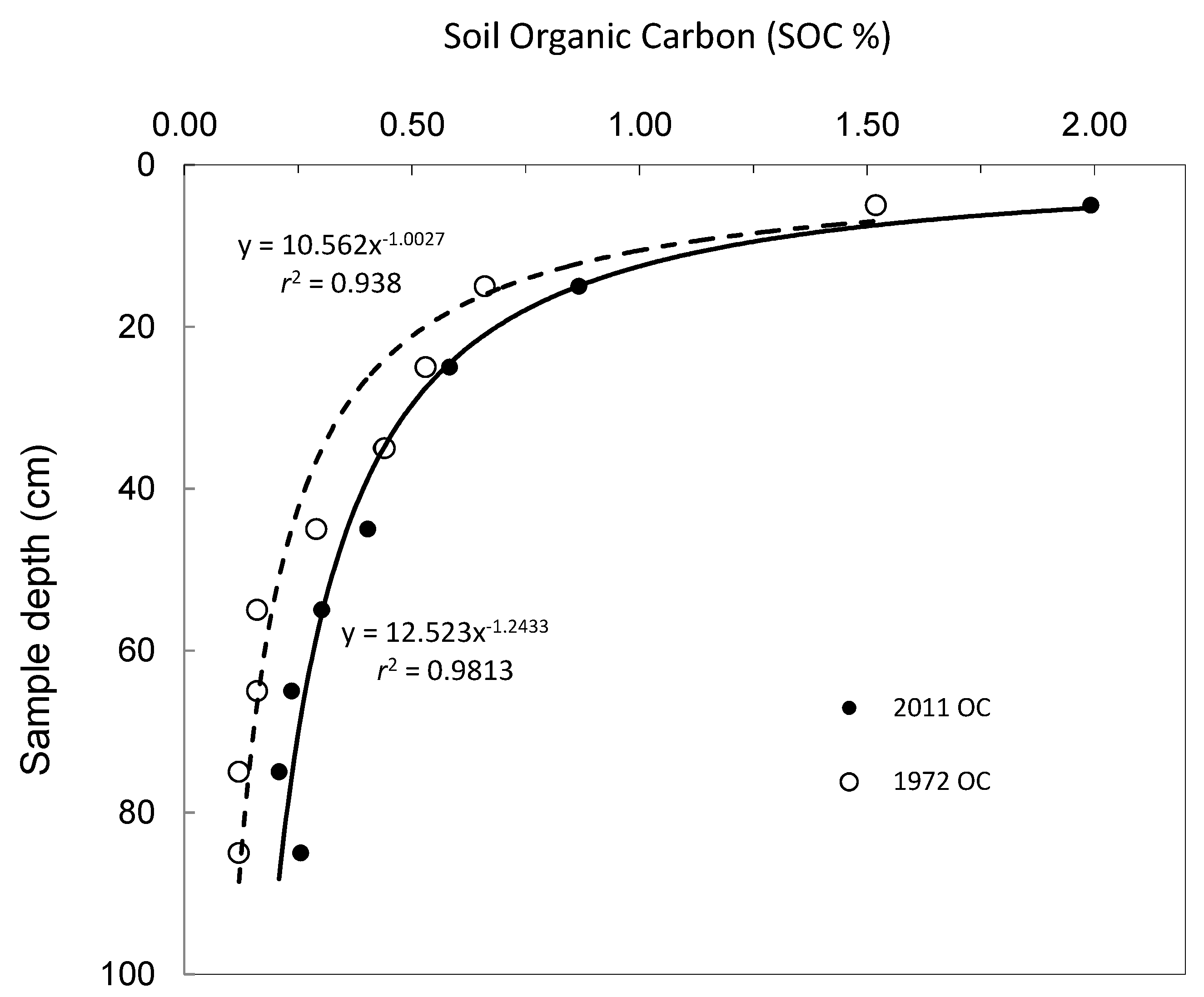
3.1. Deterministic Regression Model

The decrease in SOC content with the soil depth variable, x₁, is depicted by the scatterplot in Figure 1. The scatterplot shows data for SOC, from samples taken in 1972 and 2011 in south-western Victoria and analysed for temporal variability using the published Walkley–Black method [30]. From empirical studies by the authors using Victorian data on carbon depth profiles, the relationship follows the general form of a power law (also later supported by [28]). That is, for a specified set of conditions, one can express y as the level of SOC at depth x₁, such that

$$y=f\left(x_1\right)={\theta }_1{x_1}^{-{\theta }_2}$$

(11)

Power law functions are used to model many natural processes and are distinguished by their scale invariance, which is the reason for their central role in, for example, fractal analysis (note that the model is described by the scale parameter ${\theta }_1$, and the shape parameter ${\theta }_2$). Applying Equation (6) to Equation (11) for differential error analysis together with algebraic manipulation results in

$$\frac{{\sigma }_y}{y}={\theta }_2\frac{{\sigma }_{x_1}}{x_1}$$

(12)

or, expressed in the form of the uncertainty transfer function approach,

$$C{V}_y={\theta }_{2}C{V}_{x_1}$$

(13)

from which it is evident that the shape parameter ${\theta }_2$ alone determines the magnitude and amplification factor for the transfer of uncertainty from input to output in the model.

With respect to the difference in the two scatterplots in Figure 1, one may assess the significance by using the parametric paired t-test for observations with the null hypothesis H₀: μ₁ − μ₂ = µ_D [22]. A two-sided test produced borderline significance for µ_D (p = 0.015) with 95% CI = [0.03648, 0.2480]. The application of the Wilcoxon non-parametric paired test also reveals no significant difference between the two profiles for a two-sided test. These results suggest that over the period between sampling, the statistical difference in the profiles may not be significant.

There may be additional uncertainty introduced when a predictive model is constructed based on least-squared error analysis using a scatterplot of data. The curve fits in Figure 1 were completed using a standard spreadsheet function (Microsoft Excel 2003), based on classical regression analysis, assuming no significant error in the independent variable. In addition, the data was fitted a second time, more accurately, by non-linear regression analysis using the Levenberg–Marquardt technique for error minimisation [31].

The scaling parameter was determined as ${\theta }_1$ = 6.925, the shape parameter as ${\theta }_2$ = 0.7729, and the regression statistics as: r² = 0.9977, d.f. adjusted r² = 0.9969, fit s.e. = 0.0291, s.e. (${\theta }_1$) = 0.2352, s.e. (${\theta }_2$) = 0.01512, and F-value = 3025.5. The analysis was repeated for the 1972 dataset, with the scaling parameter determined as ${\theta }_{1 }$= 5.329, the shape parameter as ${\theta }_2$ = 0.7729, and the regression statistics as: r² = 0.9786, d.f. adjusted r² = 0.9715, fit s.e. = 0.0701, s.e. (${\theta }_1$) = 0.5663, s.e. (${\theta }_2$) = 0.04734, and F-value = 320.2. (Note: d.f. adjusted r² = (1 – SSE × (n − 1) / SSM × (df − 1)), which follows Equation (12) in [32].)

The confidence intervals for the parameters for the 2012 data were also computed as 95% CI (${\theta }_1$) = [6.367, 7.484], and 95% CI (${\theta }_2$) = [0.737, 0.809], and for the 1972 data as 95% CI (${\theta }_1$) = [3.984, 6.673], and 95% CI (${\theta }_2$) = [0.661, 0.885]. The experimental results reveal that the shape parameter, ${\theta }_2$, has increased slightly the magnitude of error propagated, in contrast to the use of the error-free value of ${\theta }_2$. This example illustrates the point that model fitting to a scatterplot, by regression analysis, may add regression error to the total error propagated through the model. In addition, the variability in the output (CV_y) is 77% of the variability in the input (CV_x1) due to the compressive effect of the model structure during error propagation.

Note also, from the plot in Figure 1, that the older 1972 plot is nearly a lateral translation of the 2011 plot, indicating a lower level of carbon at the various depths in 1972 (The exception is at the 5 cm depth for the older data, where there is a single anomalous point, which may be an artefact—an observation supported by a visual inspection of the trend line and scatterplot). This result suggests that the underlying physical processes involved in the carbon attenuation with depth have not changed significantly over time.

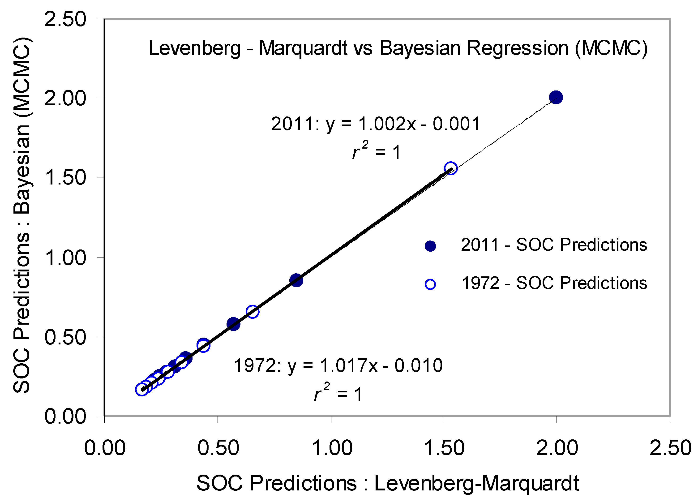
3.2. Comparison with Bayesian Regression

The power law fit can also be estimated within a Bayesian framework, where the parameters are represented as probability distributions rather than point estimates [33]. In this approach, the parameter distributions are determined using Bayes Law, combining field measurements with prior information available on the parameters [15,34].

The Bayesian regression approach was applied to the power law, with a total of 10,000 trials for the burn-in period and 100,000 trials for the simulation. An uninformed prior (i.e., initial uniform distribution) was used together with the Gibbs sampling scheme. The determination of the coefficients for the power law model showed strong agreement between the Levenberg–Marquardt (LM) error-minimisation scheme and the Bayesian regression, as can be observed in Figure 2 and

Table 1. Comparison of Frequentist and Bayesian regression results for parameter uncertainty for SOC depth profile (based on parameters ${\theta }_1$ and ${\theta }_2$ in the Power Law function).

Date	Parameter	Frequentist	Bayesian	Excel 2003
(Year)		(Levenberg–Marquardt)	(MCMC)	(Transform)
2011	${\theta }_1$	6.925	6.948	7.241
	${\theta }_2$	0.773	0.774	0.789
1972	${\theta }_1$	5.329	5.518	8.435
	${\theta }_2$	0.773	0.787	0.936

. The fit standard error for the LM method was 0.029 (2011 SOC data) and 0.070 (1972 SOC data).

The scatter point at a 5 cm depth for the 1972 legacy data appears to have affected the results for the LM method. In contrast, the Bayesian posterior standard deviations for the model output were 0.036 (2011 SOC data) and 0.032 (1972 SOC data). The Bayesian approach is more conservative in comparison with respect to the more recent, higher quality, 2011 SOC data. This is explained by different definitions on uncertainty intervals and modelling assumptions (e.g., treating the parameters as distributions rather than fixed values and constraint relaxation with respect to the normal distribution).

Frequentist and Bayesian regression approaches produced strong agreement in the determination of the model coefficients for the power law. The uncertainty intervals, however, in the model outputs are slightly different, being more conservative in the Bayesian case due to different parameter definitions and assumptions in the analysis.

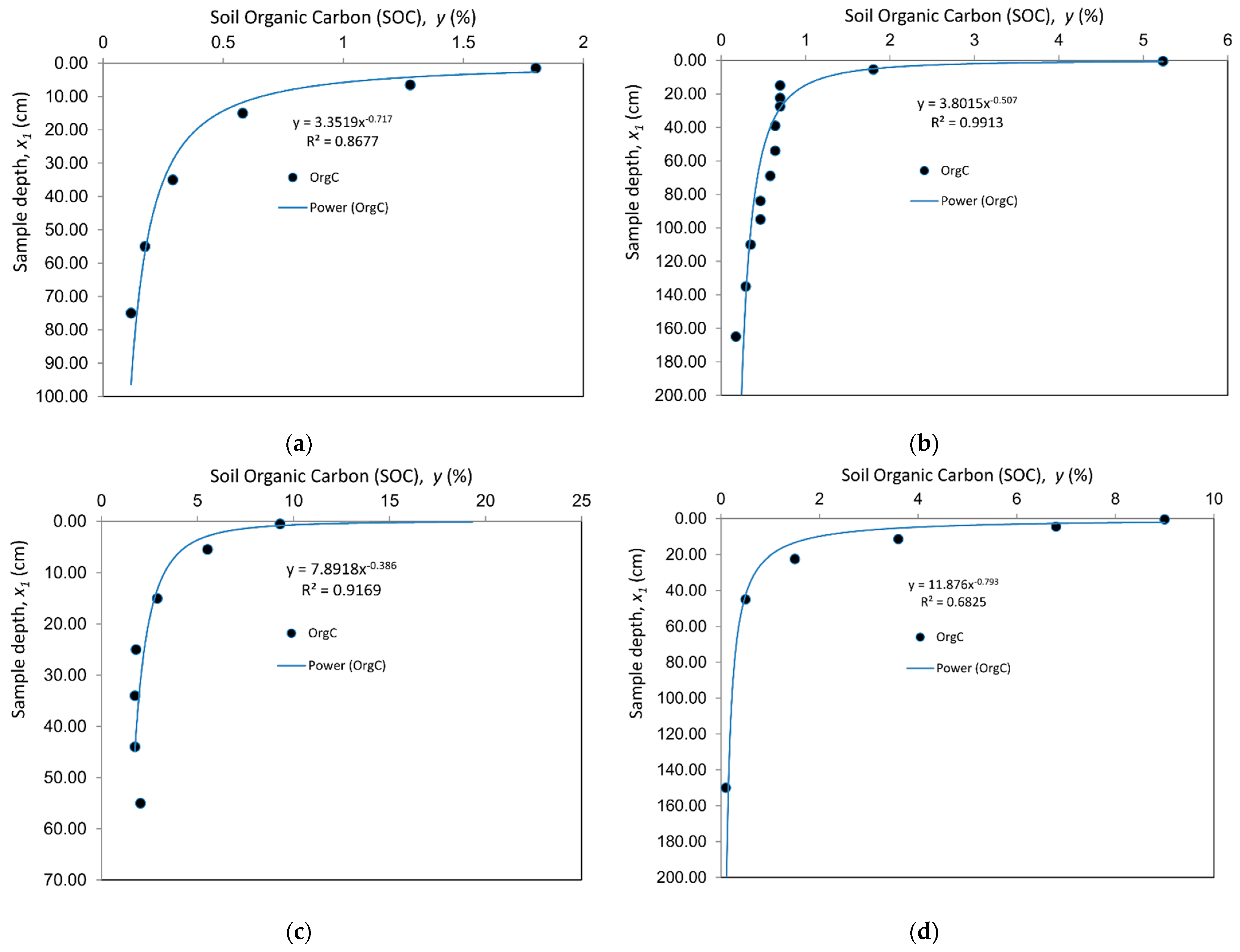
3.3. Application to Regional Data

The power law function represented by Equation (11) was applied to new data from four locations in regional Victoria, each with a different soil type. The scatterplots were fitted using the standard regression modelling function using the Excel spreadsheet option and the results are depicted in Figure 3a–d. All four locations and soil types yielded very good fits to the model: namely, Wimmera: Vertosol, r² = 0.86773; Boorook: Sodosol, r² = 0.9913; Girringurrup: Dermosol, r² = 0.9169; and Wangerrip: Rudosol, r² = 0.6825.

All four results have correlation coefficients that are statistically significant relative to the sample size (p < 0.05). Visual confirmation of all scatterplots confirmed very good fitting performance.

4. Discussion

The level of organic carbon in soil has a significant impact on soil health and the health of landscapes and catchments. It is now recognised that the exchange of carbon between the atmosphere and soil is an important aspect of the global carbon cycle. Carbon levels in the soil can be affected by bushfires, grazing animals, and large-scale deforestation. More specifically, soil carbon content can be increased by decomposing organic matter from plants and animals and also biochar. Declines in the historic levels of SOC have often been caused by the mismanagement of agricultural systems, such as over-grazing or over-harvesting, and the effects of pollution. The organic carbon present in the soil can vary considerably, from peaty soils where organic carbon can be greater than 10%, to less than 1% in heavily tilled dryland soils [35]. Increases in organic carbon can have important benefits to the physical, chemical, and biological function of the medium that may extend deeper into the profile for perennial pasture or high rainfall settings [36]. Knowledge of the organic carbon content at depth can also be important for understanding nutrient cycling and balances and primary productivity [37].

There is continuing research on the strategy and effectiveness of sequestration of atmospheric carbon dioxide in soil to mitigate the effects of climate change. Soil organic matter cycling depends on the soil type, climate, and farm management, with rainfall as an important driver of plant growth, and the subsequent decomposition of organic matter in the soil (see https://www.agric.wa.gov.au) (accessed on 25 October 2022). Different types of soil organic matter (e.g., particulate, humus, resistant, or dissolved) can change at various rates, also known as turnover time [37]. The organic matter in the soil cycles constantly between living, decomposing, and stable proportions where various microorganisms digest most of the organic carbon in the soil, transferring the carbon back into the atmosphere as carbon dioxide [36].

The SOC depth profile model provides a tool and metric for the assessment of the levels of subsoil organic carbon, over time and space, subject to different soil properties and environmental conditions. A regression model of the SOC depth profile enables predictions at different depths of interest for which measurements were not available and is a means of monitoring over time to compare various mitigation strategies.

The SOC depth profile may vary at different locations subject to several factors, such as the type and density of vegetation and various biochemical processes occurring at different soil depths (such as at the root zone).

For the power law model, both classical regression analysis and Bayesian regression produced coefficients and model fitting accuracy with good agreement. The uncertainty intervals were similar in the case of the 2011 data, with the Bayesian model being slightly more conservative. For the 1972 data, fitting accuracy was again similar, but the uncertainty (fit standard error) was less using Bayesian regression.

The advantage of model fitting by deterministic regression is that it is in widespread use. However, the treatment of uncertainty in estimates is more limited when compared with Bayesian approaches [10,11,31]. Probabilistic regression using Bayesian inference allows for incorporating uncertainty analysis in the parameter estimation and the possibility of providing prior information, such as error distributions for the parameter’s initial estimates [11,12,13,14,15].

A disadvantage of Bayesian regression is the approach is much more computationally intensive and, in some applications, prior information based on expert opinion has been described as subjective by frequentist statisticians. Although the differences in uncertainty estimation were not very great for the more modern 2011 data, the Bayesian approach has potential in that it can be developed further to include epistemic uncertainty in the inputs in a systematic manner (using probability distributions rather than fixed values).

With respect to error propagation, the results have the following salient features:

(a)

When the power law model is used with error-free coefficients, the transfer of uncertainty (σ or CV) is entirely determined by the exponent, i.e., the coefficient ${\theta }_2$ as demonstrated mathematically by differential error analysis.

(b)

If a model is fitted to the scatterplot by regression, there is added uncertainty due to errors in the estimation of the coefficients. Once again, only the shape coefficient ${\theta }_2$ for the power law model matters and not the scaling coefficient, ${\theta }_1$. In the latter case, only a translation is involved with the scaling coefficient, ${\theta }_1$.

There are several insights gained from this study. First, the power law model appears to be appropriate to characterise the SOC profile of different soil types at different locations. Second, a classical regression approach is sufficient for the purpose of parameter estimation. Third, a frequentist approach provides good accuracy in estimates of the SOC profile without undue computational expense. This is an important consideration for monitoring by soil analysts for those who may not have the knowledge or software to carry out Bayesian analysis.

In the case of routine sampling of SOC at regional locations, the SOC profile model may be used to estimate SOC levels at depths not conventionally measured. For example, the power law function could be used to estimate carbon concentrations at specific depths that are important to researchers, such as 10cm or 30cm, at a large range of locations and so provide three-dimensional maps that can be compared over time (four-dimensional).

A future challenge is to apply the model over as many regional locations and soil types as possible and to check for changes in the profile over time, either in magnitude or shape. This may provide evidence associated with the stability of soil organic carbon levels in response to management or climatic impacts. The simplicity of the model allows for the easy incorporation into larger models supporting climate change studies. For example, the model may be used as a tool to compare interventions that may affect soil carbon storage, such as reforestation potential.

5. Conclusions

Modelling the soil organic carbon profile was conducted using a power law fitted to scatterplots of field data from different regional soil types in Victoria. The model calibration was investigated using deterministic non-linear regression (Levenberg–Marquardt gradient approach for error minimisation) and probabilistic regression in the form of Bayesian inference (MCMC simulation). The results of this study support the hypothesis that (a) the power law can be used for modelling the SOC profile for different types of regional soils, and (b) the two calibration methods used are similar in accuracy.

The power law function for SOC depth profiles can be applied to the development of 3D maps of the carbon composition in regional areas. The SOC model can also be recalibrated over multiple time-steps to support studies in soil carbon change over time and the sequestration performance evaluated for comparing reforestation strategies. The Bayesian approach has greater computational expense and complexity but can incorporate prior error distributions from previous analysis.

References

1. Biggs, A.J.W.; Grundy, M.J. The need for better links between pedology and soil carbon research in Australia. Soil Res. 2010, 48, 1–6. [Google Scholar] [CrossRef]
2. Hicks Pries, C.E.; Castanha, C.; Porras, R.; Torn, M.S. The whole-soil carbon flux in response to warming. Science 2007, 355, 1420–1423. [Google Scholar] [CrossRef]
3. Refsgaard, J.C.; van der Sluijs, J.P.; Højberg, A.L.; Vanrolleghem, P.A. Uncertainty in the environmental modelling process—A framework and guidance. Environ. Model. Softw. 2007, 22, 1543–1556. [Google Scholar] [CrossRef]
4. Robinson, N.J.; Benke, K.K.; Norng, S. Identification and interpretation of sources of uncertainty in soils change in a global systems-based modelling process. Soil Res. 2015, 53, 592–604. [Google Scholar] [CrossRef]
5. Heuvelink, G.B.M.; Burrough, P.A. Developments in statistical approaches to spatial uncertainty and its propagation. Int. J. Geog. Inf. Sci. 2002, 16, 111–113. [Google Scholar] [CrossRef]
6. Brown, J.D.; Heuvelink, G.B.M. Assessing Uncertainty Propagation Through Physically based Models of Soil Water Flow and Solute Transport. In Encyclopedia of Hydrological Sciences; Anderson, M., McDonnell, J., Eds.; Wiley & Sons: Chichester, UK, 2005. [Google Scholar]
7. Hamilton, A.J.; Basset, Y.; Benke, K.K.; Grimbacher, P.S.; Miller, S.E.; Novotný, V.; Samuelson, G.A.; Stork, N.E.; Weiblen, G.D.; Yen, J.D. Quantifying uncertainty in estimation of tropical arthropod species richness. Am. Nat. 2010, 176, 90–95. [Google Scholar] [CrossRef] [PubMed]
8. Hamilton, A.J.; Novotny, V.; Waters, E.K.; Basset, Y.; Benke, K.K.; Grimbacher, P.S.; Miller, S.E.; Samuelson, G.A.; Weiblen, G.D.; Yen, J.D.; et al. Estimating global arthropod species richness: Refining probabilistic models using probability bounds analysis. Oecologia 2013, 171, 357–365. [Google Scholar] [CrossRef] [PubMed]
9. Benke, K.K.; Robinson, N.J. Quantification of Uncertainty in Mathematical Models: The Statistical Relationship between Field and Laboratory pH Measurements. Appl. Environ. Soil Sci. 2017, 2017, 1–12. [Google Scholar] [CrossRef]
10. Benke, K.K.; Norng, S.; Robinson, N.J.; Benke, L.R.; Peterson, T.J. Error propagation in computer models: Analytic approaches, advantages, disadvantages and constraints. Stoch. Environ. Res. Risk Assess. 2018, 32, 2971–2985. [Google Scholar] [CrossRef]
11. Kuczera, G.; Parent, E. Monte Carlo Assessment of Parameter Uncertainty in Conceptual Models: The Metropolis Algorithm. J. Hydrol. 1998, 211, 69–85. [Google Scholar] [CrossRef]
12. Kavetski, D.; Kuczera, G.; Franks, S.W. Bayesian Analysis of Input Uncertainty in Hydrological Modelling: 1. Theory. Water Resour. J. 1998, 42, W03407. [Google Scholar]
13. Vrugt, J.A.; Gupta, H.V.; Bouten, W.; Sorooshian, S. The Shuffled Complex Evolutionary Metropolis Algorithm for optimisation and uncertainty assessment of hydrological parameters. Water Resour. Res. 2003, 39, 1201. [Google Scholar] [CrossRef]
14. Qian, S.S.; Stow, C.A.; Borsuk, M.E. On Monte Carlo Methods for Bayesian inference. Ecol. Model. 2003, 159, 269–277. [Google Scholar] [CrossRef]
15. Carlin, B.P.; Louis, T.A. Bayesian Methods for Data Analysis, 3rd ed.; Chapman and Hall: Boca Raton, FL, USA, 2008. [Google Scholar]
16. Box, G.E.P.; Cox, D.R. An analysis of transformations revisited, rebutted. J. Amer. Stat. Assoc. 1982, 77, 209–210. [Google Scholar] [CrossRef]
17. Geman, S.; Geman, D. Stochastic Relaxation, Gibbs Distributions, and the Bayesian Restoration of Images. IEEE Tran. Pattern Anal. Mach. Intell. 1984, 6, 721–741. [Google Scholar] [CrossRef] [PubMed]
18. Helton, J.C. Uncertainty and Sensitivity Analysis Techniques for Use in Performance Assessment for Radioactive Waste Disposal. Reliab. Eng. Syst. Saf. 1993, 42, 327–367. [Google Scholar] [CrossRef]
19. Mandel, J. The Statistical Analysis of Experimental Data; Dover Publications Inc.: New York, NY, USA, 1984. [Google Scholar]
20. Parratt, L.G. Probability and Experimental Errors in Science; Dover Publications Inc.: New York, NY, USA, 1971. [Google Scholar]
21. Taylor, J.R. An Introduction to Error Analysis; University Science Books: Sausalito, CA, USA, 1997. [Google Scholar]
22. Freund, J.E. Mathematical Statistics; Prentice-Hall: Englewood Cliffs, NJ, USA, 1971. [Google Scholar]
23. McBratney, A.B. On variation, uncertainty and informatics in environmental soil management. Aust. J. Soil Res. 1992, 30, 913–935. [Google Scholar] [CrossRef]
24. Bishop, T.F.A.; Minasny, B.; McBratney, A.B. Uncertainty analysis for soil-terrain models. Int. J. Geog. Inf. Sci. 2006, 20, 117–134. [Google Scholar] [CrossRef]
25. Heuvelink, G.B.M. Realistic quantification of input, parameter and structural errors of soil process models. In Proceedings of the Solutions for a Changing World, 19th World Congress of Soil Science, Brisbane, Australia, 1–6 August 2010. [Google Scholar]
26. Malone, B.P.; McBratney, A.B.; Minasny, B. Empirical estimates of uncertainty for mapping continuous depth functions of soil attributes. Geoderma 2011, 160, 614–625. [Google Scholar] [CrossRef]
27. Goidts, E.; van Wesmael, B.; Crucifix, M. Magnitude and sources of uncertainties in soil organic carbon (SOC) stock assessments at various scales. Eur. J. Soil Sci. 2009, 60, 723–729. [Google Scholar] [CrossRef]
28. Li, M.; Zhang, X.; Pang, G.; Han, F. The estimation of soil organic carbon distribution and storage in a small catchment area of the Loess Plateau. Catena 2013, 101, 11–16. [Google Scholar] [CrossRef]
29. Panda, D.K.; Singh, R.; Kundu, D.K.; Chakraborty, H.; Kumar, A. Improved Estimation of Soil Organic Carbon Storage Uncertainty Using First-Order Taylor Series Approximation. Soil Sci. Soc. Am. J. 2008, 72, 1708–1711. [Google Scholar] [CrossRef]
30. Rayment, G.E.; Lyons, D.J. Soil Chemical Methods: Australia; CSIRO Publishing: Collingwood, Australia, 2011. [Google Scholar]
31. Gill, P.E.; Murray, W.; Wright, M.H. The Levenberg-Marquardt Method. In Practical Optimization; Academic Press: London, UK, 1981. [Google Scholar]
32. Kvålseth, T.O. Cautionary note about R 2. Am. Stat. 1985, 39, 279–285. [Google Scholar] [CrossRef]
33. Bayes, T. An essay towards solving a problem in the doctrine of chances. Phil. Trans. Roy. Soc. Lond. 1763, 53, 1393–1442. [Google Scholar] [CrossRef]
34. Freni, G.; Mannina, G. Bayesian approach for uncertainty quantification in water quality modelling: The influence of prior distribution. J. Hydrol. 2010, 392, 31–39. [Google Scholar] [CrossRef]
35. Robertson, F.; Crawford, D.; Partington, D.; Oliver, I.; Rees, D.; Aumann, C.; Armstrong, R.; Perris, R.; Davey, M.; Moodie, M.; et al. Soil organic carbon in cropping and pasture systems of Victoria, Australia. Soil Res. 2016, 54, 64–77. [Google Scholar] [CrossRef]
36. Hoyle, F.C.; D’Antuono, M.; Overheu, T.; Murphy, D.V. Capacity for increasing soil organic carbon stocks in dryland agricultural systems. Soil Res. 2013, 51, 657–667. [Google Scholar] [CrossRef]
37. Murphy, B.W. Impact of soil organic matter on soil properties—A review with emphasis on Australian soils. Soil Res. 2015, 53, 605–635. [Google Scholar] [CrossRef]
Figure 1. Soil organic carbon content (SOC) as a function of soil depth in 1972 and 2011 in a designated sample site in south-western Victoria.
Environments 10 00029 g001
Figure 2. Levenberg–Marquardt error-minimisation regression model vs. Bayesian regression (MCMC) shows good agreement in SOC model predictions using the power law function.
Environments 10 00029 g002
Figure 3. SOC models: (a) Vertosol profile (site A978) from the Wimmera; (b) Sodosol profile (site 485) from Boorook (south-western Victoria); (c) Dermosol profile (site 488) at Girringurrup (south-western Victoria); (d) Rudosol profile (site OTR426) from Wangerrip (Otway Ranges). Note that SOC models are presented with axes (x and y) reversed for display purposes.
Environments 10 00029 g003