

Mass-Movement Causes and Landslide Susceptibility in River Valleys of Lowland Areas: A Case Study in the Central Radunia Valley, Northern Poland


Abstract
:1. Introduction
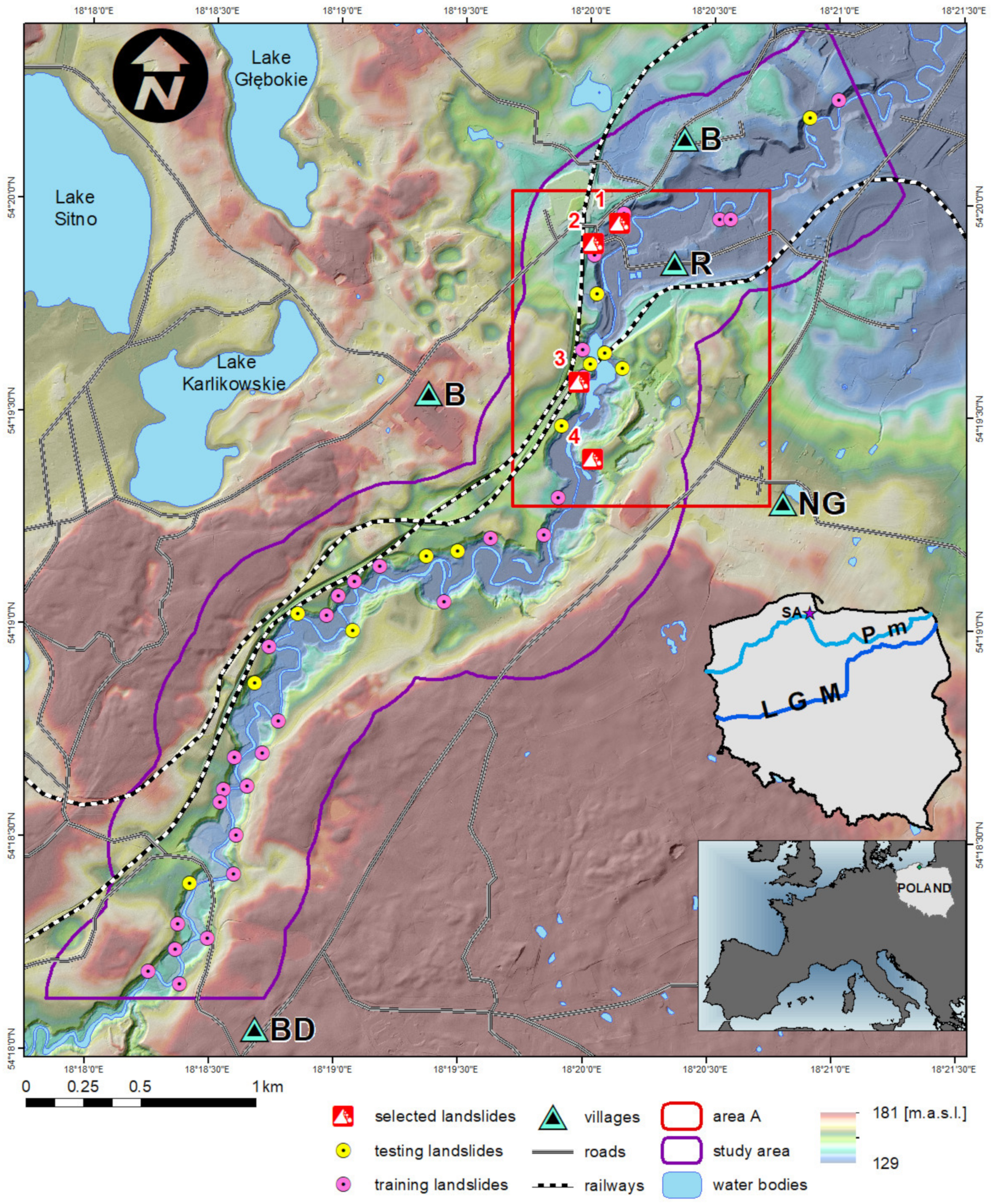
Study Area
2. Materials and Methods
2.1. Analysis of the Rutki Landslide
2.2. Susceptibility Assessment of the Central Radunia Valley
3. Results
3.1. Landslides in the Central Radunia Valley
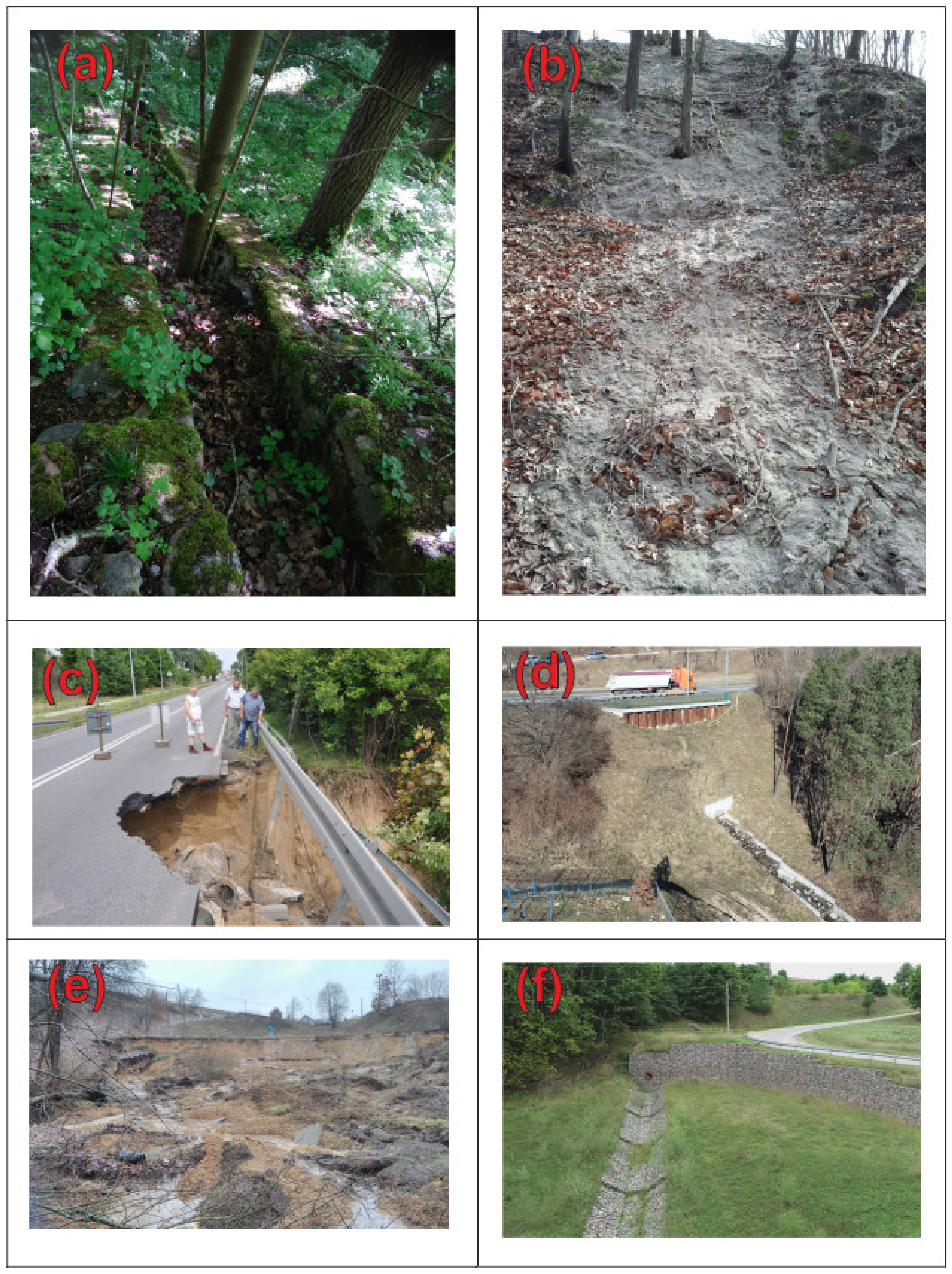
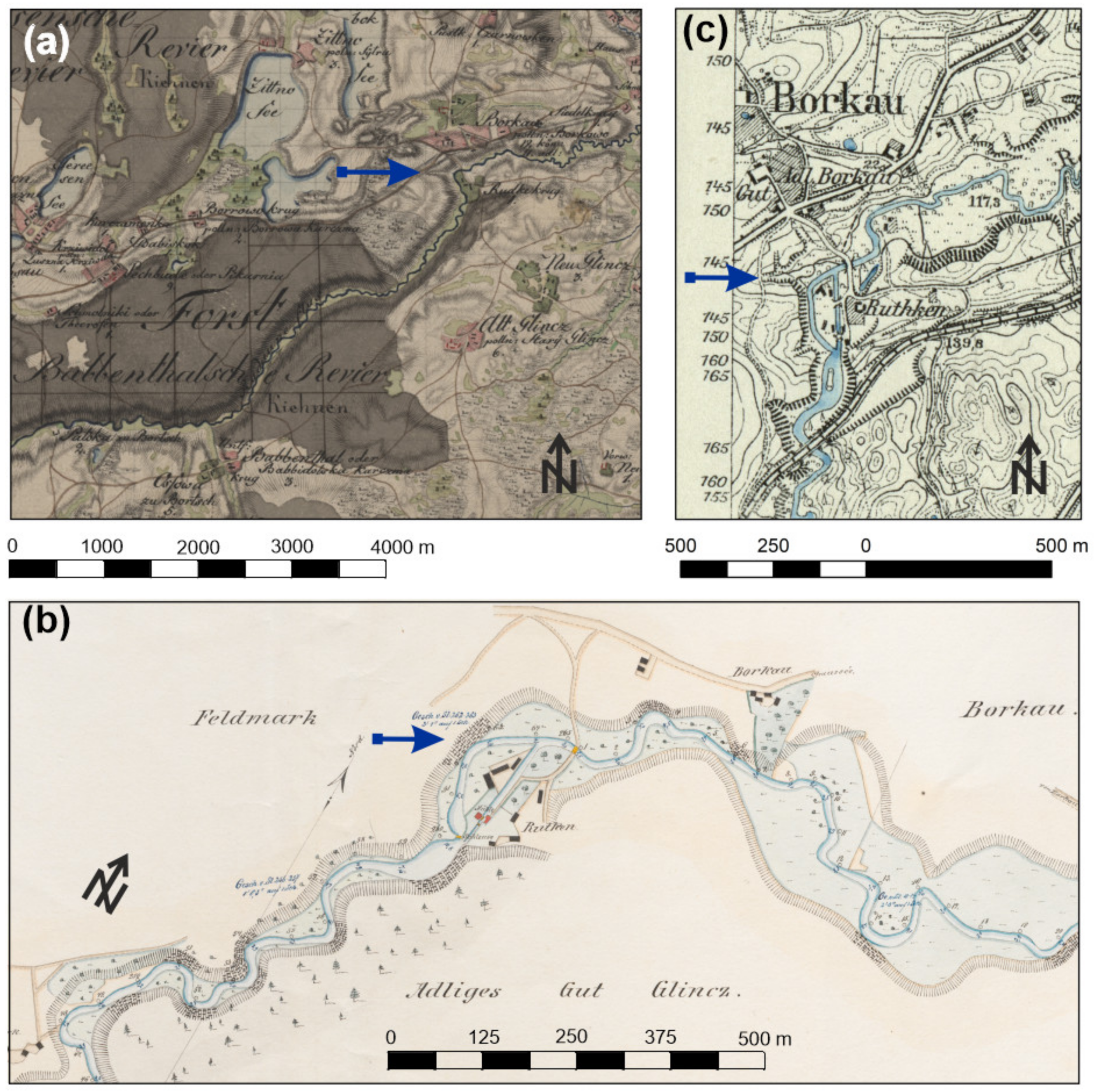
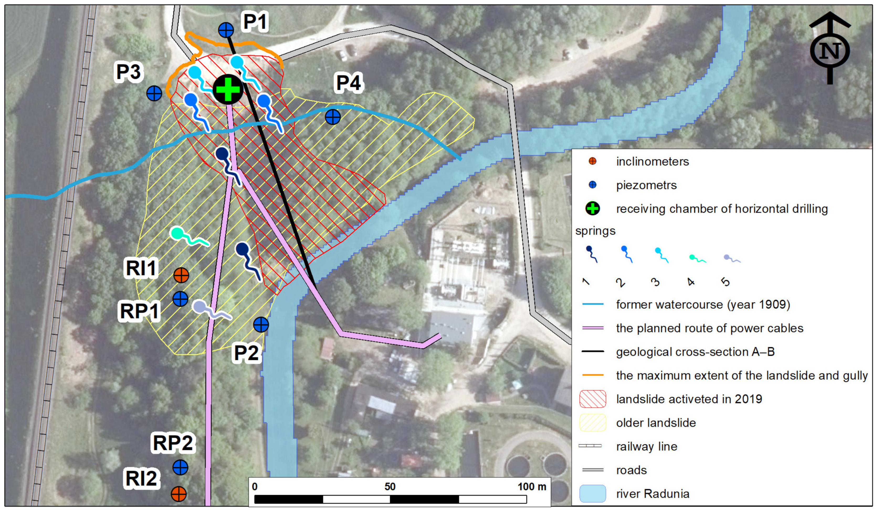
3.2. An Example of Anthropogenic Causes of the Rutki Landslide
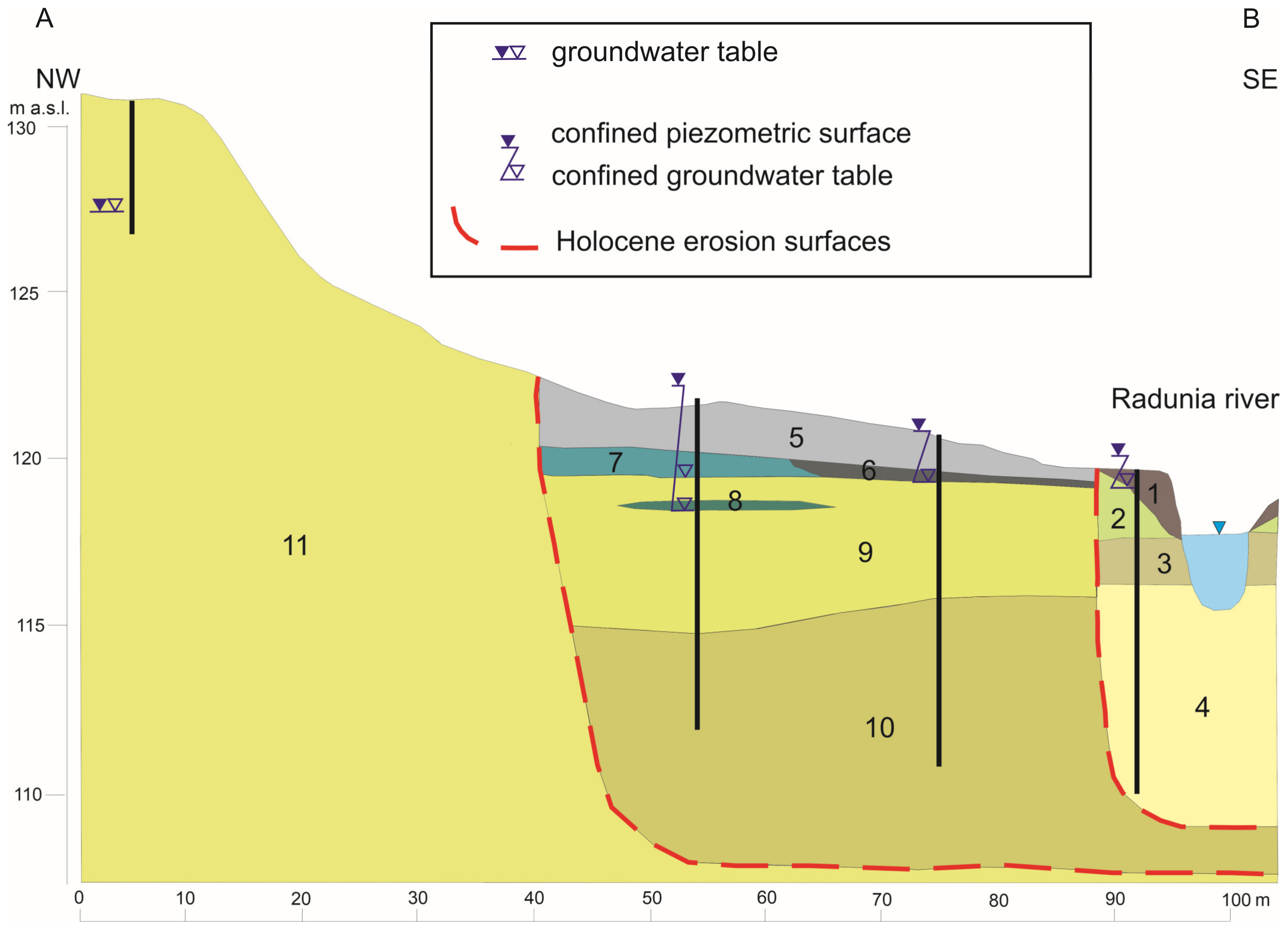
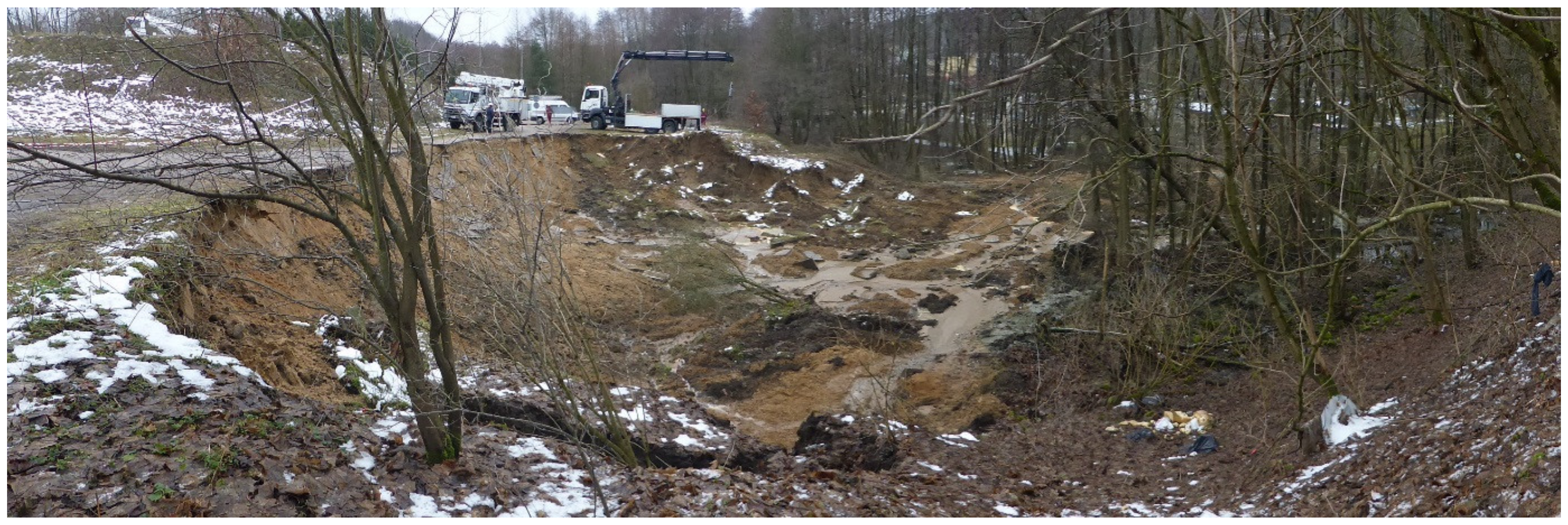
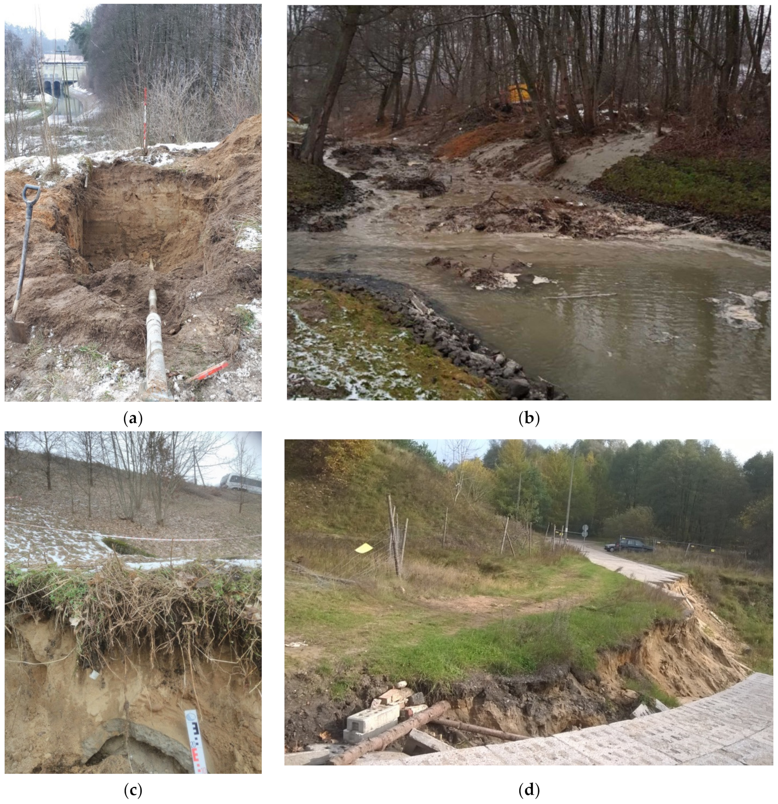
3.2.1. Description of the Landslide’s Development and Structure
3.2.2. Numerical Analysis of the Landslide’s Development
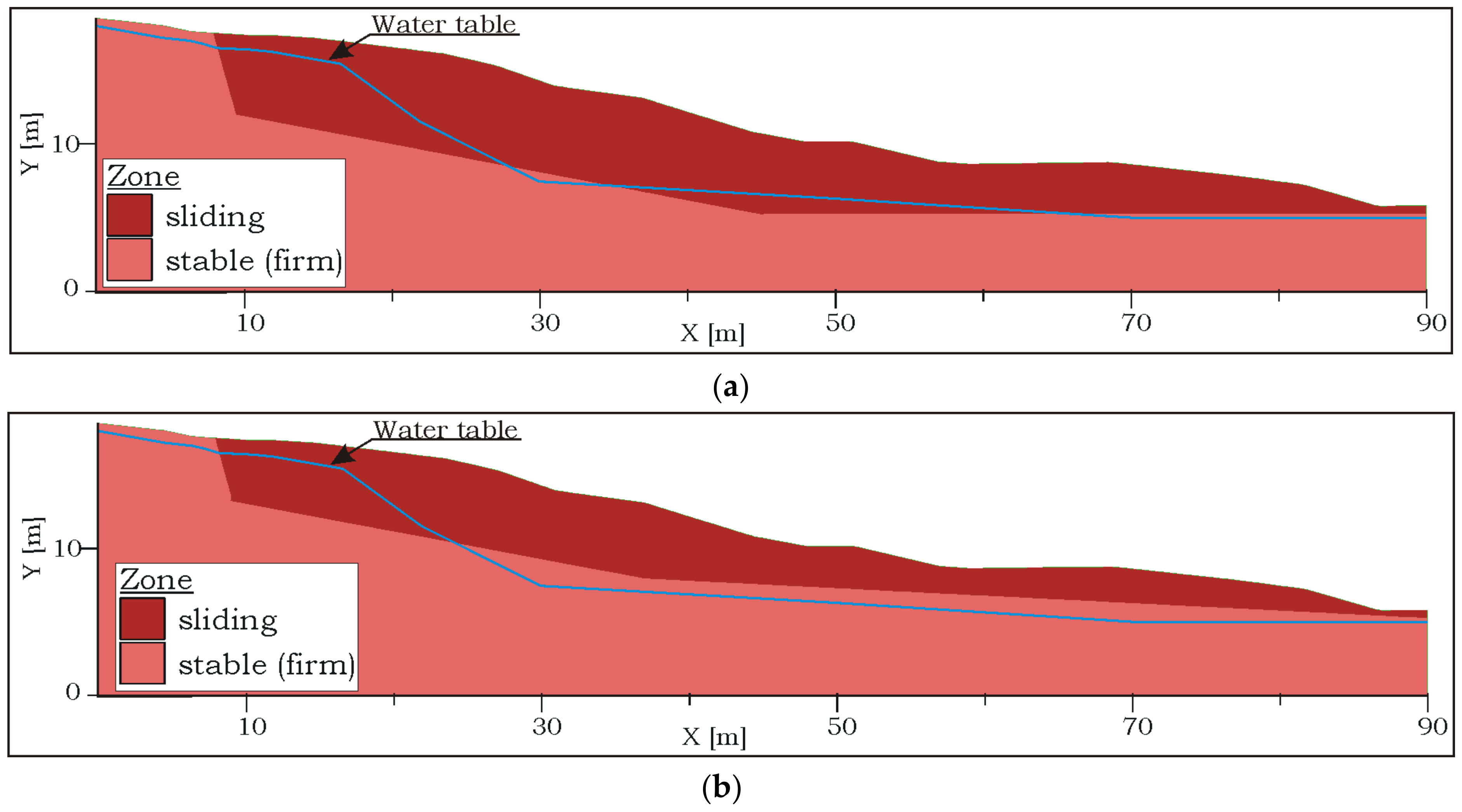
Elaboration of the Landslide Model
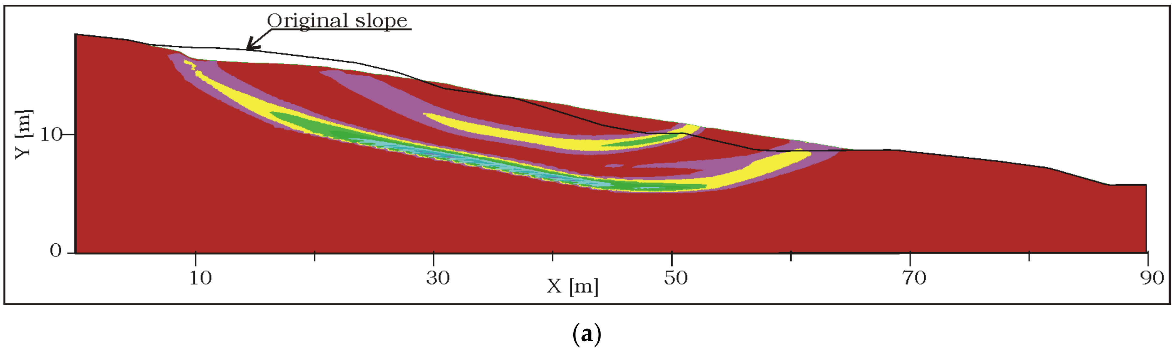
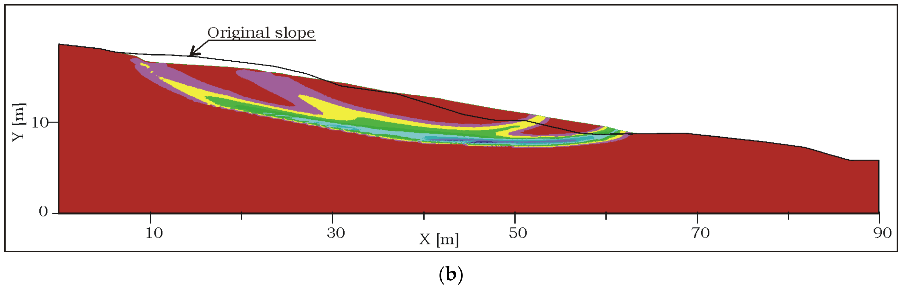
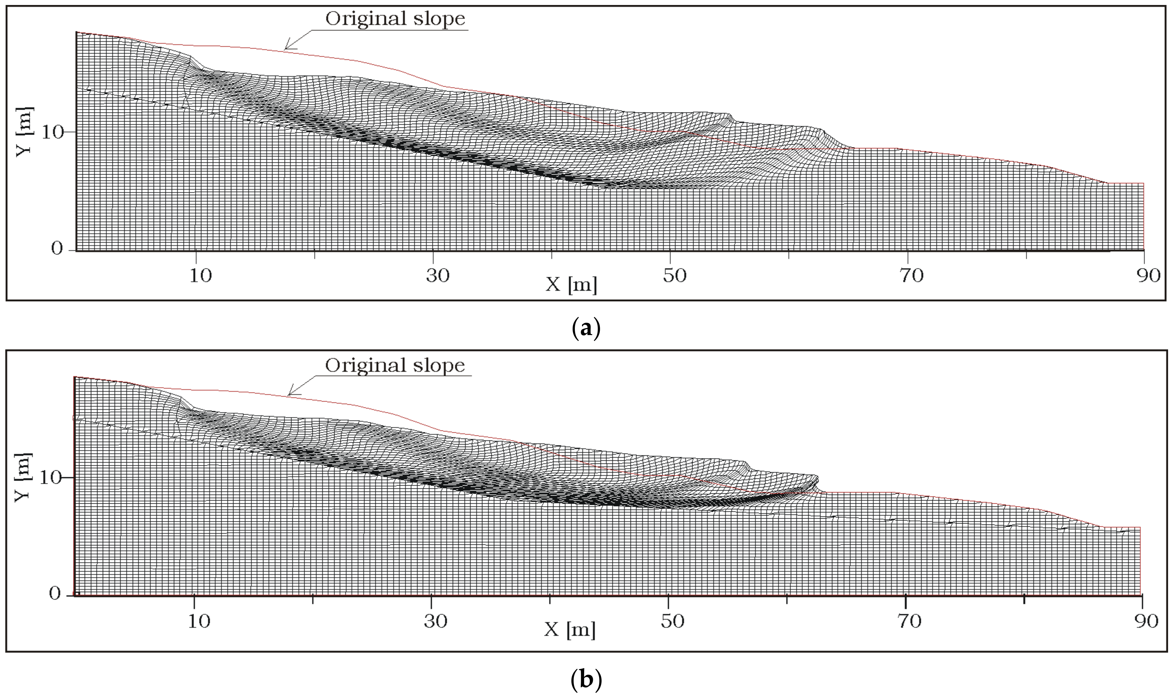
Results of the Landslide Simulation
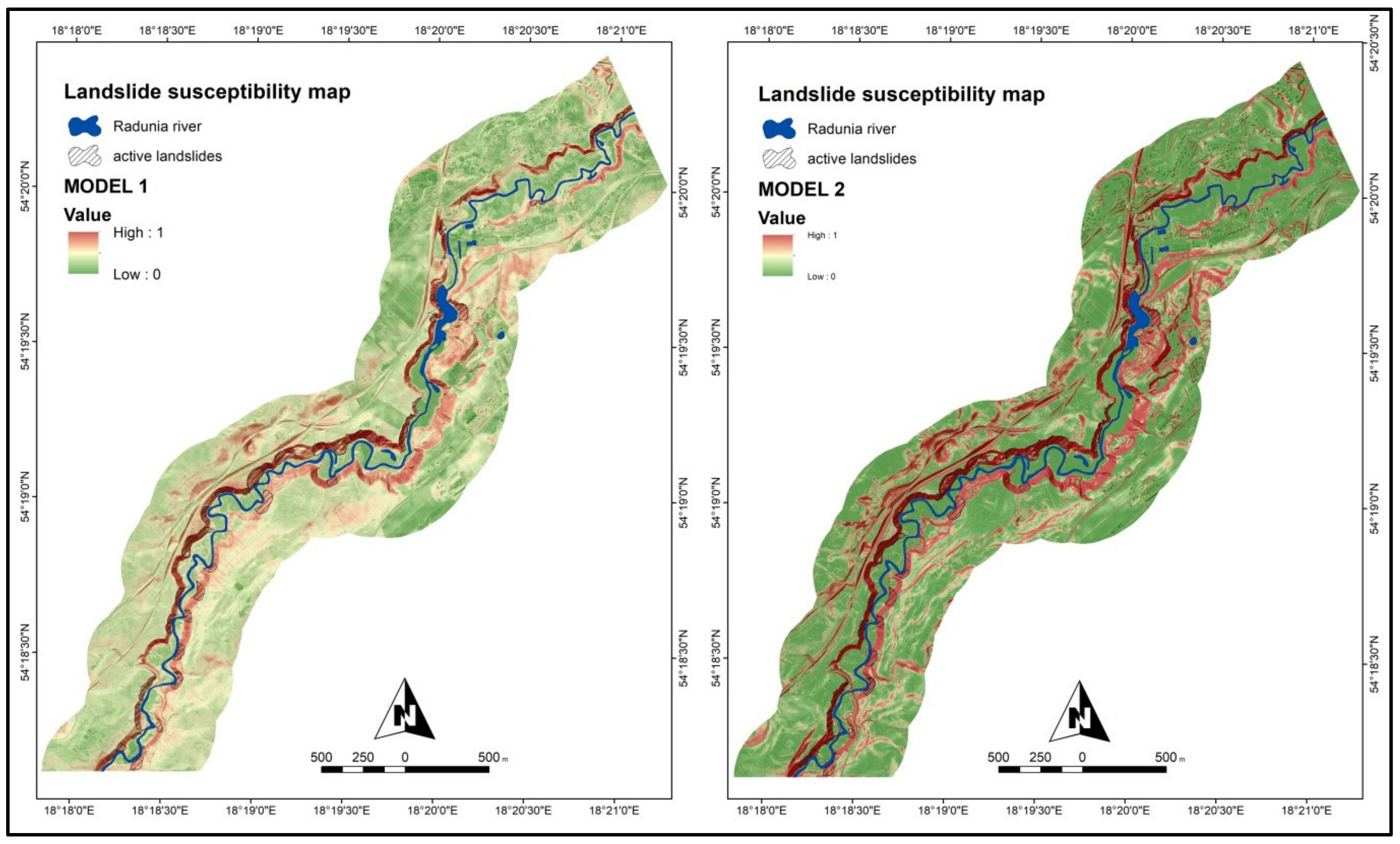
3.3. Landslide Susceptibility Map of Central Radunia Valley
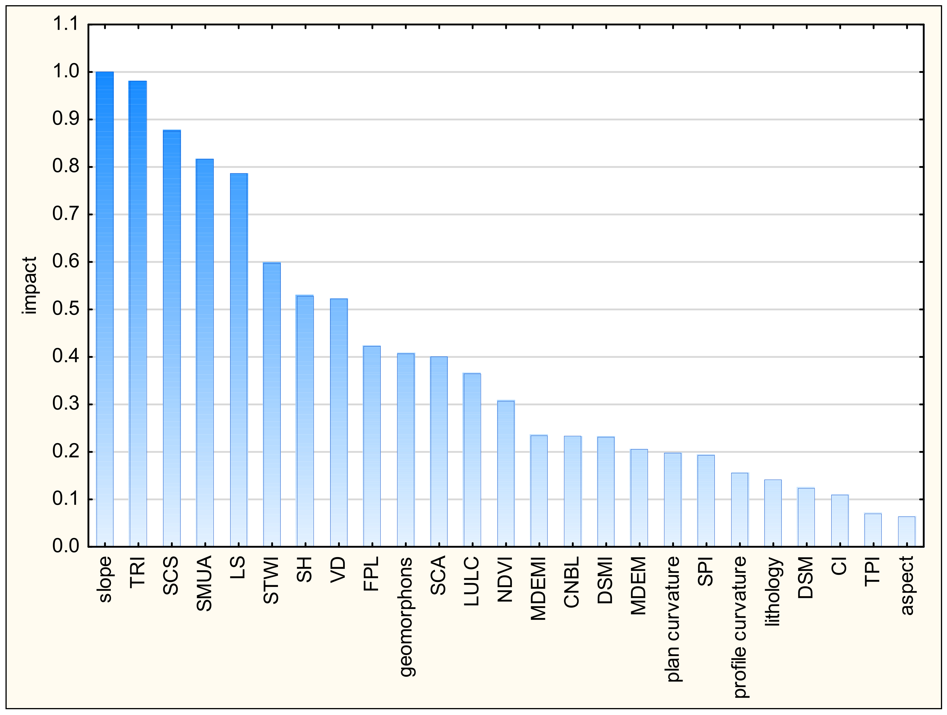
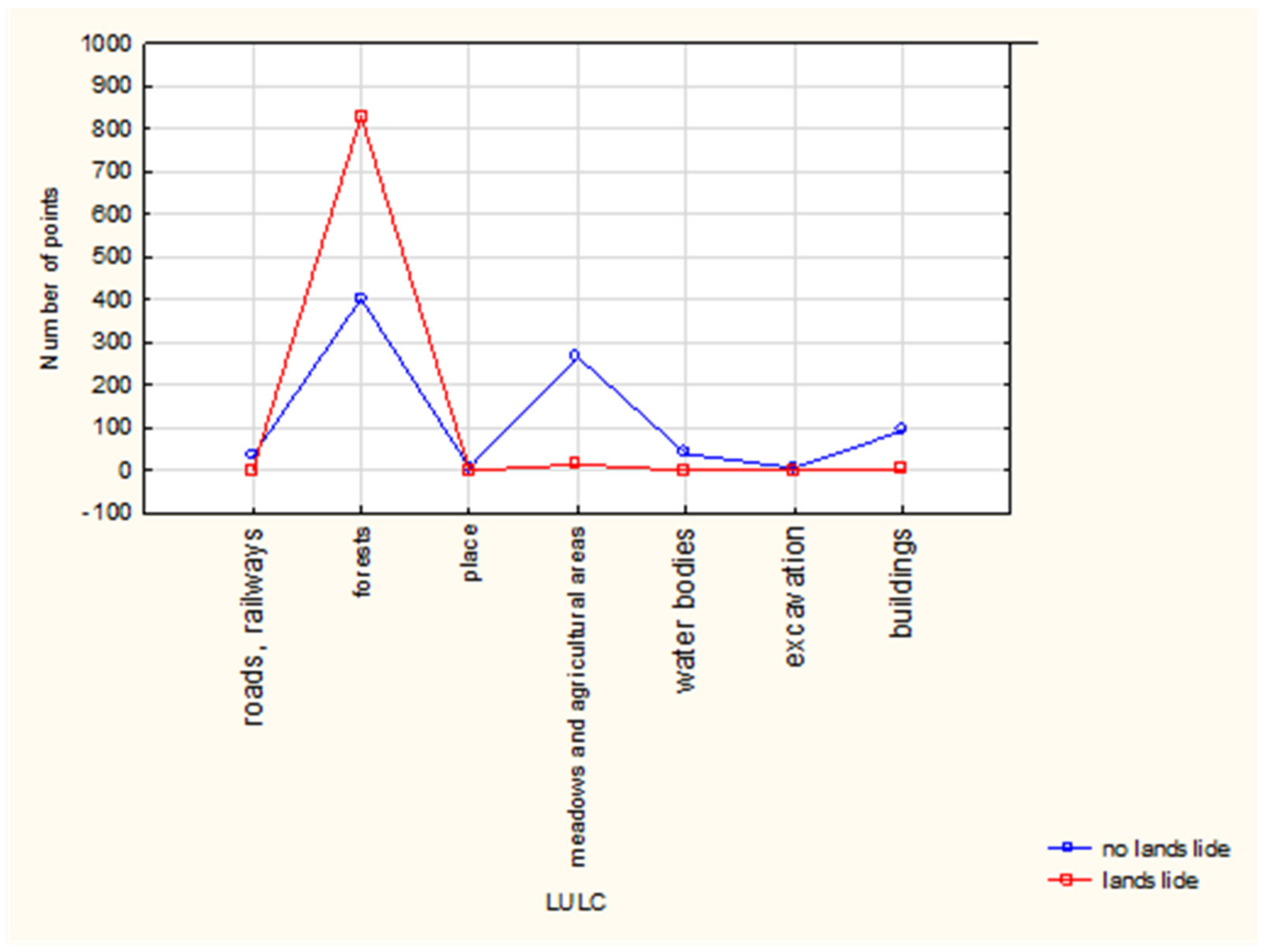
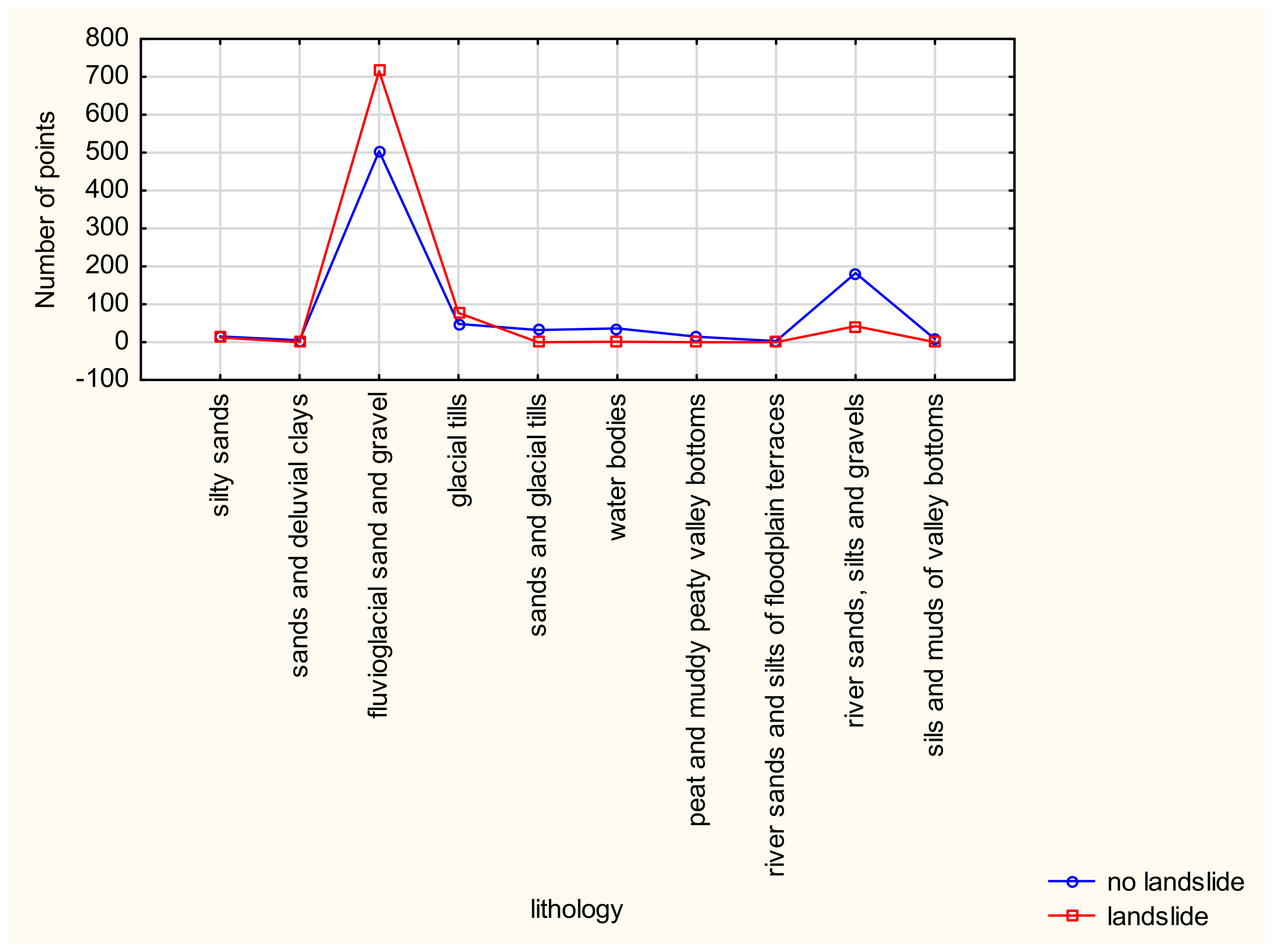
3.3.1. Relationship between Landslide and Conditioning Factors
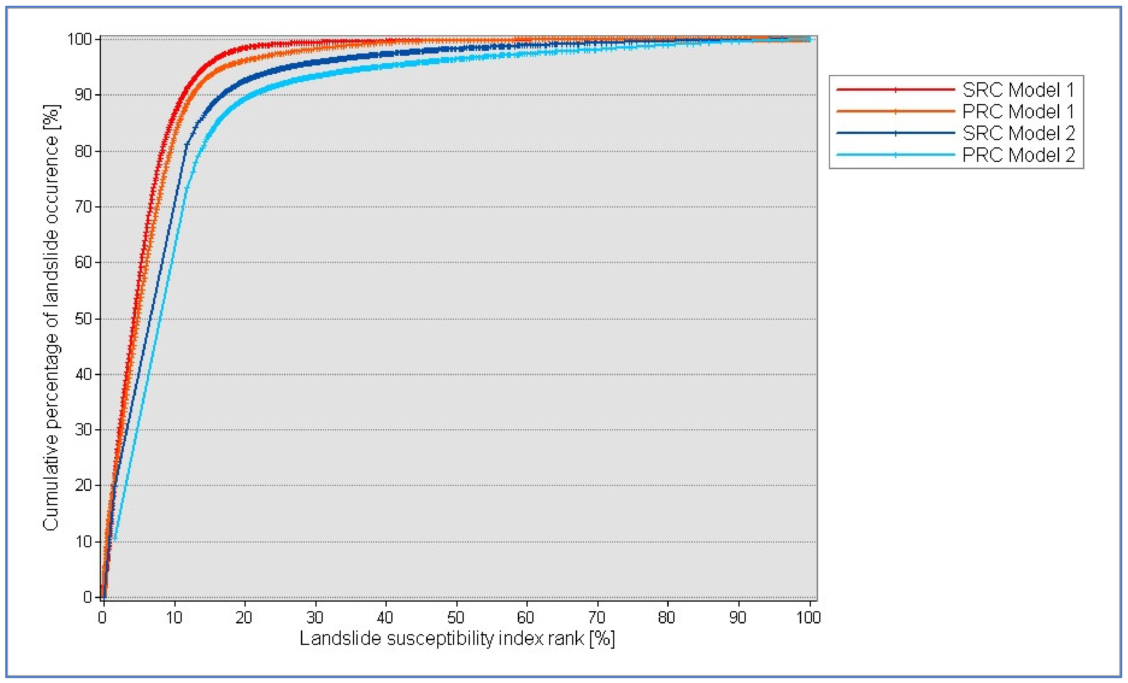
3.3.2. Logistic Regression Model
4. Discussion
4.1. Landslide-Triggering Factors
4.2. The Role of Causal Factors in the Formation of Landslides
4.3. The Roles of High-Resolution DEMs and Modified DEMs in Susceptibility Assessment
5. Conclusions
Author Contributions
Funding
Data Availability Statement
Acknowledgments
Conflicts of Interest
References
- Ostoja-Zagórski, J. Najstarsze Dzieje Ziem Polskich; Wydawnictwo Uniwersytetu Kazimierza Wielkiego w Bydgoszczy: Bydgoszcz, Poland, 2005; p. 252. [Google Scholar]
- Thiel, K. Kształtowanie Fliszowych Stoków Karpackich Przez Ruchy Masowe—Na Przykładzie Badań Na Stoku Bystrzyca w Szymbarku; Prace Instytutu Budownictwa Wodnego PAN: Gdańsk/Kraków, Poland, 1989; Volume 17, p. 91. [Google Scholar]
- Gil, E. Meteorological and hydrological conditions of landslides, Polish Flysch Carpathians. Stud. Geomorphol. Carpath-Balc. 1997, 31, 143–158. [Google Scholar]
- Glade, T. Modelling landslide triggering rainfall thresholds at a range of complexities—Landslides in Research, Theory and Practice. In Proceedings of the 8th International Symposium on Landslides, Cardiff, UK, 26–30 June 2000; Bromhead, E., Ed.; pp. 633–640. [Google Scholar]
- Gil, E.; Zabuski, L.; Mrozek, T. Hydrometeorological conditions and their relation to landslide processes in the Polish Flysch Carpathians (an example of Szymbark area). Stud. Geomorphol. Carpatho-Balc. 2009, 43, 127–143. [Google Scholar]
- Tyszkowski, S. Badania rozwoju osuwisk w rejonie Świecia, na podstawie materiałów fotogrametrycznych. Landf. Anal. 2008, 9, 385–389. (In Polish) [Google Scholar]
- Tyszkowski, S. Distribution and origin of contemporary lowland landslides in the area of the direct river impact, on the example of section of Lower Vistula Valley between Morsk and Wiąg. Landf. Anal. 2014, 25, 159–167, (In Polish with English Summary). [Google Scholar] [CrossRef]
- Lévy, S.; Jaboyedoff, M.; Locat, J.; Demers, D. Erosion and channel change as factors of landslides and valley formation in Champlain Sea Clays: The Chacoura River, Quebec, Canada. Geomorphology 2012, 145–146, 12–18. [Google Scholar] [CrossRef]
- Yenes, M.; Monterrubio, S.; Nespereira, J.; Santos, G.; Fernández-Macarro, B. Large landslides induced by fluvial incision in the Cenozoic Duero Basin (Spain). Geomorphology 2015, 246, 263–276. [Google Scholar] [CrossRef]
- Kaczmarek, H.; Tyszkowski, S.; Banach, M. Landslide development at the shores of a dam reservoir (Włocławek, Poland), based on 40 years of research. Environ. Earth Sci. 2015, 74, 4247–4259. [Google Scholar] [CrossRef]
- Korup, O. Landslide dam. In Encyclopedia of Geomorphology; Goudie, A., Ed.; Routlege: London, UK, 2004; 1156p. [Google Scholar]
- Korup, O. Large landslides and their effect on sediment flux in South Westland, New Zealand. Earth Surf. Process. Landf. 2005, 30, 305–323. [Google Scholar] [CrossRef]
- Glenn, N.F.; Streutker, D.R.; Chadwick, D.J.; Thackray, G.D.; Dorsch, S.J. Analysis of LiDAR-derived topographic information for characterizing and differentiating land-slide morphology and activity. Geomorphology 2006, 73, 131–148. [Google Scholar] [CrossRef]
- Fuller, I.C.; Riedler, R.A.; Bell, R.; Marden, M.; Glade, T. Landslide-driven erosion and slope–channel coupling in steep, forested terrain, Ruahine Ranges, New Zealand, 1946–2011. Catena 2016, 142, 252–268. [Google Scholar] [CrossRef]
- Alonso, E.E.; Pinyol, N.M.; Puzrin, A.M. Catastrophic Slide: Vaiont Landslide, Italy; Alonso, E.E., Pinyol, N.M., Puzrin, A.M., Eds.; Geomechanics of Failures; Advanced Topics; Springer: Dordrecht, The Netherlands; Heidelberg, Germany; London, UK; New York, NY, USA, 2010; pp. 33–81. [Google Scholar]
- Wolter, A.; Stead, D.; Ward, B.C.; Clague, J.J.; Ghirotti, M. Engineering geomorphological characterisation of the Vajont Slide, Italy, and a new interpretation of the chronology and evolution of the landslide. Landslides 2015, 13, 1067–1081. [Google Scholar] [CrossRef]
- Guzzetti, F.; Reichenbach, P.; Cardinali, M.; Galli, M.; Ardizzone, F. Probabilistic landslide hazard assessment at the basin scale. Geomorphology 2005, 72, 272–299. [Google Scholar] [CrossRef]
- Pourghasemi, H.R.; Pradhan, B.; Gokceoglu, C.; Mohammadi, M.; Moradi, H.R. Application of weights-ofevidence and certainty factor models and their comparison in landslide susceptibility mapping at Haraz watershed, Iran. Arab. J. Geosci. 2013, 6, 2351–2365. [Google Scholar] [CrossRef]
- Reichenbach, P.; Rossi, M.; Malamud, B.; Mihir, M.; Guzzetti, F. A review of statistically-based landslide susceptibility models. Earth-Sci. Rev. 2018, 180, 60–91. [Google Scholar] [CrossRef]
- Małka, A. Landslide susceptibility mapping of Gdynia using geographic information system-based statistical models. Nat. Hazards 2021, 107, 639–674. [Google Scholar] [CrossRef]
- Banach, M.; Kaczmarek, H.; Tyszkowski, S. Development of landslides in shore zones of water reservoir on an example of the central landslide at Dobrzyń on the Vistula, Włocławek Reservoir. Przegląd Geogr. 2013, 85, 397–415. (In Polish) [Google Scholar] [CrossRef]
- Bernardie, S.; Desramaut, N.; Malet, J.-P.; Gourlay, M.; Grandjean, G. Prediction of changes in landslide rates induced by rainfall. Landslides 2015, 12, 481–494. [Google Scholar] [CrossRef]
- Vassallo, R.; Grimaldi, G.M.; Di Malo, C. Pore pressures induced by historical rain series in a clay landslide: 3D modelling. Landslides 2015, 12, 731–744. [Google Scholar] [CrossRef]
- Zabuski, L.; Kulczykowski, M. Współczesne procesy osuwiskowe na klifie w Jastrzębiej Górze. Przegląd Geol. 2020, 68, 682–690. Available online: https://www.pgi.gov.pl (accessed on 8 January 2022).
- Zabuski, L.; Kulczykowski, M.; Świdziński, W. Identification of the Causes of a Landslide in Koronowo (Polish Lowlands). AHEM 2019, 66, 47–56. [Google Scholar] [CrossRef]
- Marks, L. Timing of the late Vistulian (wechselian) glacial phases in Poland. Quat. Sci. Rev. 2012, 44, 81–88. [Google Scholar] [CrossRef]
- Rachocki, T. Przebieg i natężenie współczesnych procesów rzecznych w korycie Raduni. Dok. Geogr. 1974, 4, 7–121. [Google Scholar]
- Piasecki, D. Szkic geologiczno-morfologiczny dorzecza Raduni. Rocz. Pol. Tow. Geol. 1960, 4, 385–390. [Google Scholar]
- Woś, A. Klimat Polski; Wydawn Naukowe PWN: Warszawa, Poland, 1999. [Google Scholar]
- Licbarski, P. Komentarz do Mapy Hydrograficznej Polski w Skali 1:50,000, Arkusz 325.1 Pruszcz Gdański; GUGiK: Warszawa, Poland, 1989. [Google Scholar]
- Jereczek-Korzeniewska, K. Komentarz do Mapy Hydrograficznej Polski w Skali 1:50,000, Arkusz N-34-49-D Gdańsk-Osowa; GUGiK: Warszawa, Poland, 2005. [Google Scholar]
- Owaczarek, M.; Filipiak, J. Contemporary changes of thermal conditions in. 2016. Poland, 1951–2015. Bull. Geography. Phys. Geogr. Ser. 2016, 10, 31–50. [Google Scholar] [CrossRef]
- Petelski, K.; Staszek, W. The Detailed Geological Map of Poland in Scale 1:50,000. Rumia 15. PGI–NRI. 2001. Available online: http://baza.pgi.gov.pl (accessed on 8 January 2022). (In Polish)
- Pikies, R. The Detailed Geological Map of Poland in Scale 1:50,000. Żukowo 26. PGI–NRI. 2001. Available online: http://baza.pgi.gov.pl (accessed on 8 January 2022). (In Polish)
- Koutaniemi, L.; Rachocki, A. Palaeohydrology and landscape development in the middle course of the Radunia basin, North Poland. Fenn. Int. J. Geogr. 1981, 159, 335–342. [Google Scholar]
- Błaszkiewicz, M.; Piotrowski, J.A.; Brauer, A.; Gierszewski, P.; Kordowski, J.; Kramkowski, M.; Lamparski, P.; Lorenz, S.; Noryśkiewicz, A.M.; Ott, F.; et al. Climatic and morphological controls on diachronous postglacial lake and river valley evolution in the area of Last Glaciation, northern Poland. Quat. Sci. Rev. 2015, 109, 13–27. [Google Scholar] [CrossRef]
- Kühn, B. Geologische Spezialkarte von Preußen und den Thüringischen Staaten. Maßstab 1:25,000; Zuckau, B., Ed.; Königlich Preussische Geologische Landesanstalt/Staatsbiliothek: Berlin, Germany, 1905. [Google Scholar]
- Blockus, M. Ekspertyza Techniczna Dotycząca Osuwiska w Rejonie Miejscowości Rutki w Powiecie Kartuskim, w Gminie Żukowo nad Radunią, Woj; Pomor: Gdańsk, Poland, 2019. [Google Scholar]
- Lidzbarski, M.; Potrykus, D.; Tarnawska, E.; Szelewicka, A.; Pasierowska, B.; Kowalewski, T. Studium Możliwości Weryfikacji Istniejącej strefy Ochronnej Ujęcia Wody “Straszyn”; PGI–NRI: Warszawa, Poland, 2019. [Google Scholar]
- Świstulski, D. Zabytkowe obiekty o tematyce elektrotechnicznej w województwie pomorskim. Zesz. Nauk. Wydziału Elektrotech. Autom. Politech. Gdańskiej 2013, 35, 45–49. [Google Scholar]
- Kulczykowski, M. Metoda gwoździowania w warunkach awarii konstrukcji oporowych. In Proceedings of the Wyd Konferencji Naukowo-Technicznej “Awarie Budowlane ‘96”, Szczecin, Poland, 22–25 May 1996; Volume 2, pp. 475–482. [Google Scholar]
- Kulczykowski, M.; Przewłócki, J.; Konarzewska, B. Application of soil nailing technique for protection and preservation historical buildings. IOP Conf. Ser. Mater. Sci. Eng. 2017, 245, 022055. [Google Scholar] [CrossRef]
- Jereczek, K.; Rolka, A.M.; Szudarowski, W. Zbiornik Rutki jako basen sedymentacyjny. The Rutki reservoir as a depositional basin (in Polish with English summary). Przegląd Geogr. 1997, 69, 149–155. [Google Scholar]
- Karwik, A. Baza danych GIS Mapy Hydrogeologicznej Polski 1:50,000. Pierwszy Poziom Wodonośny, Występowanie i Hydrodynamika; PIG–PIB: Warszawa, Poland, 2006. Available online: https://geolog.pgi.gov.pl/ (accessed on 10 January 2023). (In Polish)
- Tarnawska, E. Baza danych GIS Mapy Hydrogeologicznej Polski 1:50,000. Pierwszy Poziom Wodonośny, Występowanie i Hydrodynamika. In Arkusz Dzierżążno; PGI–NRI: Warszawa, Poland; PIG–PIB: Warszawa, Poland, 2011; Volume 54. Available online: https://geolog.pgi.gov.pl/ (accessed on 8 January 2022). (In Polish)
- Staszek, W. Komentarz do Mapy Hydrograficznej Polski w Skali 1:50,000, Arkusz N-34-61-B Kolbudy Górne; GUGiK: Warszawa, Poland, 2005. [Google Scholar]
- Widernik, M. Magistrala węglowa Śląsk—Gdynia i jej znaczenie w okresie międzywojennym. Zap. Hist. 1984, 2, 31–52. [Google Scholar]
- Fałtynowicz, W.; Królak, D. Lichens of the nature reserve “Jar Rzeki Raduni” in the Kaszubskie Lake District (Northern Poland). Acta Bot. Cassubica 2001, 2, 133–141. [Google Scholar]
- Pawalczyk, P. Ochrona procesów generowanych przez rzeki jako podstawa ochrony przyrody w ich dolinach. Przegląd Przyr. VI 1995, 3, 235–255, (In Polish with English Summary). [Google Scholar]
- Schrötter, F.L. 1796–1802. Karte von Ost-Preussen nebst Preussisch Litthauen und West-Preussen nebst dem Netzdistrict aufgenommen unter Leitung des Königl. Preuss. Staats Ministers Frey Herrn von Schroetteer in den Jahren von 1796 bis 1802; Staatsbibliothek zu Berlin: Berlin, Germany, 1812. [Google Scholar]
- Strempel. Urmesstischblatt, Topographische Karte, Maßstab 1:25,000, Blatt Zuckau; Staatsbiliothek: Berlin, Germany, 1862. [Google Scholar]
- Breia, M. Situations Plan des Radyne Flusses Section III, von Babebthal bis Zuckau. Vermessen 1859 vom Feldmesser Buchwald, Gezeichnet 1860 vom Feldmesser Guth. Cpirt im Mai 1881 durch M. Breia Regierungs Geometer; Archiwum Państwowe w Gdańsku: Gdańsk, Poland, 1881. [Google Scholar]
- Messtischblatt. Topographische Karte, Maßstab 1:25,000, Blatt Zuckau; Staatsbiliothek: Berlin, Germany, 1900. [Google Scholar]
- Blockus, M.; Gast, M. Projekt Budowlany Prac Naprawczych w Rejonie Osuwiska Rutki w Gminie Żukowo nad Radunią na Działkach nr 85/1; 84/2; 85/1; 157/4; Gdańsk, Poland, 2019. [Google Scholar]
- Frydel, J.; Mil, L.; Szarafin, T.; Koszka-Maroń, D.; Przyłucka, M. Zmienność czasowa i zróżnicowanie przestrzenne wielkości i tempa erozji klifu Zatoki Usteckiej w rejonie Orzechowa. Landf. Anal. 2017, 34, 3–14. [Google Scholar] [CrossRef]
- Wódka, M. Conditions of landslide development during the last decade in the Rożnów Dam-Lake region (Southern Poland) based on Airborne Laser Scanning (ALS) data analysis. Geol. Q. 2022, 66, 66. [Google Scholar] [CrossRef]
- Itasca, C.G. FLAC 7.0 Manual; Minneapolis, MN, USA, 2011; Available online: https://docs.itascacg.com/flac3d700/flac3d/docproject/source/modeling/introduction/guidetohelp.html (accessed on 8 January 2022).
- Chung, C.F.; Fabbri, A.G. Validation of spatial prediction models for landslide hazard mapping. Nat. Hazards 2003, 30, 451–472. [Google Scholar] [CrossRef]
- Wang, Y.; Feng, L.; Li, S.; Ren, F.; Du, Q. A hybrid model considering spatial heterogeneity for landslide susceptibility mapping in Zhejiang Province, China. Catena 2020, 188, 104425. [Google Scholar] [CrossRef]
- Wiegand, T. Modellierung von Massenverlagerungen und ihre Darstellung in Gafahrungskarten auf Blatt 7719 Balingen mit Hilfe von Geoinformationssystemen (GIS). Angew. Geogr. Informationsverarbeitung VIII Salzburger Geogr. Mater. 1996, 24. [Google Scholar]
- Ayalew, L.; Yamagishi, H.; Marui, H.; Kanno, T. Landslides in Sado Island of Japan: Part II. GIS-based susceptibility mapping with comparisons of results from two methods and verifications. Eng. Geol. 2005, 81, 432–445. [Google Scholar] [CrossRef]
- Trigila, A.; Iadanza, C.; Esposito, C.; Scarascia-Mugnozza, G. Comparison of logistic regression and random forests techniques for shallow landslide susceptibility assessment in Giampilieri (NE Sicily, Italy). Geomorphology 2015, 249, 119–136. [Google Scholar] [CrossRef]
- Bai, S.; Lu, P.; Wang, J. Landslide susceptibility assessment of the Youfang catchment using logistic regression. J. Mt. Sci. 2015, 12, 816–827. [Google Scholar] [CrossRef]
- Lee, S.; Woo, J.; Kwan-Young, O.; Moung-Jin, L. The spatial prediction of landslide susceptibility applying artificial neural network and logistic regression models: A case study of Indie, Korea. Open Geosci. 2016, 8, 117–132. [Google Scholar] [CrossRef]
- Hemasinghe, H.; Rangali, R.S.S.; Deshapriya, N.L.; Samarakoon, L. Landslide susceptibility mapping using logistic regression model (a case study in Badulla District, Sri Lanka). Procedia Eng. 2018, 212, 1046–1053. [Google Scholar] [CrossRef]
- Lee, S. Application of likelihood ratio and logistic regression models to landslide susceptibility mapping using GIS. Environ. Manag. 2004, 34, 223–232. [Google Scholar] [CrossRef] [PubMed]
- Rasyid, A.R.; Bhandary, N.P.; Yatabe, R. Performance of frequency ratio and logistic regression model in creating GIS based landslides susceptibility map at Lompobattang Mountain, Indonesia. Geoenviron. Disasters 2016, 3, 19. [Google Scholar] [CrossRef]
- Oh, H.-J.; Kadavi, P.R.; Lee, C.-W.; Lee, S. Evaluation of landslide susceptibility mapping by evidential belief function, logistic regression and support vector machine models. Geomat. Nat. Hazards Risk 2018, 9, 1053–1070. [Google Scholar] [CrossRef]
- Małka, A. GIS-Based Landslide Susceptibility Modelling in Urbanized Areas: A Case Study of the Tri-City Area of Poland. GeoHazards 2022, 3, 508–528. [Google Scholar] [CrossRef]
- Hilbe, J.M. Logistic Regression Models; Chapman and Hall/CRC Press: New York, NY, USA, 2009. [Google Scholar]
- Bui, D.T.; Lofman, O.; Revhaug, I.; Dick, O. Landslide susceptibility analysis in the Hoa Binh province of Vietnam using statistical index and logistic regression. Nat. Hazards 2011, 59, 1413–1444. [Google Scholar] [CrossRef]
- Zêzere, J.L.; Pereira, S.; Melo, R.; Oliveira, S.C.; Garcia, R.A.C. Mapping landslide susceptibility using data-driven methods. Sci. Total Environ. 2017, 589, 250–267. [Google Scholar] [CrossRef]
- Pamela; Sadisun, I.A.; Arifianti, Y. Weights of evidence method for landslide susceptibility mapping in Takengon, Central Aceh, Indonesia. IOP Conf. Ser. Earth Environ. Sci. 2018, 118, 012037. [Google Scholar] [CrossRef]
- Varnes, D.J. Slope movement types and processes. In Landslides, Analysis and Control; Schuster, R.L., Krizek, R.J., Eds.; Special report 176: Transportation research board; National Academy of Sciences: Washington, DC, USA, 1978; pp. 11–33. [Google Scholar]
- Cruden, D.M.; Couture, R. The working classification of landslides: Material matters. In Proceedings of the 64th and 14th Pan-American conference on soil mechanics and geotechnical engineering, Toronto, ON, Canada, 2–6 October 2011; Available online: http://geoserver.ing.puc.cl/info/conferences/ (accessed on 8 January 2020).
- Hungr, O.; Leroueil, S.; Picarelli, L. The Varnes classification of landslide types, an update. Landslides 2014, 11, 167–194. [Google Scholar] [CrossRef]
- Dikau, R.; Brunsden, D.; Schrott, L.; Ibsen, M.L. Landslide Recognition. In Identification, Movement and Causes; International Association of Geomorphologists; John Wiley and Sons: Chichester, UK, 1996. [Google Scholar]
- Swets, J.A. Measuring the accuracy of diagnostic systems. Science 1988, 240, 1285–1293. [Google Scholar] [CrossRef] [PubMed]
- Mrozek, T.; Laskowicz, I.; Zabuski, L.; Kulczykowski, M.; Świdziński, W. Landslide susceptibility and risk assessment in a non-mountainous region—A case study of Koronowo, Northern Poland. Geol. Q. 2016, 60, 758–769. [Google Scholar] [CrossRef]
- Małka, A. Podatność i ryzyko osuwiskowe w obszarach rzeźby młodoglacjalnej, przeobrażonej antropogenicznie, na terenie Gdyni. Pr. doktorska. Arch. Państw. Inst. Geol. PIB 2018. [Google Scholar] [CrossRef]
- Starkel, L. Złożoność czasowa i przestrzenna opadów ekstremalnychich efekty geomorfologiczne i drogi przeciwdziałania im. Landf. Anal. 2011, 15, 65–80. [Google Scholar]
- Ossowski, P. Odprowadzanie Wód Opadowych od Istniejącego Przepustu Zlokalizowanego w Ciągu Drogi Wojewódzkiej nr 211 w m. Borkowo Dz 74/1 Obręb 0003 Borkowo; Zarząd Dróg Wojewódzkich w Gdańsku: Gdańsk, Poland, 2015. [Google Scholar]
- Segoni, S.; Tofani, V.; Rosi, A.; Catani, F.; Casagli, N. Combination of Rainfall Thresholds and Susceptibility Maps for Dynamic Landslide Hazard Assessment at Regional Scale. Front. Earth Sci. 2018, 6, 85. [Google Scholar] [CrossRef]
- Mondini, A.C.; Guzzetti, F.; Chang, K.-T.; Monserrat, O.; Martha, T.R.; Manconi, A. Landslide failures detection and mapping using Synthetic Aperture Radar: Past, present and future. Earth-Sci. Rev. 2021, 216, 103574. [Google Scholar] [CrossRef]
- Jakob, M. The impacts of logging on landslide activity at Clayoquot Sound, British Columbia. CATENA 2000, 38, 279–300. [Google Scholar] [CrossRef]
- Cannon, S.H.; Gartner, J.E. Wildfire-related debris flow from a hazards perspective. In Debris-Flow Hazards and Related Phenomena; Springer Praxis Books; Springer: Berlin/Heidelberg, Germany, 2005; pp. 363–385. [Google Scholar]
- Małka, A. Landslide susceptibility modelling using the index method and high-resolution airborne laser scanning data (LIDAR) in the area of Gdańsk. Przegląd Geol. 2015, 63, 301–311. Available online: https://www.pgi.gov.pl (accessed on 8 January 2022). (In Polish with English Summary).
- Wysokiński, L. Osuwisko w Brzeźnie powstałe w wyniku prac geofizycznych. Przegląd Geol. 1979, 8, 444–446. [Google Scholar]
- Banach, M. Zmiany jeziora Brzeźno po katastrofie w 1976 roku. Słupskie Pr. Geogr. 2005, 2, 113–220. [Google Scholar]
- Jiao, J.J.; Wang, X.-S.; Nandy, S. Confined groundwater zone and slope instability in weathered igneous rocks in Hong Kong. Eng. Geol. 2005, 80, 71–92. [Google Scholar] [CrossRef]
- Montgomery, D.R.; Dietrich, W.E. Where do channels begin. Nature 1988, 336, 232–234. [Google Scholar] [CrossRef]
- Grabowska-Olszewska, B. An influence of swelling on microstructural changes of bentonites studied with ESEM. Przegląd Geol. 2001, 49, 299–302. Available online: https://www.pgi.gov.pl (accessed on 8 January 2022). (In Polish with English Summary).
- Grabowski, D.; Laskowicz, I.; Małka, A.; Rubinkiewicz, J. Geoenvironmental conditioning of landsliding in river valleys of lowland regions and its significance in landslide susceptibility assessment: A case study in the Lower Vistula Valley, Northern Poland. Geomorphology 2022, 419, 108490. [Google Scholar] [CrossRef]
- Vakhshoori, V.; Zare, M. Landslide susceptibility mapping by comparing weight of evidence, fuzzy logic, and frequency ratio methods Geomatics. Nat. Hazards Risk Vol. 2016, 7, 1731–1752. [Google Scholar] [CrossRef]
- Arabameri, A.; Saha, S.; Roy, J.; Chen, W.; Blaschke, T.; Bui, D.T. Landslide Susceptibility Evaluation and Management Using Different Machine Learning Methods in The Gallicash River Watershed, Iran. Remote Sens. 2020, 12, 475. [Google Scholar] [CrossRef]
- Pawluszek, K.; Borkowski, A. Impact of DEM-derived factors and analytical hierarchy process on landslide susceptibility mapping in the region of Roznow Lake, Poland. Nat. Hazards 2016, 86, 919–952. [Google Scholar] [CrossRef]
- Perkins, J.P.; Reid, M.E.; Schmidt, K.M. Control of landslide volume and hazard by glacial stratigraphic architecture, northwest Washington State, USA. Geology 2017, 45, 1139–1142. [Google Scholar] [CrossRef]
- Hjulstrom, F. Studies of the morphological activity of rivers as illustrated by the river Fyris. Bull. Geol. Inst. Upps. 1935, 25, 221–527. [Google Scholar]
- Persichillo, M.G.; Bordoni, M.; Meisina, C.; Bartelletti, C.; Barsanti, M.; Giannecchini, R.; D’Amato Avanzi, G.; Galanti, Y.; Cevasco, A.; Brandolini, P.; et al. Shallow landslides susceptibility assessment in different environments. Geomat. Nat. Hazards Risk 2017, 8, 748–771. [Google Scholar] [CrossRef]
- Remondo, J.; González, A.; De Terán, J.R.D.; Cendrero, A.; Fabbri, A.; Chung, F. Validation of landslide susceptibility maps; examples and applications from a case study in Northern Spain. Nat. Hazards 2003, 30, 437–449. [Google Scholar] [CrossRef]
- Xiao, T.; Yu, L.; Tian, W.; Zhou, C.; Wang, L. Reducing Local Correlations Among Causal Factor Classifications as a Strategy to Improve Landslide Susceptibility Mapping. Front. Earth Sci. 2021, 9, 781674. [Google Scholar] [CrossRef]
- Wilson, J.P.; Gallant, J.C. (Eds.) Terrain Analysis: Principles and Applications; John Wiley & Sons: New York, NY, USA, 2000; pp. 1–27. [Google Scholar]
- Vatcheva, K.P.; Lee, M.; McCormick, J.B.; Rahbar, M.H. Multicollinearity in Regression Analyses Conducted in Epidemiologic Studies. Epidemiology 2016, 6, 227. [Google Scholar] [CrossRef] [PubMed]
- Kutner, M.; Nachtsheim, C.; Neter, J. Applied Linear Statistical Models, 4th ed.; McGraw-Hill: New York, NY, USA; Irwin: Huntersville, NC, USA, 2004. [Google Scholar]
- Wojciechowski, T.; Borkowski, A.; Perski, Z.; Wójcik, A. Airborne laser scanning data in landslide studies atthe example of the Zbyszyce landslide (Outer Carpathians). Przegląd Geol. 2012, 60, 95–102. Available online: https://www.pgi.gov.pl (accessed on 8 January 2022). (In Polish with English Summary).
- Perski, Z.; Wojciechowski, T.; Wójcik, A.; Borkowski, A. Monitoring of landslide dynamics with LIDAR, SAR interferometry and photogrammetry. Case study of Kłodne landslide. Southern Poland. In Proceedings of the World Landslide Forum 3, Beijing, China, 2–6 June 2014. [Google Scholar]
- Wójcik, A.; Wojciechowski, T.; Wódka, M.; Kaczorowski, J.; Kamieniarz, S.; Sikora, R.; Kułak, M.; Karwacki, K.; Warmuz, B.; Perski, Z. Development of landslide research at the Polish Geological Institute. Przegląd Geol. 2020, 68, 356–363. Available online: https://www.pgi.gov.pl (accessed on 8 January 2022). (In Polish with English Summary).
- Canavesi, V.; Segoni, S.; Rosi, A.; Ting, X.; Nery, T.; Catani, F.; Casagli, N. Different Approaches to Use Morphometric Attributes in Landslide Susceptibility Mapping Based on Meso-Scale Spatial Units: A Case Study in Rio de Janeiro (Brazil). Remote Sens. 2020, 12, 1826. [Google Scholar] [CrossRef]
- Stanley, T.; Kirschbaum, D.B. A heuristic approach to global landslide susceptibility mapping. Nat. Hazards 2017, 87, 145–164. [Google Scholar] [CrossRef]
- Wilde, M.; Günther, A.; Reichenbach, P.; Male, J.; Hervás, J. Pan-European landslide susceptibility mapping: ELSUS Version 2. J. Maps 2018, 14, 97–104. [Google Scholar] [CrossRef]
- Wojciechowski, T. Podatność osuwiskowa Polski. Prz. Geol. 2019, 67, 320–325, (In Polish with English Summary). [Google Scholar] [CrossRef]
- van Westen, C.J.; Castellanos, E.; Kuriakose, S.L. Spatial data for landslide susceptibility, hazard, and vulnerability assessment: An overview. Eng. Geol. 2008, 102, 112–131. [Google Scholar] [CrossRef]
- Soeters, R.; Van Westen, C.J. Slope instability recognition, analysis and zonation. In Landslides, Investigation and Mitigation; Turner, A.K., Schuster, R.L., Eds.; Transportation Research Board, National Research Council, Special Report 247; National Academy Press: Washington, DC, USA, 1996; pp. 129–177. [Google Scholar]
- Polykretis, C.; Faka, A.; Chalkias, C. Exploring the Impact of Analysis Scale on Landslide Susceptibility Modeling: Empirical Assessment in Northern Peloponnese, Greece. Geosciences 2018, 8, 261. [Google Scholar] [CrossRef]
- Burdziej, J.; Kunz, M. Ocena wpływu rozdzielczości i metody pozyskiwania danych wysokościowych na dokładność numerycznych modeli terenu oraz modeli spadków i ekspozycji. Estimation of resolution influence and methods of acquiring high-altitude data on the accuracy of numericterrain models and models of slopes and aspects. Arch. Fotogram. Kartogr. Teledetekcji 2006, 16, 111–123, (In Polish with English Summary). [Google Scholar]
- Booth, D.B.; Jackson, C.R. Urbanization of aquatic systems: Degradation thresholds, stormwater detention, and the limits of mitigation. J. Am. Water Resour. Assoc. 1997, 33, 1077–1090. [Google Scholar] [CrossRef]
- Strohbach, M.W.; Döring, A.O.; Möck, M.; Sedrez, M.; Mumm, O.; Schneider, A.-K.; Weber, S.; Schröder, B. The “Hidden Urbanization”: Trends of Impervious Surface in Low-Density Housing Developments and Resulting Impacts on the Water Balance. Front. Environ. Sci. 2019, 7, 29. [Google Scholar] [CrossRef]


| Scientific Research Methods | |||||
|---|---|---|---|---|---|
| Analysis of Secondary Data * | Analysis of Primary Data | ||||
| Field Surveys | Drilling/ Inclinometers, Piezometers | Numerical Analyses | Spatial Analyses | ||
| Investigation of the Rutki landslide with a scale of 1:500 | X | X | X | X | X |
| Assessment of the landslide susceptibility of the Central Radunia Valley with a scale of 1:5000 | X | X | X | ||
| Digital Data | Source | Thematic Layers | Websites |
|---|---|---|---|
| DEM*, field surveys*, engineering documentation*, scientific publications*, Google Earth™ imagery*, interviews with residents* | Landslide inventory | https://www.pgi.gov.pl/gdansk/projekty-krajowe/osuwiska-doliny-raduni.html *; accessed on 10 January 2023 | |
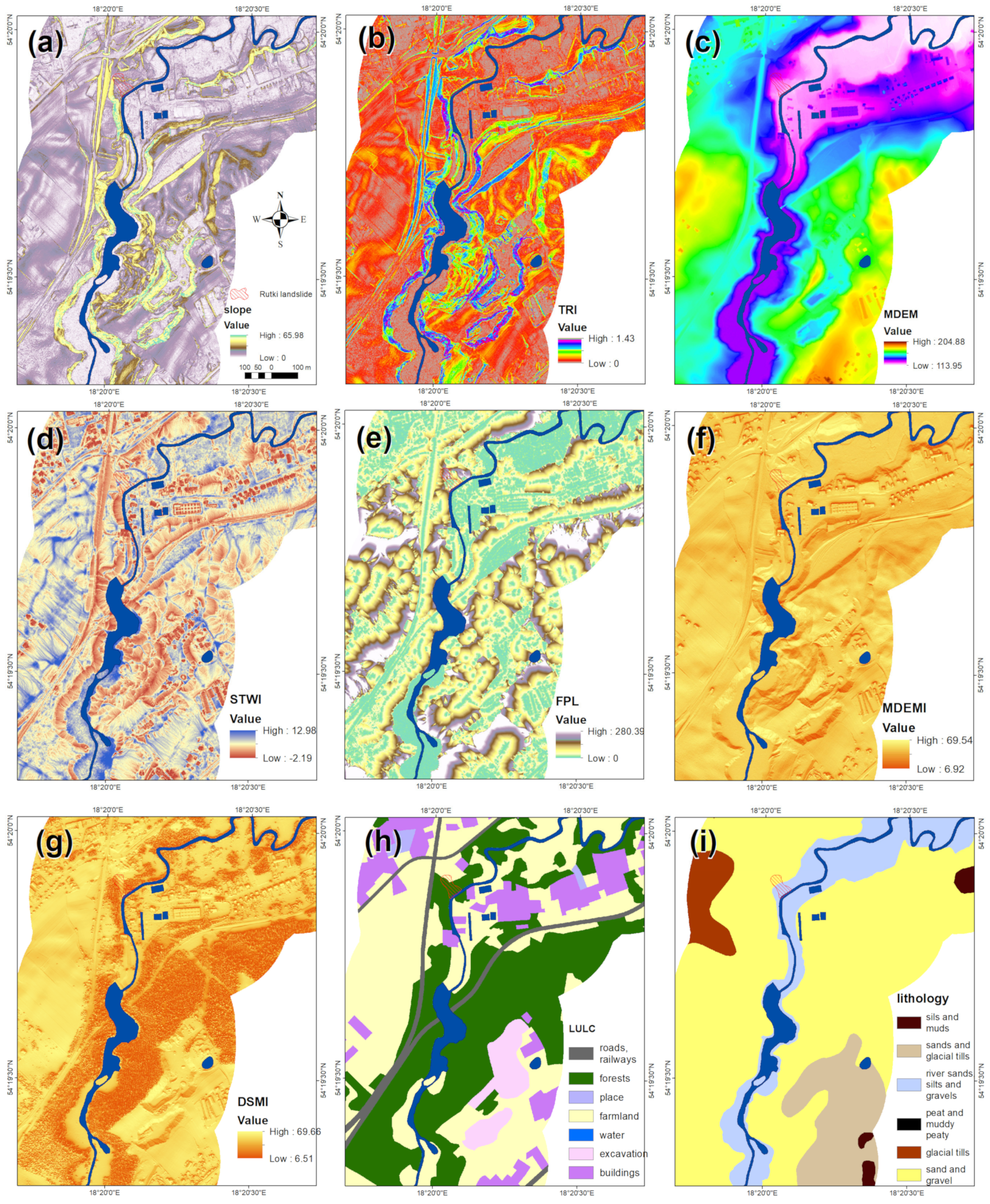
| Digital elevation model (DEM) | National Geodetic and Cartographic Resources, Poland | The topographic attributes: slope angle, slope height (SH), profile curvature, plan curvature, convergence index (CI), length slope factor (LS), topographic position index (TPI), valley depth (VD), slope mean of upslope area (SMUA), terrain ruggedness index (TRI), digital surface model (DSM), DSM insolation (DSMI), modified digital elevation model (MDEM), channel network base level (CNBL), SAGA catchment area (SCA), SAGA catchment slop (SCS), SAGA topographic wetness index (STWI), flow path length (FPL), stream power index (SPI), MDEM insolation (MDEMI), geomorphons, aspect | https://www.gov.pl/web/gugik; accessed on 10 January 2023 https://www.geoportal.gov.pl; accessed on 10 January 2023 https://www.pgi.gov.pl/gdansk/projekty-krajowe/osuwiska-doliny-raduni.html *; accessed on 10 January 2023 |
| Topographic object database (BDOT 10k) | National Geodetic and Cartographic Resources, Poland DEM*, field surveys* | Land use and land cover (LULC) | https://www.gov.pl/web/gugik; accessed on 10 January 2023 https://www.geoportal.gov.pl; accessed on 10 January 2023 https://www.pgi.gov.pl/gdansk/projekty-krajowe/osuwiska-doliny-raduni.html *; accessed on 10 January 2023 |
| Digital geological data | Polish Geological Institute, National Research Institute [33,34]; DEM*, field surveys* | Lithology | https://geologia.pgi.gov.pl; accessed on 10 January 2023 https://www.pgi.gov.pl/gdansk/projekty-krajowe/osuwiska-doliny-raduni.html *; accessed on 10 January 2023 |
| SENTINEL-2 satellite imagery | Sinergise Laboratory for geographical information systems Ltd., Slovenia | Normalised difference vegetation index (NDVI) | https://www.sentinel-hub.com https://www.pgi.gov.pl/gdansk/projekty-krajowe/osuwiska-doliny-raduni.html *; accessed on 10 January 2023 |
| No. | Dimensions | [m] | Measurement Type |
|---|---|---|---|
| 1 | Width of the displaced mass | 55 | Direct—measured on 13 January 2019 (field) |
| 2 | Length of the displaced mass | 85 | Direct—measured on 13 January 2019 (field) |
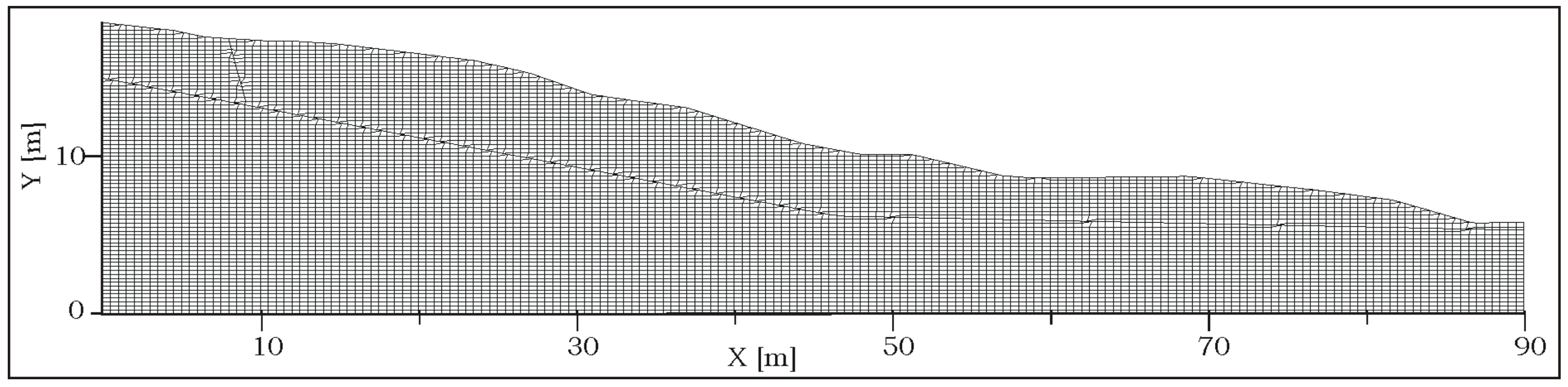
| 3 | Maximum depth of the displaced mass | 6 | Numerical model (Figure 13) |
| 4 | Height of the displaced mass | 4 | Direct—measured on 13 January 2019 (field) |
| 5 | Average depth of the failure surface | 2 | Numerical model (Figure 13) |
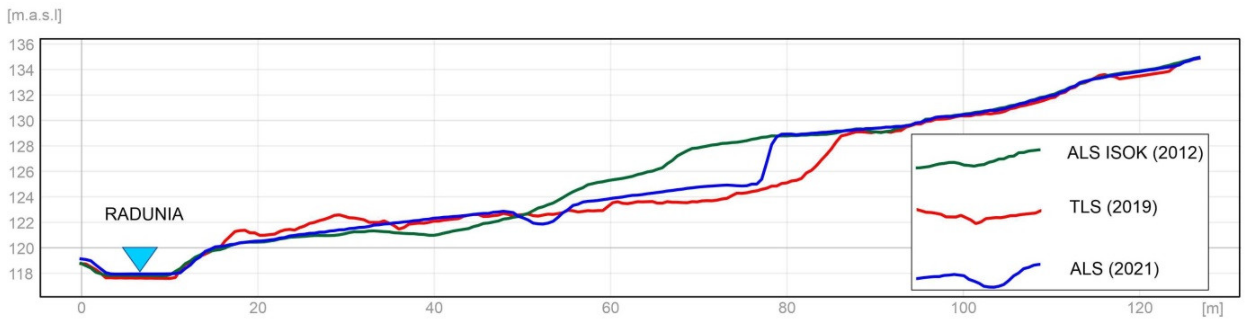
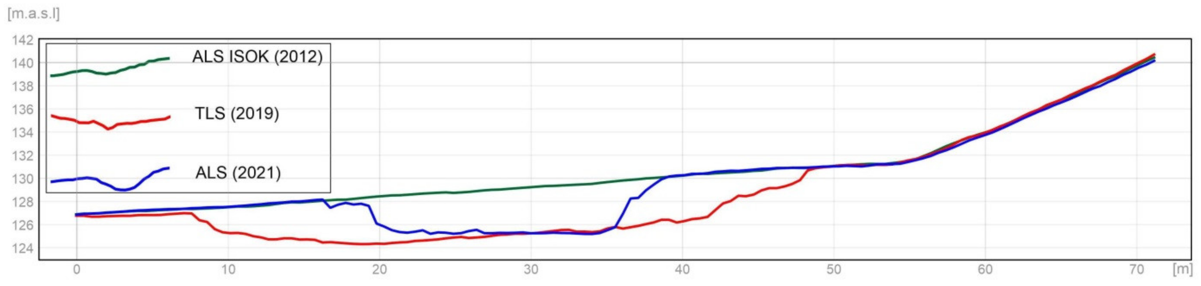
| 6 | Height of the main scarp | 4 | Topographic profiles (Figure 8 and Figure 9) |
| Model | AUC for SRC (%) | AUC for PRC (%) |
|---|---|---|
| Model 1 | 94.52 | 93.65 |
| Model 2 | 87.84 | 85.34 |
| Model 3 | 91.80 | 87.33 |
| Model 4 | 89.25 | 87.87 |
| Original Variable/Conditioning Factors | Factor Loadings (Varimax Normalised) Extract: Principal Components (the Marked Loadings Are > 0.7) | ||||
|---|---|---|---|---|---|
| Component 1 | Component 2 | Component 3 | Component 4 | Component 5 | |
| TRI | 0.88 * | −0.05 | 0.16 | 0.30 | −0.09 |
| SMUA | 0.87 | −0.12 | −0.15 | 0.14 | −0.04 |
| VD | 0.47 | −0.14 | −0.37 | 0.67 | −0.06 |
| TPI | −0.08 | 0.33 | 0.77 | −0.32 | 0.01 |
| LS | 0.40 | −0.03 | 0.28 | 0.54 | −0.16 |
| CI | −0.01 | 0.00 | 0.10 | 0.01 | 0.71 |
| profile curvature | −0.13 | 0.06 | 0.68 | −0.15 | 0.29 |
| plan curvature | 0.04 | −0.04 | 0.07 | −0.18 | 0.79 |
| slope | 0.89 | −0.05 | 0.16 | 0.31 | −0.09 |
| SH | 0.58 | 0.16 | 0.64 | 0.13 | 0.06 |
| NDVI | 0.47 | 0.19 | −0.16 | 0.17 | 0.11 |
| CNBL | −0.07 | 0.97 | −0.02 | 0.00 | 0.02 |
| SCA | −0.01 | 0.02 | −0.06 | 0.80 | −0.09 |
| SCS | 0.89 | −0.15 | −0.10 | 0.20 | −0.08 |
| STWI | −0.87 | 0.04 | −0.15 | 0.16 | −0.06 |
| FPL | 0.32 | −0.02 | −0.17 | 0.69 | 0.04 |
| SPI | 0.12 | 0.02 | 0.56 | 0.46 | −0.28 |
| MDEMI | −0.25 | 0.10 | −0.11 | 0.02 | 0.26 |
| DSMI | −0.56 | −0.28 | 0.12 | −0.11 | 0.07 |
| MDEM | −0.07 | 0.95 | 0.20 | −0.06 | 0.01 |
| DSM | 0.09 | 0.95 | 0.19 | −0.02 | 0.01 |
Disclaimer/Publisher’s Note: The statements, opinions and data contained in all publications are solely those of the individual author(s) and contributor(s) and not of MDPI and/or the editor(s). MDPI and/or the editor(s) disclaim responsibility for any injury to people or property resulting from any ideas, methods, instructions or products referred to in the content. |
© 2023 by the authors. Licensee MDPI, Basel, Switzerland. This article is an open access article distributed under the terms and conditions of the Creative Commons Attribution (CC BY) license (https://creativecommons.org/licenses/by/4.0/).
Share and Cite
Małka, A.; Zabuski, L.; Enzmann, F.; Krawiec, A. Mass-Movement Causes and Landslide Susceptibility in River Valleys of Lowland Areas: A Case Study in the Central Radunia Valley, Northern Poland. Geosciences 2023, 13, 277. https://doi.org/10.3390/geosciences13090277
Małka A, Zabuski L, Enzmann F, Krawiec A. Mass-Movement Causes and Landslide Susceptibility in River Valleys of Lowland Areas: A Case Study in the Central Radunia Valley, Northern Poland. Geosciences. 2023; 13(9):277. https://doi.org/10.3390/geosciences13090277
Chicago/Turabian StyleMałka, Anna, Lesław Zabuski, Frieder Enzmann, and Arkadiusz Krawiec. 2023. "Mass-Movement Causes and Landslide Susceptibility in River Valleys of Lowland Areas: A Case Study in the Central Radunia Valley, Northern Poland" Geosciences 13, no. 9: 277. https://doi.org/10.3390/geosciences13090277