Coupling Geotechnical Numerical Analysis with Machine Learning for Observational Method Projects

Abstract

In observational method projects in geotechnical engineering, the final geotechnical design is decided upon during actual construction, depending on the observed behavior of the ground. Hence, engineers must be prepared to make crucial decisions promptly, with few available guidelines. In this paper, we propose coupling numerical analysis with machine learning (ML) algorithms for enhancing the decision process in observational method projects. The proposed methodology consists of two main computational steps: (1) data generation, where multiple numerical models are automatically generated according to the anticipated range of input parameters, and (2) data analysis, where input parameters and model results are analyzed with ML models. Using the case study of the Semel tunnel in Tel Aviv, Israel, we demonstrate how this computational process can contribute to the success of observational method projects through (1) the computation of feature importance, which can assist with better identifying the key features that drive failure prior to project execution, (2) providing insights regarding the monitoring plan, as correlative relationships between various results can be tested, and (3) instantaneous predictions during construction.

1. Introduction

In light of the uncertainty associated with geological materials, the observational method has been proposed and implemented in various geotechnical projects [1]. This approach has been developed due to the inherent uncertainty associated with geological materials. The initial design is based on a range of probable ground conditions, and the final geotechnical design is decided upon during construction and depending on the observed behavior of the ground. Proper application of the observational method requires setting forth a rigorous monitoring plan and devising contingency actions according to a range of anticipated ground conditions [2]. The observational method has potential for significant cost savings, considering that with the alternative conventional approach, a high factor of safety is assumed upfront, regardless of the actual ground response during construction. For the conventional design-build approach, design procedures are specified in a clear and detailed manner. In contrast, engineers tasked with implementing the observational method must make crucial decisions promptly, with few to no available guidelines [3]. This may be one of the main reasons that the observational method is not widely applied [4].

Recently, machine learning algorithms (MLAs) have been proven successful for a wide range of tasks, and researchers from diverse backgrounds are rapidly integrating the use of MLAs for several applications. MLAs analyze data sets to recognize patterns, which are in turn used to make predictions or infer behavior without the need for human intervention [5]. Supervised MLAs regularly involve a training process, where large amounts of input data are processed in order to find the best fit to the output data. This training process is performed on the training data. Subsequently, predictions based on this fit are tested against data the model has never seen before, referred to as the test data. The test–train split helps diminish problems such as overfitting that were common with traditional statistical analyses [6]. Overfitting is a phenomenon where the statistical model fits the specific data set very well but fails to generalize to unseen data.

In the field of geotechnical engineering, MLAs have been proposed for different purposes, including geological anomaly detection [7], tunnel boring machine operation [8], and ground settlements [9]. An overview of different ML applications for geotechnical engineering is given by [10]. However, things are not necessary as straightforward when it comes to using ML for engineering design. For instance, ML algorithms require experimental databases (field observations and/or laboratory tests) to train the algorithm and to validate its predictions. This raises the question of how to train MLAs when data are not available (e.g., before the excavation of a tunnel is initiated). In this context, numerical models provide access to a set of artificial data that could be used as input for MLAs.

These MLAs could be interpreted as a simplified form of a preconstruction digital twin that establishes a connection between the physical object (e.g., a tunnel) and the digital objects (numerical models). To become a true digital twin, the models and MLAs would have to be continuously updated with actual data originating from the physical object. In this context, numerical models represent virtual prototypes of the rock mass [5].

In this paper, we examine the coupling of finite element (FE) analysis with MLA for the objective of aiding engineers tasked with applying the observational method. In order to better illustrate the proposed methodology, a practical example of the Semel cut-and-cover tunnel (Tel-Aviv, Israel) is discussed and analyzed. The paper is hereinafter organized as follows.

First, we review the background information of the Semel tunnel project. Second, we present the proposed methodology for coupling MLAs with the geotechnical analysis for an observational method project. Thirdly, we demonstrate the use of the proposed analysis method with the example of the Semel tunnel. Finally, we summarize the main findings and discuss important limitations of the integration of MLAs for geotechnical engineering.

2. Semel Tunnel Project

The Semel tunnel is currently under construction in Tel Aviv, Israel. The tunnel will allow vehicular access to the underground parking lots of high-rise buildings that are being built concurrent to the tunnel. The geological formation consists mainly of coarse-grained soil, locally termed ‘Kurkar’. The Kurkar is sporadically interbedded with clay, silt, and shale lenses, which represent different periods of seawater transgressions and regressions of the Pleistocene age [11]. Under greater depths, the Kurkar is denser and stiffer and may exhibit rock-like qualities. The groundwater level is well below the tunnel and its impact on the tunnel can be neglected.

Due to the shallow depth of the tunnel, the cut-and-cover tunnel construction method was found most suitable. Due to the proximity of the adjacent structures, an open excavation was not feasible. Thus, slurry and pile walls were constructed on both sides of the tunnel prior to any excavation works. For lateral support of the tunnel walls, ground anchors were used. In some portions of the tunnel, existing buildings and utilities did not permit the use of ground anchors and required special considerations.

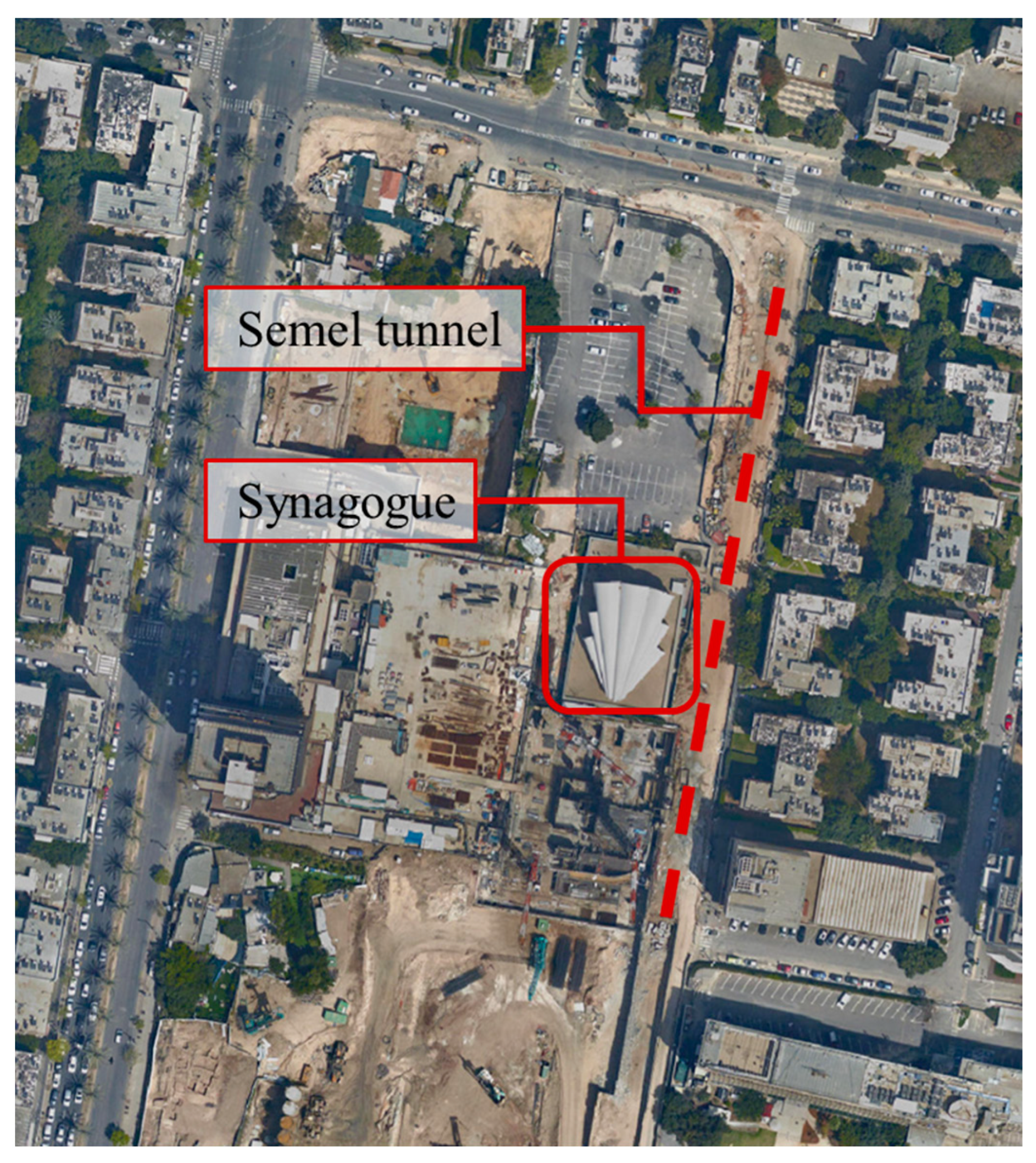
One of the main risks of deep excavations in a dense urban environment is that nearby structures can be negatively impacted by ground movements. Particularly, the Heychal Yehuda synagogue is highly sensitive to ground movements. The synagogue is situated approximately 3 m west of the Semel tunnel, and its basement floor lies on shallow foundations. Moreover, cracks have appeared in the synagogue walls even prior to the tunnel excavation works, most likely due to the excavations of high-rise buildings constructed on the southern and western boundaries of the synagogue. Figure 1 shows an aerial view of the Semel tunnel route and the adjacent synagogue structure.

The Semel tunnel project was not planned according to the observational method, and the traditional design–bid–build approach was implemented. However, due to the sensitivity of the synagogue structure, special considerations were made for this section. It was decided that in the vicinity of the synagogue, a top-down construction operation would be applied, consisting of two main stages: (1) minimal excavation to allow for the tunnel concrete slab to be constructed, and (2) excavation to the bottom of the tunnel, with the tunnel slab serving as lateral support. Figure 2 shows the formwork for the slab concrete during stage #1.

Based on SPT tests carried out on-site, input parameters were assumed, and geotechnical analysis was carried out. This analysis showed that the top-down method would induce small displacements, and it was, therefore, assumed that excavation would not risk the structural integrity of the synagogue. However, given the uncertainty of geotechnical works, an observational approach was adopted. A monitoring plan was devised, where tunnel wall displacements were measured, and vibrating wire crack meters were installed in the synagogue. Given a large displacement of the wall during the first stage and the appearance and/or elongation of cracks in the synagogue, a jet-grouting operation would be carried out to reinforce the soil beneath the synagogue basement. This operation would be used as a last resort, due to both the large cost of this operation and apparent risks due to possible improper application of the grouting. Ultimately, the top-down construction was recently completed without need of the grouting operation. It is noted that the first author was part of the project design team.

3. Methodology for Coupling FE and MLA Analysis

The idea of coupling numerical modeling with MLA has been discussed, tested, and implemented for different applications. The concept of surrogate models where MLAs are used to alleviate the burden of computationally expensive models has been developed [12]. Furtney et al. [13] discuss the use of surrogate models for rock and soil engineering applications and demonstrate three examples of predictive tasks: crushed zone size in rock blasting, the effective properties of a discrete fracture network (DFN), and the bearing capacity of a layered soil. Salazar and Hariri-Ardebili [14] used ML to construct a metamodel for assessing dam safety according to a statistical distribution of random variables. Tao et al. [15] used a particle swarm optimization algorithm to increase the accuracy of a tunnel deformation analysis. Mitelman and Urlainis [16] used numerical data to demonstrate that learning can be transferred from different but similar data sets.

For geotechnical operations, it is important to decide upon the suitable analysis methods. Whether using empirical, analytical, or numerical methods, it is common practice to compute results for a range of input parameters. For conventional projects, the engineers need to design according to a critical scenario and apply a suitable factor of safety to their design. In contrast, for projects where the observational approach is implemented, a range of possible outcomes are considered and prepared for.

Due to the inherent uncertainties associated with the selection of soil and rock input parameters, different probabilistic tools have been integrated within standard geotechnical analysis [17]. The probabilistic analysis is regularly used to compute the probability of failure [18].

Here, we propose automating the process of finite element (FE) modeling for ML analysis. The FE models must be staged according to the observational approach, where results from early stages of the project are used as a basis for assessing subsequent ground responses.

Prior to ML analysis, it is important to gain confidence that the FE models are acceptable. Hence, it is advised that a number of models be examined thoroughly to avoid the garbage in, garbage out phenomenon.

Once a series of FE models have been computed, three variables can be created:

• V1: initial deformation profile;
• V2: final deformation profile;
• V3: the input parameters (IPs) used for each model.

Table 1. Input and output variables for ML analysis.

Use	Input Data	Target Output
Feature importance	V3	V2
Deformation prediction	V1	V2

lists the two proposed ML analyses. By training variable V3 against V2, feature importance can be readily computed. Feature importance is the relative impact of each input parameter on the final outcome for that specific ML model and is often used for model interpretability. However, it can also be used to improve the performance of the ML model through feature selection, as well as to establish whether additional efforts should be invested in field investigations.

By training V1 against V2, final deformation predictions can be computed instantaneously based on deformations from previous stages. This obviates the time-consuming task of building, calibrating, and interpreting FE models manually. This is especially important for observational method projects, where decisions must be made promptly during the actual project construction.

Devising an effective monitoring plan is considered an essential part of applying the observational method. In addition to assisting the engineer during construction, the ML analysis for deformation prediction can provide valuable insights that can affect the monitoring plan. During this stage, different displacement results can be compared, and the deformations that serve as the best predictors of future failure should be selected for monitoring.

Both the quantity and quality of the data have a significant impact on the success of the subsequent stages of data analysis. With MLA, different sensitivity analyses can be carried out with the objective of investigating how many data points are optimal and how robust the model is in cases where noise is introduced to the data.

The flowchart in Figure 3 summarizes the proposed methodology.

Although numerous geotechnical modeling methods and techniques have been developed by many notable researchers, for many geotechnical engineering projects, it is difficult to accurately predict the physical outcomes (i.e., stresses, strains, and deformations) of construction. Due to epistemic knowledge gaps in the fields of soil and rock mechanics, this statement is true even for projects where rigorous field data are gathered prior to project execution [19]. The limitations of the proposed methodology will be discussed in Section 7.

4. Demonstration of Proposed Analysis

4.1. Data and Assumptions

In this section, we use the Semel case study as an example to demonstrate the use of the methodology proposed in the previous section. It is noted that the original data (i.e., geometry and strength parameters) have been changed, as the purpose of the current study is to demonstrate the use of ML for a practical application, and not to discuss the actual results in the Semel tunnel project. For the same reason, actual measured displacements are not presented in this paper.

The commercial code RS2 was used for the 2D FE analysis [18]. While tunnel analysis is essentially a 3D problem, a 2D plane-strain analysis is assumed to be sufficient for the current problem. An important advanced, built-in feature of the RS2 code is its ability to execute probabilistic analyses. Different statistical methods (e.g., point estimate, Monte Carlo, and Latin hypercube) and distributions (normal, uniform, etc.) can be used to automate the process of generating models with strength parameters that vary according to user preference.

Accordingly, one thousand FE models were automatically generated via the Monte Carlo method. The Monte Carlo method is an iterative process where random parameters are selected according to a statistical distribution defined by the user. It is emphasized that Monte Carlo analysis was used as a tool for generating the data set for the ML analysis. This is different from the traditional use of the Monte Carlo method as a probabilistic tool. For this reason, a uniform distribution was used for all parameters. While probabilistic analysis generally requires using normal distributions for geological materials, ML models perform better when trained on uniformly distributed data sets. The sixteen model input parameters are listed in

Table 2. Variables for data generation.

Entity	Property	Notation	Units	Minimum	Mean	Maximum
1. Fill	Young’s Modulus	E1	MPa	5	10	15
	Friction Angle (peak)	FA1	Degrees	25	30	35
	Cohesion	C1	MPa	NA	0	NA
2. Sand 1	Young’s Modulus	E2	MPa	30	40	50
	Friction Angle (peak)	FA2	Degrees	27.5	30	32.5
	Cohesion	C2	MPa	0	0.002	0.004
	Friction Angle (residual)	RFA2	Degrees	10	20	30
3. Sand 2	Young’s Modulus	E3	MPa	90	100	110
	Friction Angle (peak)	FA3	Degrees	30	35	40
	Cohesion (peak)	C3	MPa	0	0.02	0.04
	Friction Angle (residual)	RFA3	Degrees	10	22.5	35
	Cohesion (residual)	RC3	MPa	0	0.02	0.04
4. Joint	Normal Stiffness	JNS	MPa	20	40	60
	Shear Stiffness	JSS	MPa	2	4	6
	Friction Angle	JFA	Degrees	15	20	25
5. Earth Pressure	K Ratio	K	-	0.4	0.5	0.6

. A Mohr–Coulomb plastic failure criterion was assigned to the soil materials in the model. The fill layer was cohesionless. The mean relative minimum and relative maximum values are given in the table as well. For the structural elements, the input parameters of the concrete material were constant for all models. The concrete Young’s modulus and Poisson ratio were assigned values of 30 GPa and 0.25, respectively. The thickness of the tunnel walls and ceiling were 0.6 and 0.45 m, respectively.

In regular practice, it is generally instructed to assume a normal distribution for soil strength parameters [17]. However, the objective of the current automated modeling process was to generate data for MLAs to train and test on. Training the data on normally distributed data would favor prediction of data close to the mean, at the expense of the accuracy of the data farther away from the mean. However, the primary concern during construction is to capture the extremes (i.e., high redundancy vs. unacceptable risk). A uniform distribution ensured a balanced data set for the ML analysis.

The parameters of each of the three soil layers were varied for the model analysis. For all soil materials, the Mohr–Coulomb elastoplastic model was used. More advanced constitutive models for soils, such as the Hardening Soil model, have been found to be more accurate in terms of displacement prediction. However, the traditional Mohr–Coulomb failure criterion has been found to yield acceptable results for tunneling problems [20]. Switching to a more advanced material would require re-evaluating MLA performance. Complex failure models require a greater number of inputs with nonlinear relationships, which may necessitate using more sophisticated MLAs, as well as generating more data.

In order to model the interface between the wall and the soil, a joint boundary was defined in the model. The joint boundary stiffness is a numerical construct intended to simulate the relative slip within a FE mesh. The friction angle at the wall interface can be estimated using empirical guidelines (e.g., see [21]).

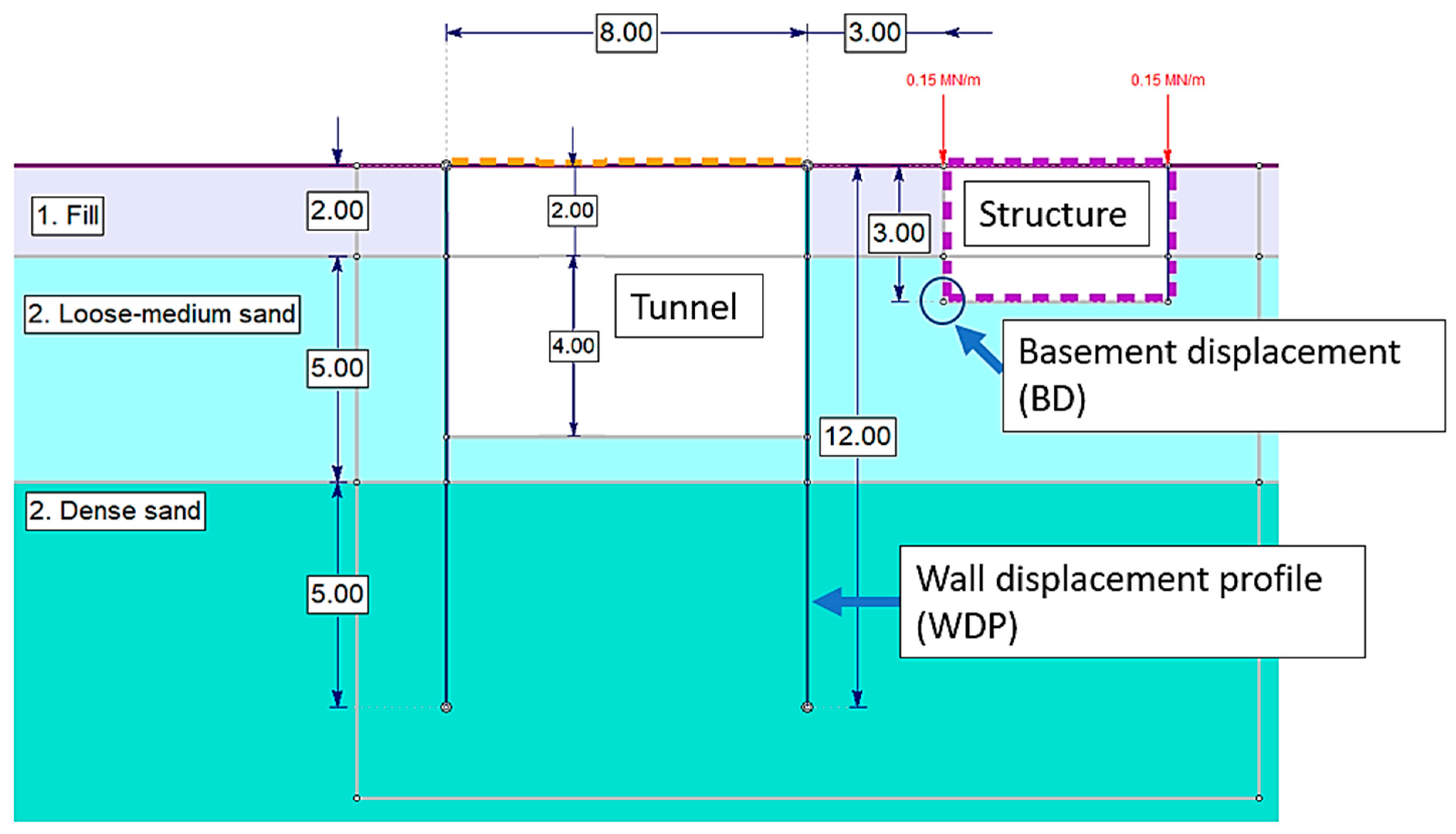
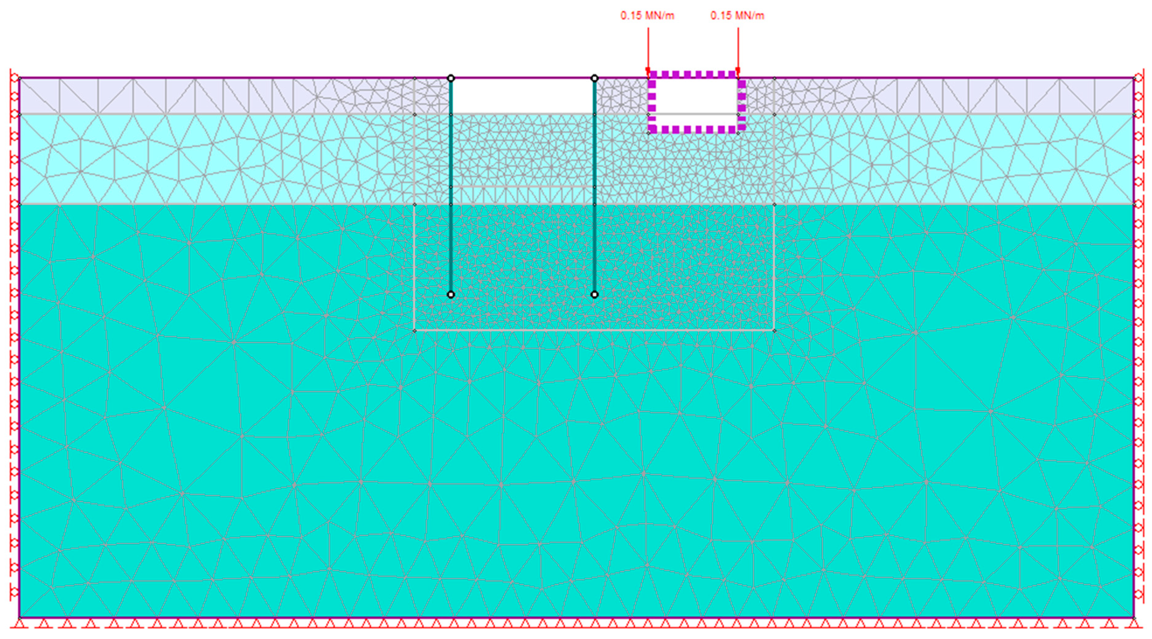
Figure 4 shows the problem geometry, and Figure 5 shows the FE model and mesh. The models consisted of 3169 elements and 12,748 degrees of freedom. The model was divided into four modeling stages:

• Stage #1: preliminary geostatic stage;
• Stage #2: installation of tunnel walls and loading of the adjacent structure;
• Stage #3: initial excavation stage to a depth of 2 m from surface level;
• Stage #4: construction of the upper tunnel slab and final excavation to the bottom level of the tunnel.

During the solving process, result files with stresses, strains, and displacements for each node were generated and stored as text files. A Python script was created to collect the relevant results and organize the data in the proper form for ML analysis. In order to avoid collecting meaningless results, non-converging models were checked for. For the current work, all models converged. Three main variables were generated through this process: (1) the wall displacement profile (WDP) recorded in Stage #3, (2) the basement displacement (BD) recorded in Stage #4, and (3) the input parameters (IPs) used for each model.

The WDP and BD are shown in Figure 4. The BD represents the resultant horizontal displacement of the structure adjacent to the tunnel and the WDP is the full horizontal displacement profile measured at 25 points along the wall. The objective of the ML model was to predict the BD on the basis of the measured WDP. Succeeding in this task would, therefore, imply that an engineer could accurately predict the final displacement of the adjacent structure. Subsequently, the engineer should compare the predicted deformation to the predetermined critical deformation. In the current example, if the BD was predicted to be greater than the acceptable deformation, a grouting operation was set forth.

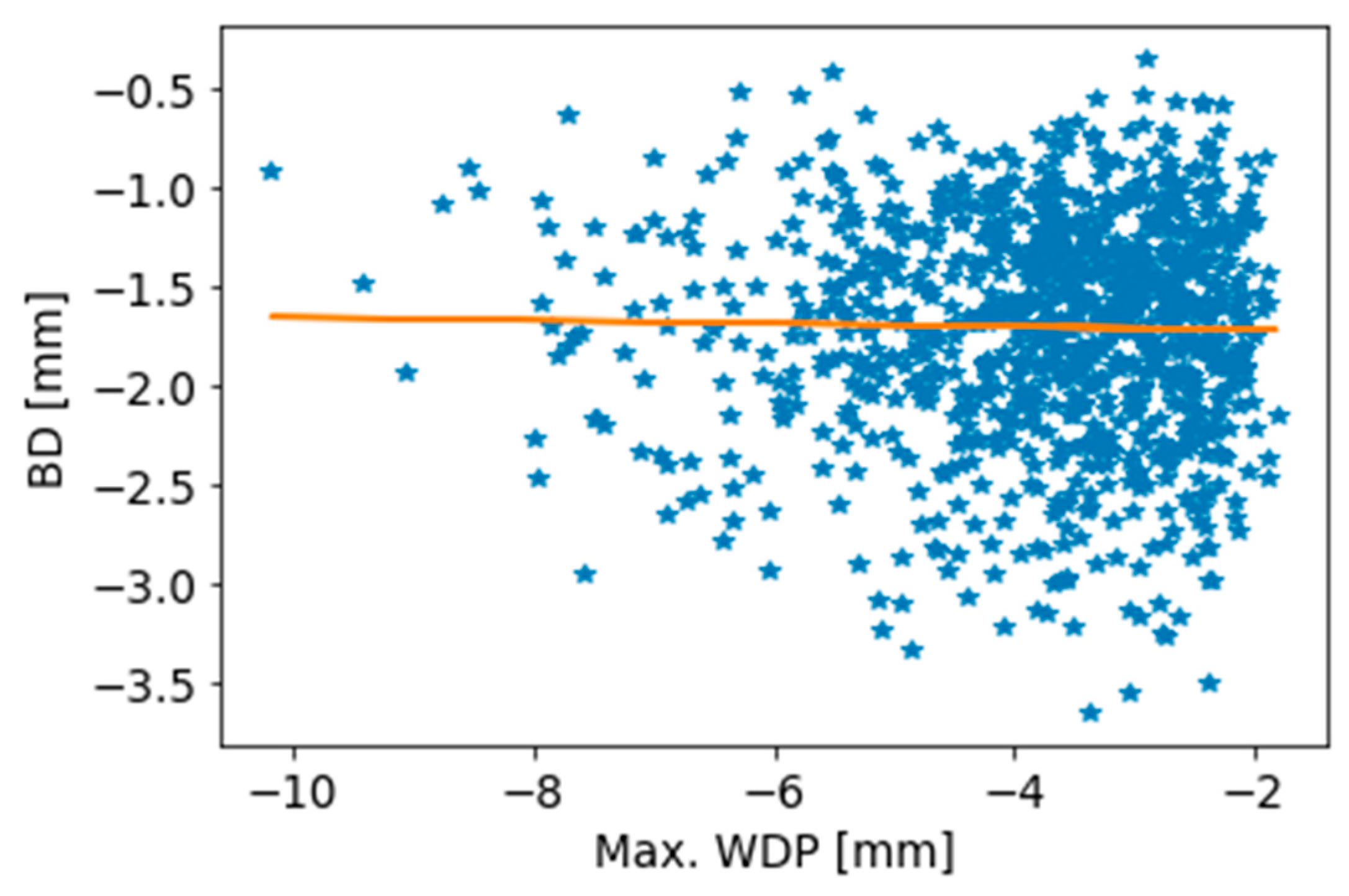
Figure 6 shows a plot of the BD with respect to the maximum value from the WDPs. This plot is useful, as it visualizes the anticipated ranges of displacements. The linear fit shown in Figure 6 shows that no simple linear correlation can be applied between the two deformations. A near-zero coefficient of determination (R²) of 0.002 was computed for these data, suggesting that a more advanced ML scheme was needed.

The results shown in Figure 6 demonstrate how the proposed methodology may provide nontrivial insights for the development of a monitoring plan. Empirical investigations conducted by others have shown that for the problem described here (a flexible cantilever wall), the maximum value of the WDP occurs at the point of the top of the wall [21]. In situ data collection requires devising a firm understanding of the available monitoring methods and their accuracy and limitations [22]. The maximum WDP could be obtained manually, by measuring the deformation at the top of the wall. Measuring the full WDP requires the installation of suitable monitoring devices, such as inclinometers. Another important capability of inclinometers with respect to ML analysis is that the recorded data can be transmitted in digital form, allowing for further computer processing. Obviously, additional monitoring has budgetary consequences and is justified only if it aids the engineer in the decision-making process. Figure 6 illustrates that the full maximum displacement serves as a poor predictor, indicating that a more rigorous monitoring plan must be employed.

We, therefore, define the data set according to the full WDP. The size of the data set in this example depended on the matrices of the WDP and BD. The number of columns in the WDP represented the number of data points along the tunnel wall profile (equal to the number of nodes in the FE model, as shown in Figure 4). The BD was a single-column vector. The number of rows in the WDP and BD were equal to number of FE models.

For ML analysis, the random forest (RF) regression type model was used. The decision tress were ML models used for both classification and regression. Decision trees predict the value of a target variable by learning simple decision rules inferred from data features. The tree is built by splitting the data, constituting the root node of the tree, into subsets. This process is repeated in a recursive manner. The number of splits in a decision tree are referred to as the tree depth. Random forest (RF) models consist of multiple decision trees. For regression tasks, the average prediction of individual trees is calculated. An individual decision tree is prone to overfitting, and, therefore, using a group of trees reduces the overfitting overall because the algorithm averages the results of each tree in the RF. RFs generally outperform decision trees and are considered more robust models. For engineering applications, RFs have been found to outperform other MLAs, such as support vector machines and extreme gradient boosting [23]. For the purpose of this paper, RFs were chosen because of their robust and interpretable nature, as well as their ability to perform well with minimal hyperparameter tuning. A maximum tree depth of 60 was chosen for the RF model, and no hyperparameter tuning was carried out. Hyperparameters are parameters that control the learning process of the MLA and are not part of the problem.

The open-source Python programming language was used for data preprocessing and MLA application. The Scikit-learn library was used to import the functions for the execution of the RF model.

It is the authors’ opinion that a culture of data sharing should be encouraged in order for the benefits of ML to be utilized for the progress of geotechnical engineering [24]. In accordance with this view, we intend to provide our basic script upon request to the corresponding author to allow for other researchers and practitioners to further build upon our work.

4.2. Results

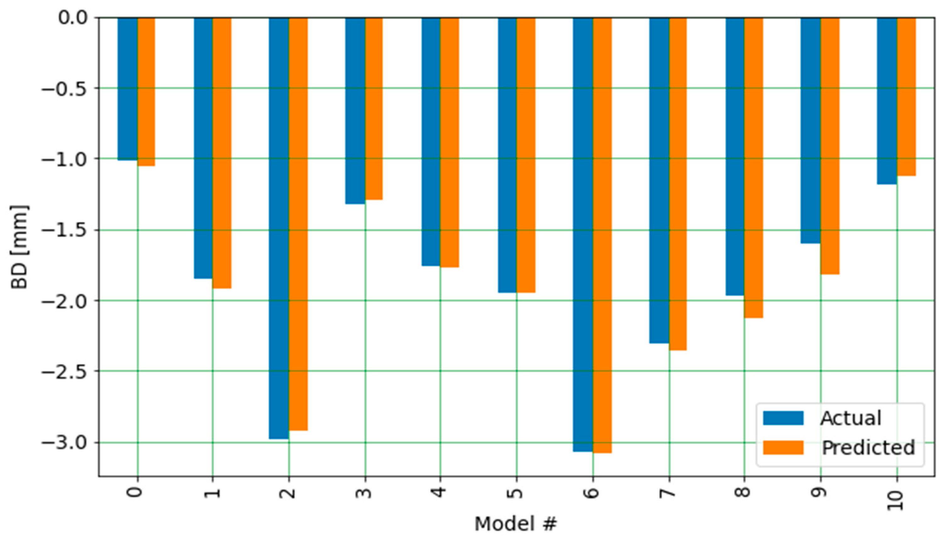
The RF model was trained on 800 FE models and tested on 200 to predict the final deformation (BD) from the initial deformation (WDP). For the purpose of keeping the model simple, no cross-validation, hyperparameter tuning, or feature selection were performed. Figure 7 shows a comparison of the actual results of the BD vs. the corresponding results predicted by the ML model for 10 FE models that were randomly selected from the test set.

In general, the predicted BD values closely matched the actual values. However, checking for all predicted values shows that the trained RF model fell short when predicting the most extreme values. The predicted and actual values had the closest match at final deformation values ranging from approximately 1 to 3 mm. This is consistent with the distribution of the final deformation values used in this exercise, where around 90% of the values fell in this range, as shown in Figure 8.

The mismatches between the predicted and actual values shown in Figure 7 tended to result from the model overpredicting the final deformation. In the context of this problem, an overprediction is considered acceptable because it lends to a more conservative design.

A number of metrics are available for evaluating model performance, including mean square error, root-mean-square error (RMSE), and more. Here, we used the coefficient of determination R² as well as the RMSE. The R² coefficient is calculated as:

$${\mathrm{R}}^2=1-\frac{{SS}_{res}}{{SS}_{tot}}$$

where ${SS}_{res}$ is the sum of squares of the residuals, i.e., the difference between the actual and predicted values, and ${SS}_{tot}$ is the total sum of squared differences. R² provides a straightforward assessment of the ML model performance; a result of one indicates perfect accuracy, and a result of zero indicates no correlation whatsoever. Note that negative values of R² are possible, inferring a model that has worse predictions than the baseline zero. RMSE is calculated as:

$$\mathrm{R}\mathrm{M}\mathrm{S}\mathrm{E}=\sqrt{\frac{\sum (y_i-{\widehat{y}}_i)}{n}}$$

where n is the number of data points, $y_i$ is the actual value, and ${\widehat{y}}_i$ is the predicted value. Compared to R², RMSE has the advantage of being in the same units as the predicted variable, rendering it more interpretable.

The R²s for the training and testing data sets were 0.97 and 0.76, respectively, while the RMSE for the training and testing data sets were 0.0000974 and 0.000266, respectively.

These results indicate some minor overfitting. The test data results are considered acceptable for the problem at hand. Possibly, higher accuracy could be obtained through methods such as hyperparameter tuning and feature selection [25].

The amount of data to be collected is a fundamental question that lies in the basis of any data-scientific research project. Pre hoc sample size determination is generally regarded as an unsolved challenge in the field of data science [26]. Therefore, each problem requires determination of the sample size via post hoc testing. In order to investigate the effect of the number of samples (i.e., FE models) on the model performance (R² and RMSE), an iteration where a subset of the total number of FE models for training and testing was increased from 50 to 1000 in increments of 10 was created. For each iteration, the data were split into 80% for training and 20% for testing. The results of this analysis are shown in Figure 9.

As can be seen from Figure 9, there was significant variation in the R² and RMSE values for data sets with up to 200 samples. After 600 samples, the R² and RMSE values generally converged to greater values of around 0.8 and 0.00025, respectively. These results demonstrate that MLAs are capable of accurately predicting the BD from the WDP. Comparing these results with those shown in Figure 6 shows that when monitoring the full WDP, in contrast to measuring only the maximum wall displacement, deformation predictions can be accurately made with fewer than 1000 FE models. Note that the results are not smooth, as MLAs use iterative and randomized methods for data fitting.

Numerical simulations are inherently noisy, due to various effects (e.g., mesh dependence, boundary effects, etc.). However, real-world settings are regularly found to be considerably noisier. Sources of real-world noise may include the inherent heterogeneity of geological materials, complex time-dependent behavior, the impact of construction vibrations on the monitor device output, readings from uncalibrated monitoring devices, etc. It is, therefore, emphasized that ML analysis can help set a lower bound for an on-site monitoring plan, and depending on the degree of noise, it is possible that a considerably greater amount of data would need to be collected for ML analysis. The proposed methodology limitations are further discussed in Section 7.

5. Feature Importance Analysis

Feature importance in an ML model allow us to better interpret the model and determine which features have a bigger impact on the model’s predictions. This can aid engineers in improving the performance of both the FE and the ML modeling by focusing efforts on obtaining better-quality data for the features that are important. The computational technique for feature importance was first published by [27].

The input parameters for the feature importance analysis were those listed in Table 2. An additional RF model was generated, where the input parameters were used as the input to predict the final deformation (BD). Similar to the RF model in the previous section, the data set was divided into 80% for training (800 samples) and 20% for testing (200 samples), and no hyperparameter tuning, cross-validation, or feature selection were performed for the sake of simplicity. Similar to the RF model in the previous section, there was a generally close match between the predicted and actual BD values, but the model was unable to capture the extreme values.

The Scikit-learn feature importance function was used for the feature analysis. The results of the feature analysis are shown in Figure 10. The results show that the most important feature for the model prediction was the joints’ normal stiffness. This variable is a fictitious numerical entity intended for simulating relative slipping between the tunnel wall and soil. Reliable estimation of this parameter is difficult, and there are only general recommendations for estimating joints’ boundary stiffness [18]. If real-world deformation data are collected from a similar geological formation, it would be advisable to compare model results and consider rerunning models with a different range of normal stiffness of joints to see if this improves the model’s accuracy.

The second significant variable was the lateral earth pressure coefficient Ko. This variable manifests a material property that could be measured in situ or assessed according to different empirical formulae. Hence, depending on the project characteristics and constraints, consideration should be given to whether it would be effective to carry out in situ testing to reduce the uncertainty of Ko.

The other parameters were found to be considerably less significant. This suggests that the material properties (e.g., Young’s modulus, friction angle, cohesion, etc.) of the soil layers have a slight impact on deformation results, and that reducing their uncertainty in this case would be ineffective.

It is important to bear in mind that feature importance results are highly dependent on the model and specific data set. Feature importance does not provide a mechanistic understanding of the problem; rather, it is mainly used for better understanding how the model made predictions. Even small changes in the range of input parameters can highly alter feature importance. Hence, broad conclusions from feature importance must be avoided.

6. Summary and Conclusions

The observational method is an approach developed to allow geotechnical engineers to modify a design during project construction according to monitored data. Although it has economic appeal, this approach is not widely applied in practice. In this study, MLAs were coupled with FE modeling in order to enhance the modeling process and to aid the engineer in the decision-making process during the application of the observational method. Specifically, two important tasks were automated: determining model’s feature importance and predicting final deformations from preliminary deformations.

Feature importance can readily be calculated using RF models. The results of feature importance could be used to determine whether additional field data collection and/or modeling would be effective for reducing the uncertainty of impactful input parameters.

Implementation of the observational method requires that decisions for later stages of the project be made based on observations of the ground response during earlier stages of construction. Accordingly, the engineer must determine whether ground conditions are within the acceptable range or require the application of predetermined contingency actions. Increasing the ability to predict final deformations from these observations can greatly assist the engineer in the decision-making process. For this purpose, MLAs can be trained and tested on FE models to establish a mathematical relationship between deformations in the preliminary and final stages.

The case study of the Semel cut-and-cover tunnel was used as an example for the demonstration of the proposed analyses. For this example, ML analysis showed that the maximum tunnel wall displacement alone was not sufficient for establishing a correlation with the final displacement of the structure adjacent to the tunnel, and the full tunnel wall displacement profile was necessary. This demonstrates how ML analysis can assist in developing a monitoring plan that collects the essential data for optimal decision making.

When considering the full wall displacement profile, it was found that accurate and non-trivial deformation predictions could be obtained with the RF MLA. A database of 1000 FE models was generated, and it was found that fewer models are sufficient for successful MLA performance. The RF models did not perform well with the extreme values, indicating that it would be good practice to extend the range of the estimated input parameters for better ML performance.

7. Limitations

The past decades have witnessed the increased digitization and digitalization of geological engineering processes [19]. Kant and Kerr [28] discussed the epistemic problem of perceptual tasks performed by different software and concluded that automated data interpretation processes should not replace human engineering judgment. For the field of geotechnical engineering, acknowledging limitations and applying critical thinking and expert judgment is particularly important, as the consequences of an engineering failure can be catastrophic. Actual decision making based on monitoring data and numerical modeling requires a clear understanding of knowledge gaps and limitations.

The methodology of ML integration proposed in the current paper is intended solely for the objective of accelerating engineering modeling tasks for geotechnical projects.

The proposed methodology helps to increase predictive power only if the models themselves are acceptably accurate. Ultimately, any limitation that applies to geotechnical analysis via FE modeling cannot be eliminated by MLAs.

Another important limitation is related to the technical process of generating numerical data. At the current state of practice, numerical packages can be categorized into three classes:

• Codes that have application programming interfaces (APIs) for external programming;
• Codes that do not have an API but generate text files that can be subject to external coding;
• Closed codes that are not open to any type of interfacing.

With regard to the coupling of ML with numerical modeling, it is generally required that the code belong to classes 1 or 2; otherwise the user would not be able to generate and prepare data for ML applications. The RS2 code used for the current study belongs to the second class; hence, the modeling automation and manipulation were limited to the available features of the program. The authors, therefore, encourage research and commercial developers to make their codes open for API interface, which enables manipulation and analysis, and develop built-in ML features to assist users that wish to do so.