

Cyclic Steps Created by Flowing Water on Ice Surface


1
Graduate School of Engineering, Hokkaido University, Sapporo 060-0813, Japan
2
Faculty of Engineering, Hokkaido University, Sapporo 060-0813, Japan
*
Author to whom correspondence should be addressed.
†
These authors contributed equally to this work.
Geosciences 2023, 13(5), 128; https://doi.org/10.3390/geosciences13050128
Submission received: 15 March 2023
/
Revised: 11 April 2023
/
Accepted: 24 April 2023
/
Published: 28 April 2023
Abstract
:The interface between ice and fluid can become unstable and devolve into cyclic steps bounded by hydraulic jumps. These steps are created by flowing water or wind over the ice surface. This study presents an analytical model to reproduce cyclic steps created by water over the ice surface. We apply four governing equations: the momentum equation, the continuity equation, the heat transfer equation in water, and the energy balance equation (the Stefan equation). After calculation, we can generate the variations in the depth-averaged water temperature, the depth-averaged velocity, and the ice elevation over one step wavelength. We can also understand the cyclic step formation process and how the heat transfer capacity of air and water, and the Froude number in the normal flow condition influence the wavelength. The results of the obtained steps in the analysis are compared with experimental observations to validate our model.
1. Introduction
Boundary waves forming on the ice are often observed. Carey et al. [1] found ripples and dunes on the underside of the river ice cover in the St. Croix River. Gilpin et al. [2] conducted experiments and linear stability analysis on the formation of waves at an ice–water interface. The interaction between the ice surface and flow causes heat transfer variations, leading to the formation of waves. Comporeale et al. [3] performed a linear stability analysis of ice ripples formed by water. They pointed out that the ice–water interface can be unstable in the case of laminar flow at large Reynolds numbers ().
Cyclic steps are also a type of boundary wave that can be observed on ice. They are a train of self-generated rhythmic bedforms bounded by hydraulic jumps. These steps have been reported on erodible beds in channels [4], on the subaqueous ice-contact fan [5], on the seafloor in response to turbidity currents [6,7,8], at deltas [9,10], on volcano flanks [11], and in the depositional record of fluvial environments [12,13]. Our study focuses on cyclic steps on the ice. The steps due to a superglacial meltwater stream are found by Kalstrom et al. [14]. The flat ice surface becomes unstable after the water flows through, forming a series of steps on the ice–water interface. Spiral troughs created by the katabatic wind on Mars’s north polar ice cap surface are interpreted to be cyclic steps (Figure 1a) [15,16]. The solidification and sublimation of water vapor contained in the katabatic wind cause the formation of these steps. In addition, the Coriolis force is the primary influence on direction, allowing the flow to take a spiral path. On the Antarctic ice sheet, similar bedforms formed by the katabatic wind are discovered [17,18].
The understanding of cyclic steps has significantly benefited from laboratory experiments and models. Taki and Paker [19] conducted experiments to reproduce transportational cyclic steps associated with the suspension and deposition of sediment. They presented that cyclic steps are considered permanent, long-wave features and migrate upstream without changing form. Parker and Izumi [4] introduced a model to analyze cyclic steps formed purely by erosion on cohesive soil in open channel flow and proposed to use threshold velocity to determine the wavelength of one step. This threshold velocity corresponds to the longest wavelength in the calculation. Sun et al. [20] developed a general theory to explain the formation regime and most features of transportational cyclic steps related to suspended sediment. On the upstream side, slow flow causes deposition, while erosion caused by swift flow occurs on the downstream side. Wu and Izumi [21] proposed an analytical model to reproduce cyclic steps formed by long-runout turbidity currents. They presented that steeper bed slopes facilitate the formation of shorter wavelengths, and this has been validated in comparison with the natural field.
Figure 1.
Cyclic steps in natural fields and experiments. (a) Spiral troughs on the north polar ice cap of Mars. By NASA/JPL-Caltech/MSSS. https://www.nasa.gov/mission$_$pages/MRO/multimedia/pia13163.html, accessed on 7 March 2023 (b) The experiment of cyclic steps on ice [22]. 240 min subsequent to run initiation (run number CSIM120908A). Flow is left to right.

The formation process of cyclic steps on ice is similar to that of transportational cyclic steps formed by sediment transport (e.g., [20,21]). The erosion and deposition of sediment result in the formation of cyclic steps, and the conservation of bed sediment is described by the Exner equation. The formation of cyclic steps on ice is not only a mechanical but also a thermodynamic process. Heat transfer causes melting and freezing to form cyclic steps, and the energy balance can be governed by the Stefan equation [22]. Based on our understanding, few studies about cyclic steps on ice exist. Cyclic steps usually migrate upstream without changing form, while Naito et al. [23] conducted experiments and proposed a model to research downstream-migrating steps on ice. Yokokawa et al. [22] produced steps on icy substrates in the laboratory (Figure 1b) and presented a linear stability analysis to explain the precursors of cyclic steps, upstream-migrating antidunes. They elucidated that the boundary between ice and water is unstable to perturbations under Froude-supercritical flow and investigated the instability of the interface between ice and water. However, cyclic steps themselves cannot be described in terms of linear stabilities since they are a fundamentally nonlinear phenomenon, and the discontinuity at each hydraulic jump prevents the Taylor expansion on the base state. Experiments related to the cyclic steps formed by wind are conducted by Sumida et al. [24]. They simulated wind on ice in experiments and found that longer wavelengths appear on steeper slopes.
Boundary waves created on ice by water or wind are both associated with heat transfer. However, it is difficult to know the variables in the normal flow condition for the cyclic steps formed by the wind. To study the basic knowledge about geological features caused by heat transfer, we propose an analytical model to reproduce the formation of cyclic steps by water over an ice surface. The linear stability analysis presented by Yokokawa et al. [22] cannot be regarded as a direct study of cyclic steps themselves. Hence, we refer to the model of Naito et al. [23] to apply the depth-integrated flow equations, the depth-integrated heat transfer equation, and the Stephen equation. The empirical formulas are used to describe the heat flux in water, ice, and ambient air.
The theory of Naito et al. [23] states that step wavelengths depend on the water velocity before hydraulic jumps, but they did not present a method to determine wavelengths. Therefore, we aim to overcome this problem in this study. In the analysis, the wavelength could reach a maximum value along with the variation of the temperature downstream of the hydraulic jump. We use this longest wavelength for analysis. The data from Yokokawa et al.’s experiments [22] are used to validate our model.
2. Methods
2.1. Formulation
2.1.1. Governing Equations
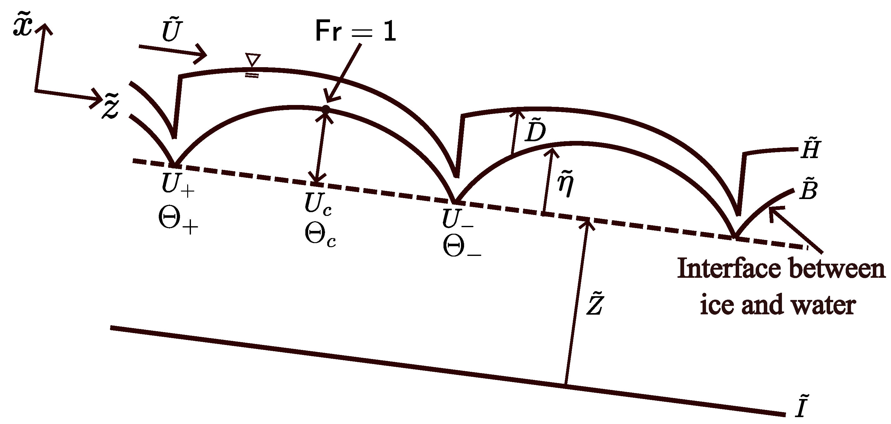
Suppose that a steady, uniform Froude-supercritical flow runs over a flat ice surface, as shown in Figure 2. The surface becomes unstable to give rise to a spontaneous formation of a series of steps, and the permanent presence of hydraulic jumps stabilizes the steps. At the interface between water and ice, solidification and melting are taking place at the same time. In our assumption, the fluid temperature is lower than the surrounding air and higher than the ice temperature. Similar temperature distributions can be observed on the spiral troughs of Mars [16].
The linear stability analysis presented by Yokokawa et al. [22] cannot describe cyclic steps themselves. Hence, to directly analyze cyclic steps on the ice, we refer to the approach of Naito et al. [23]. The scale of the streamwise direction is much larger than the scale in the upward direction, and we thus integrate the Navier–Stokes equations and the heat equation of flowing water from the ice surface to the water surface. The focus is on the variation in the streamwise direction, such as velocity, water temperature, ice elevation, and water depth.
The flow configuration is described by the shallow water equations as shown here:
where is the time, is the coordinate in the streamwise, is the depth-averaged velocity component in the coordinate, is the flow depth, is the density of water (=1000 kg/m3), g is the gravity acceleration (=9.8 m/s2), is the ice elevation, s is the slope of the channel, is the bed shear stress, and means dimensional variables and is later removed to denote dimensionless variables. Since the scale in the streamwise direction is much larger than that in the depth direction in the shallow water approximation, the boundary layer of the flow quickly develops in the streamwise direction. Therefore, because the boundary layer can be assumed to be already in equilibrium, it is possible to ignore the effect of boundary layer development in the shallow water approximation.
The heat flux variation in the vertical direction is much faster than that in the streamwise direction. Therefore, the integration approach, as in the shallow water equation, is applied to the heat transfer equation in the flowing water. The derivation is in Appendix A. The heat equation in water is
where is the depth-averaged water temperature, is the heat flux in flowing water in the depth direction .
The heat flux difference is the key to forming cyclic steps. The difference between the heat flux coming from the ice below to the water–ice interface and that going out from the interface to the water above causes the phase change of water, melting, and solidification. The time evolution of the water–ice interface due to the phase change is described by the Stefan condition of Equation (4).
where is the latent heat of melting, is the density of ice, is the heat flux within the ice in the direction.
There are three unknown terms related to heat flux , , in Equations (3) and (4). We define them by empirical formulas. A boundary layer above the water surface produces a significant difference between the air and water surface temperatures. It is known that the heat flux from the ambient air to the water depends on air velocity and air temperature distributions. However, obtaining this information is difficult, so we employ a simplification discussed below, as Yokokawa et al. [22] performed. The heat flux from the surrounding air to the water surface is assumed to match that from the water surface to the flowing water. Since most studies focus on heat transfer from a solid surface to a fluid rather than between air and water, we use a formula in oceanography or geophysics here:
where is the air temperature, is a bulk heat transfer coefficient of air (=), is the air density (=1.29 kg/m3), is the specific heat of air (=1005 J/kgK), is a normalized heat transfer coefficient which is influenced by the wind speed. Assuming the wind speed is from 1 to 10 m/s, we find takes a range from to [25]. It follows that the value of is from 1.94 to 18.15.
A formula estimates the heat exchange flux between ice and water in the following forms:
where is the temperature at the ice–water interface and kept to the melting point, is a bulk heat transfer coefficient of water above the ice surface (), is the specific heat capacity of water (=4184 J/kgK), is a dimensionless ice–water transfer coefficient. Shirasawa et al. [26] presented that used in Resolute Passage, Northwest Territories, Canada was . Hamblin el al. [27] found that between a lake and an ice sheet was . Li et al. [28] proposed that at the ice–water interface at low-flow velocities (0.024 m/s–0.110 m/s) is .
Heat conduction is a significant means of heat transfer within a solid object, and Fourier’s Law is commonly used to describe heat conduction. Therefore, we apply Fourier’s Law here to describe the heat transfer within the ice, as shown below.
where is the temperature at the ice bottom, is the thermal conductivity of ice (=2.22 W/(mK)), and is the ice thickness.
2.1.2. Normalization
The following normalizations are introduced:
where the subscript 0 denotes variables in the normal flow condition (steady, uniform) before the development of steps, and is the drag coefficient. The shallow water approximation allows the above relationship between the bed shear stress and the flow velocity. The bed shear stress is related to the drag coefficient, which is generally a weak function of the flow depth relative to the roughness height. However, in this study, we assume the drag coefficient is a constant for simplicity.
We apply the quasi-steady approximation in governing equations. The water discharge is assumed to be constant, and the evolution of the ice surface is much slower than the flow change. Thereby, the flow is assumed to be steady, and we can drop the temporal terms in governing equations except in the Stefan equation. With the aid of Equations (8)–(13), Equations (1)–(4) can be rewritten to
where is the Froude number associated with the normal flow before the development of steps, is the normalized ice–water heat transfer coefficient, is a non-dimensional parameter representing the ratio of the air–water heat transfer coefficient to the water–ice heat transfer coefficient, is a non-dimensional parameter defined as the ratio of the thermal conductivity coefficient to the heat transfer coefficient in the water, which read, respectively,
Yokokawa et al. [22] observed cyclic steps on the ice migrating in the upstream direction without changing form. This is mainly because the water temperature is higher than the ice but lower than the air. The ice bed in the shallower supercritical flow is more affected by high atmospheric temperature than in the deeper regime. In contrast, Naito et al. [23] observed cyclic steps migrating downstream because the air temperature is lower than the melting point. In the experiments of Yakokawa et al. [22], the entire ice surface moves downward, since the heat flux from water is not necessarily balanced with that of ice. More specifically, vertical degradation is more active than upslope progradation. To describe these features of upstream-migrating cyclic steps, we refer to the study of transportational cyclic steps over an erodible bed [Sun and Parker, 2005] [20] and introduce a moving coordinate system, as shown here:
where f is the normalized migration speed in the streamwise direction, and is the normalized degradation speed of the ice surface in the depth direction. This transformation is applied to the governing equations, dropping the hat for simplicity. The governing equations (Equations (14)–(16)) keep the same form, but the Stefan equation (Equation (17)) is rewritten into
where is used to present the sum of the heat flux from the ice surface to the ice bottom and the migration speed of the ice surface in the depth direction for simplicity (). In the normal flow condition, the gravity force is in balance with the shear stress (. Hence, with the aid of Equation (13), we find
The heat transfer equation in water takes the form
2.1.3. Boundary Conditions
The subcritical flow continues to accelerate to become supercritical. The flow transits through a hydraulic jump from the supercritical to the subcritical regime, as shown in Figure 2. The momentum conservation between the upstream and the downstream of the hydraulic jump is
where subscripts − and + denote the upstream and downstream sides of the hydraulic jump, respectively. The normalized boundary condition is written to
As shown in Figure 2, the coordinate system’s origin is the downstream side of the hydraulic jump, and the ice elevation is taken to be zero before and after the hydraulic jump. The boundary condition of the ice elevation is
We assume the water temperature is continuous before and after the hydraulic jump, as shown below
2.2. Solution Method
The Froude number is vital in forming cyclic steps, since the critical Froude number is the key to discriminating the supercritical and subcritical flow. The method to solve this problem is based on the approach of Sun and Parker [20] to some extent. At the Froude critical point (i.e., ), the denominator of Equation (25) vanishes. In order to avoid this singularity, the numerator has to vanish at once. Thereby, we can calculate the velocity at the Froude critical point and the migration speed f, as shown bellow.
Here the subscript c denotes variables at the Froude critical point.
The governing Equations (23), (25) and (26) with the boundary conditions (28)–(30) form a two-point boundary value problem. The three boundary conditions are all the relationships between the variables before and after hydraulic jumps, rather than specific values of variables. Therefore, the wavelength of one step cannot be determined by these weak boundary conditions. The wavelength of one step is defined as the distance between two adjacent hydraulic jumps. One more boundary condition is necessary to close the problem.
In the study of cyclic steps created by flow over a cohesive bed [4], the threshold velocity, which denotes the onset of bed erosion, identifies the wavelength. However, there is no threshold velocity associated with the formation of cyclic steps on the ice. To overcome this deficiency, we assume the value of as one more boundary condition.
We solve this problem by the shooting method with the Newton–Raphson scheme. The flow in the normal flow condition is in the supercritical regime, so should be larger than unity. The calculation starts from the vicinity of the Froude critical point to avoid singularity. The temperature gradient and the ice elevation gradient at the Froude critical point are expressed in the following forms with the aid of Equation (26) and Equation (23), respectively:
The velocity gradient cannot be calculated at the Froude critical point by taking the limit . To allow a smooth transition across the Froude critical point, we apply L’Hopital’s rule to Equation (25). The gradient evaluated at the Froude critical point must satisfy the relation
where denotes at the Froude critical point. Since the flow transits from a subcritical to supercritical regime at the Froude critical point, the solution for at the Froude critical point should be real and positive.
Governing equations are integrated toward downstream and upstream directions until specified boundary conditions are met. We simultaneously adjust the guessed values of and to obtain the correct values. After the calculation, the variation of the water velocity, the water temperature, and the ice elevation can be obtained.
3. Results
3.1. Calculation for Wavelength
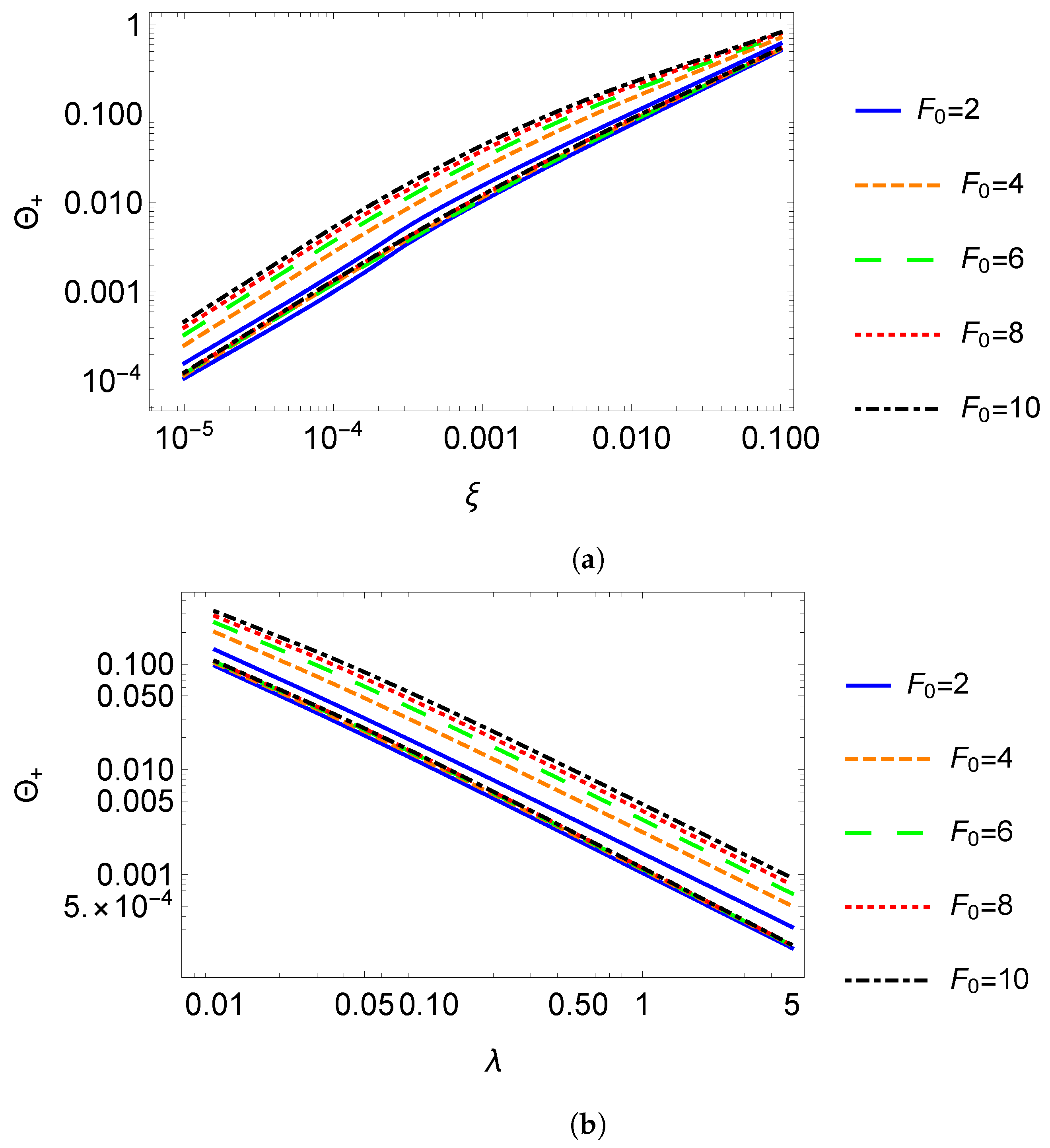
During the analysis, the temperature downstream of the hydraulic jump cannot be arbitrarily selected. We identify specific ranges for , as shown in Figure 3, which must be met for a solution to exist.
There is an explanation for the upper limit of . In the calculation, we find that a negative value for migration speed f leads to no solution. In addition, solutions reveal that the temperature variation over one step always exhibits a distinct feature, where is higher than , and the lowest water temperature is at the point . By using Equation (32) and establishing the relationships between and , we obtain . Therefore, exceeding the upper limit for results in a negative f value and no solution for the analytical model.
Moreover, there is a lower limit for . The average water velocity continues to increase until it is upstream of the hydraulic jump. Therefore, the numerator of Equation (25) should not be zero except at the Froude critical point. However, if is less than its lower limit, the numerator of Equation (25) is zero at a point other than the Froude critical point.
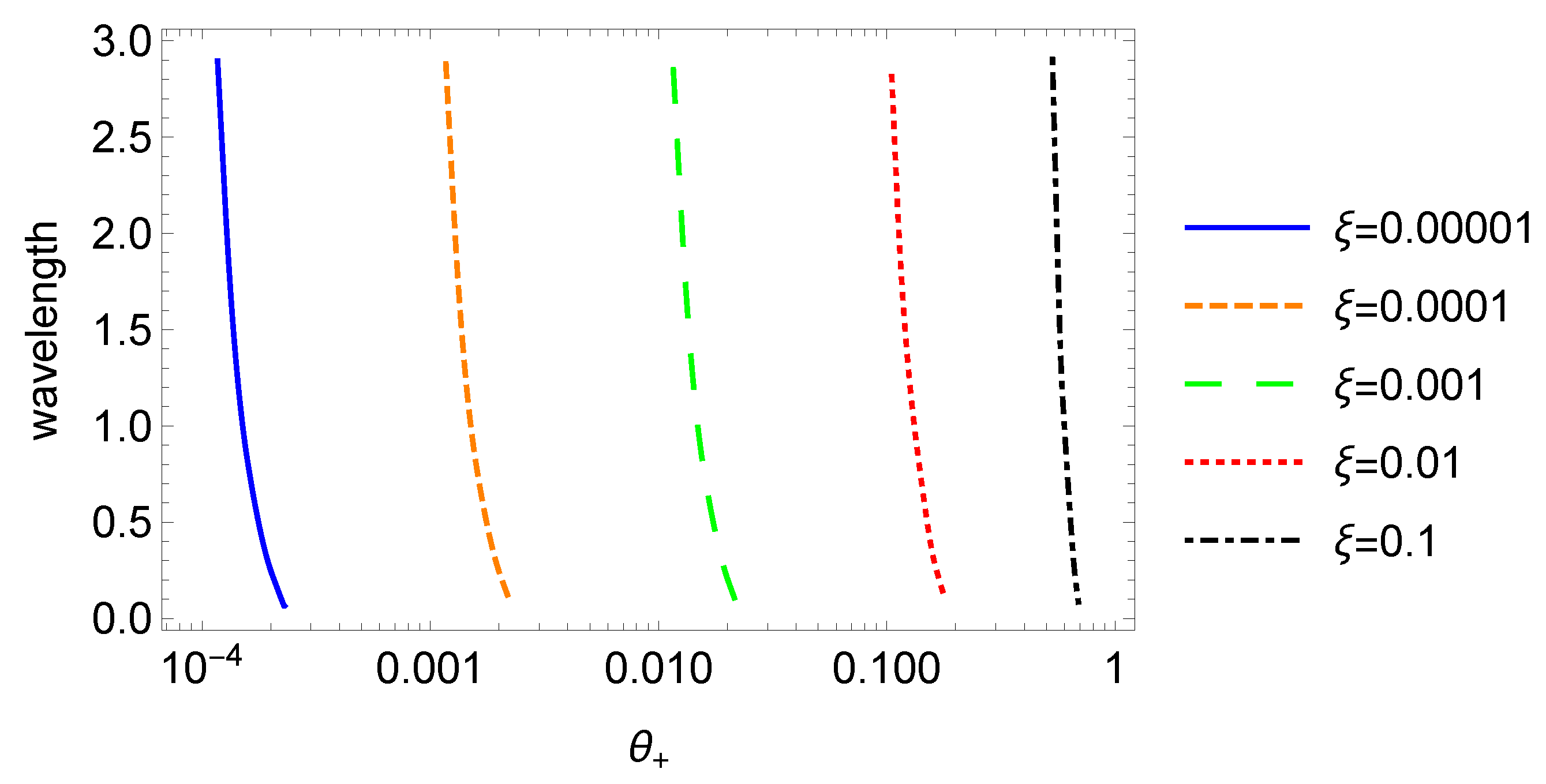
The value of plays a critical role in determining the wavelength. Figure 4 suggests that the wavelength increases with increasing and approaches the maximum value as the lower bound in is approached. It is said that, with specified , , and , the longest wavelength occurs when is at its lowest. Parker and Izumi [4], in their study of purely erosional cyclic steps, assumed that the stability of these steps is achieved when the velocity at the downstream end of hydraulic jumps equals the minimum possible value. They considered this minimum to be the threshold velocity at the onset of bed erosion. Sun and Parker [20] performed an analysis employing the same assumption that the velocity at the downstream end of hydraulic jumps is equal to the minimum possible value and found it to be in reasonable agreement with their experiments [19]. In their case, this minimum corresponds to the threshold velocity at the onset of the entrainment of sand on the bed into flowing water. The longest wavelength appears when the velocity at the downstream end of hydraulic jumps takes the minimum possible value. Their assumption that the smallest possible velocity appears at the downstream end of hydraulic jumps is synonymous with the assumption that the longest possible wavelength appears. In the case of ice steps, there is no minimum velocity at the downstream end of hydraulic jumps. We therefore assume that the longest wavelength, which is probably the most stable, appears in our analysis.
3.2. The Relationships among Parameters
The drag coefficient can be calculated by the Froude number () with Equation (24). In Appendix A, we explain another way to calculate . If the flow is laminar flow, can be calculated with the Reynolds number (). The results predicted by our analytical moodle compare with the experimental results of Yokokawa et al. [22] later. The Reynolds number detected in the experiments ranges from 228 to 2190, so the flow cannot be regarded as laminar flow. Hence, we apply to calculate the value of . The Froude number is assumed to be from 1.01 to 10, and the channel slope is assumed to be 0.05 to 0.5. The drag coefficient thus takes a range from to 0.49.
The parameter (=) is a normalized water–ice heat transfer coefficient representing the ability to transfer the heat flux from water to the ice. The value of is to , as mentioned before. It follows the range of is from to 40. The parameter (=) is the ratio of the air–water heat transfer coefficient to the water–ice heat transfer coefficient. The value of is from 1.94 to 18.15, as discussed before, and is assumed to be from 0.1 to 5 m/s. The parameter takes a value from to .
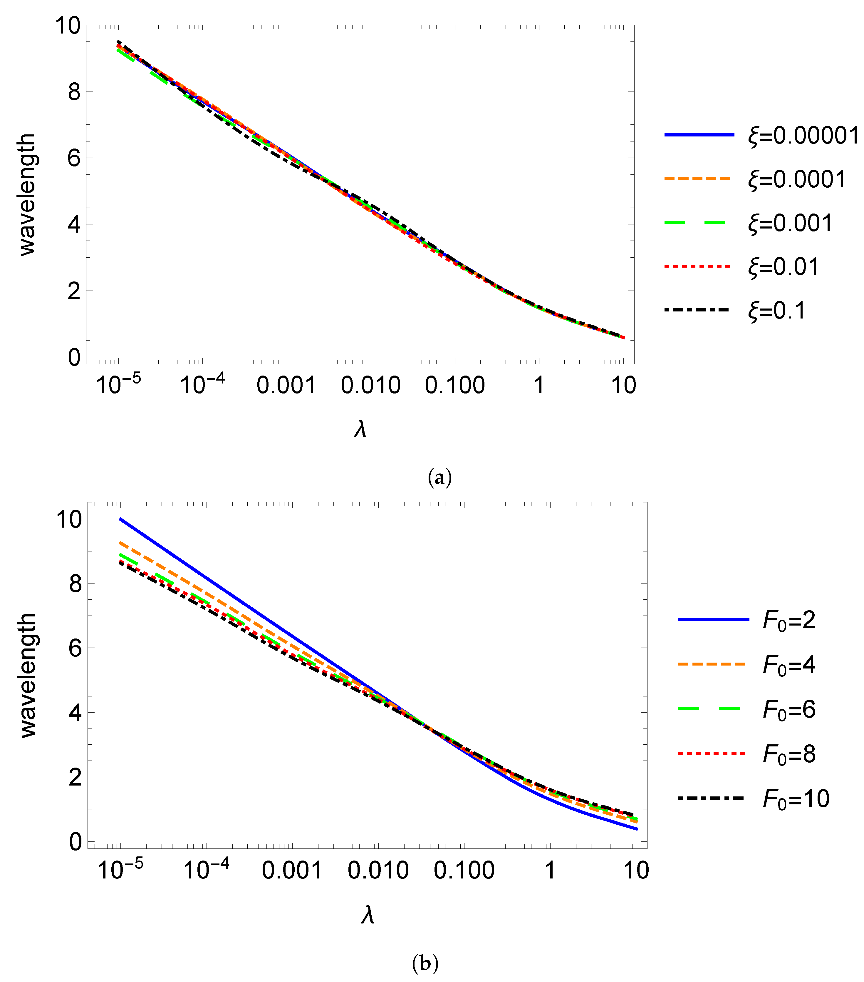
Figure 5a shows that the wavelength of cyclic steps increases with decreasing , but is nearly invariable to changes in . The former may be due to the following reasons. The amount of heat transfer across the water–ice interface per unit length reduces when the heat transfer capacity is small. In order to maintain equilibrium, a longer distance, i.e., a longer wavelength, is required to release the amount of heat transfer coming from the air–water interface. Meanwhile, the reason for the latter is not known yet, but it can be stated as follows. Keeping the water–ice heat transfer coefficient a constant, is a function only of the air–water heat transfer coefficient, denoting the air–water heat transfer capacity. According to Figure 5a, does not influence wavelength. It is found that the wavelength is more sensitive to the water–ice heat transfer capacity than the air–water heat transfer capacity.
Figure 5b suggests that the wavelength increases with when is larger than 0.034, while the wavelength decreases with increasing when is smaller than 0.034. Generally, larger values of correspond to steeper average channel slopes because is defined by Equation (24). Therefore, the wavelength decreases with increasing channel slope when the water–ice heat transfer capacity is small, while the opposite trend is observed if the capacity is large. Regarding purely erosional cyclic steps, Parker and Izumi [4] found that the wavelength increases with decreasing Froude number under normal flow conditions. Wu and Izumi [21] concluded that milder slopes facilitate the formation of longer wavelengths in the study of submarine cyclic steps formed by long-runout turbidity currents. Our study also shows the same trend when the water–ice heat transfer capacity is small. This suggests that mechanical processes also dominate in the case of ice steps when the water–ice heat transfer capacity is small, and that the same trend is observed as in the case of purely erosional and transportational cyclic steps. When the water–ice heat transfer capacity is large, on the other hand, thermodynamic processes become important, and the relationships between wavelength and show the opposite trend. Sumida et al. [24] observed an increase in the wavelength with the Froude number. Though the detailed mechanism of an increase in the wavelength with the Froude number is not yet well understood, the water–ice heat transfer capacity is expected to be large in Sumida et al.’s experiments as well.
4. Discussion
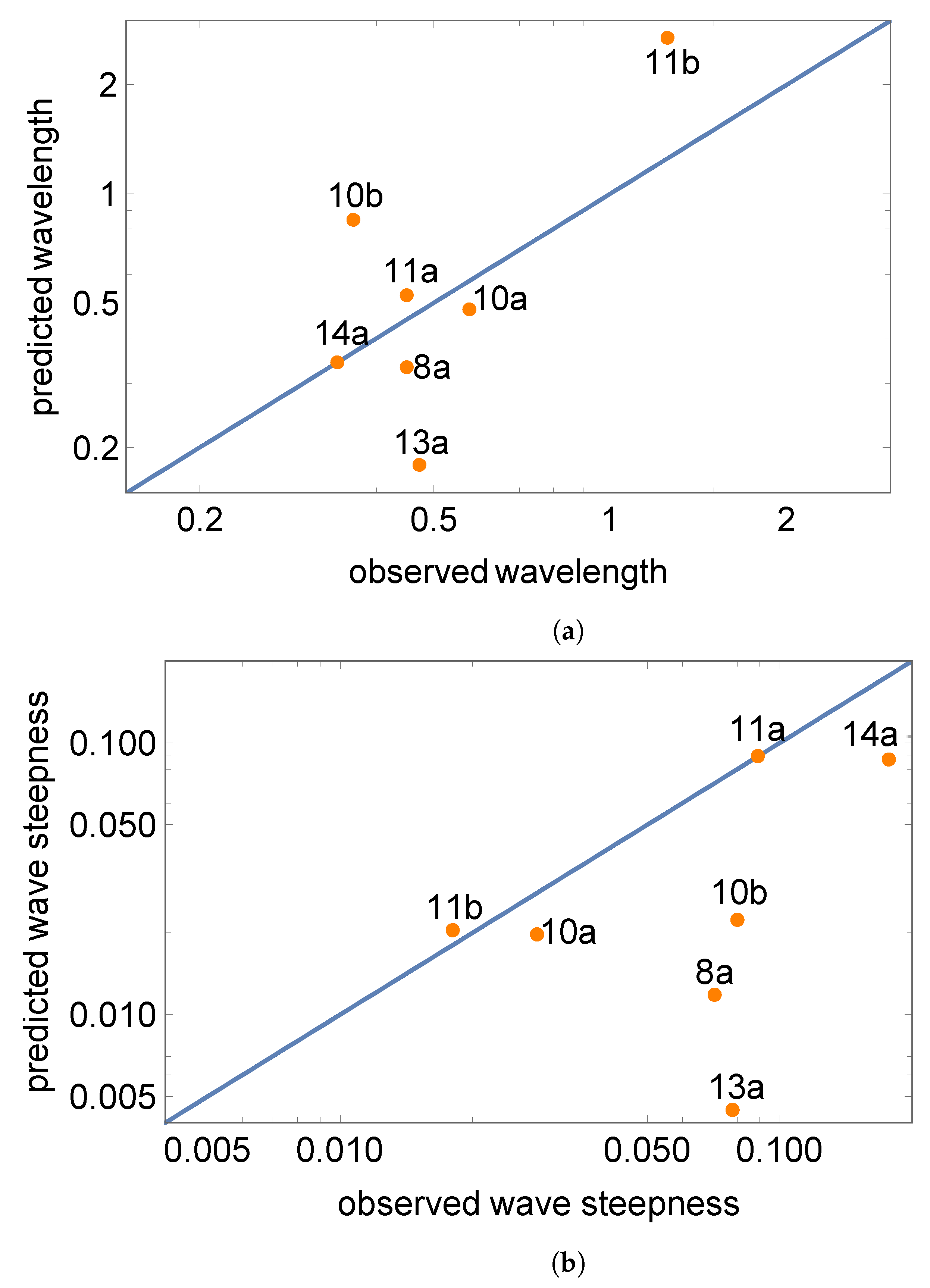
4.1. Comparison with Observed and Predicted Results
The results calculated by our model are compared with the experimental results of Yokokawa et al. [22] to validate our analysis. They performed eight experiments to reproduce the formation of cyclic steps on ice, but no bedforms were observed in one case, in which was smaller than unity. The governing equations in our model are normalized by the variables in the normal flow condition. Once we know the variables in the normal flow condition, the non-normalized results can be obtained.
Typical values for parameters are taken from the experiments, as shown in Table 1. The drag coefficient can be calculated by the Froude number (), as we discussed previously. The water temperature corresponds to and . After comparing the predicted and observed water temperature, we choose the suitable values of and to allow the predicted water temperature to agree with the observed results. The parameter is assumed as . The values of are smaller than 18.15 except for the experiment CSIM120913A. There is a possibility that the wind velocity was relatively faster in that case. The parameters and can be calculated with the aid of Equation (19) and Equation (20), respectively.
Figure 6 shows the comparisons of predicted results and observed results. The predicted wavelength is sensitive to changes in . As is defined by Equation (19), the wavelength can be influenced by the value of the dimensionless ice–water heat transfer coefficient, . This coefficient, in turn, is strongly affected by various factors, such as ice roughness and water velocity [27,28]. However, for all experimental cases, a constant value of is used in our calculations, which means that the comparisons must be considered approximate at best. It is evident that the water velocity in the CSIM120913A case is slower than in other cases, as shown in Table 1, and there is a possibility that the chosen value of is too small in this case. This notwithstanding, considering the above-noted limitations, the agreement between the observed and predicted values is acceptable except in the case of CSIM120913A.
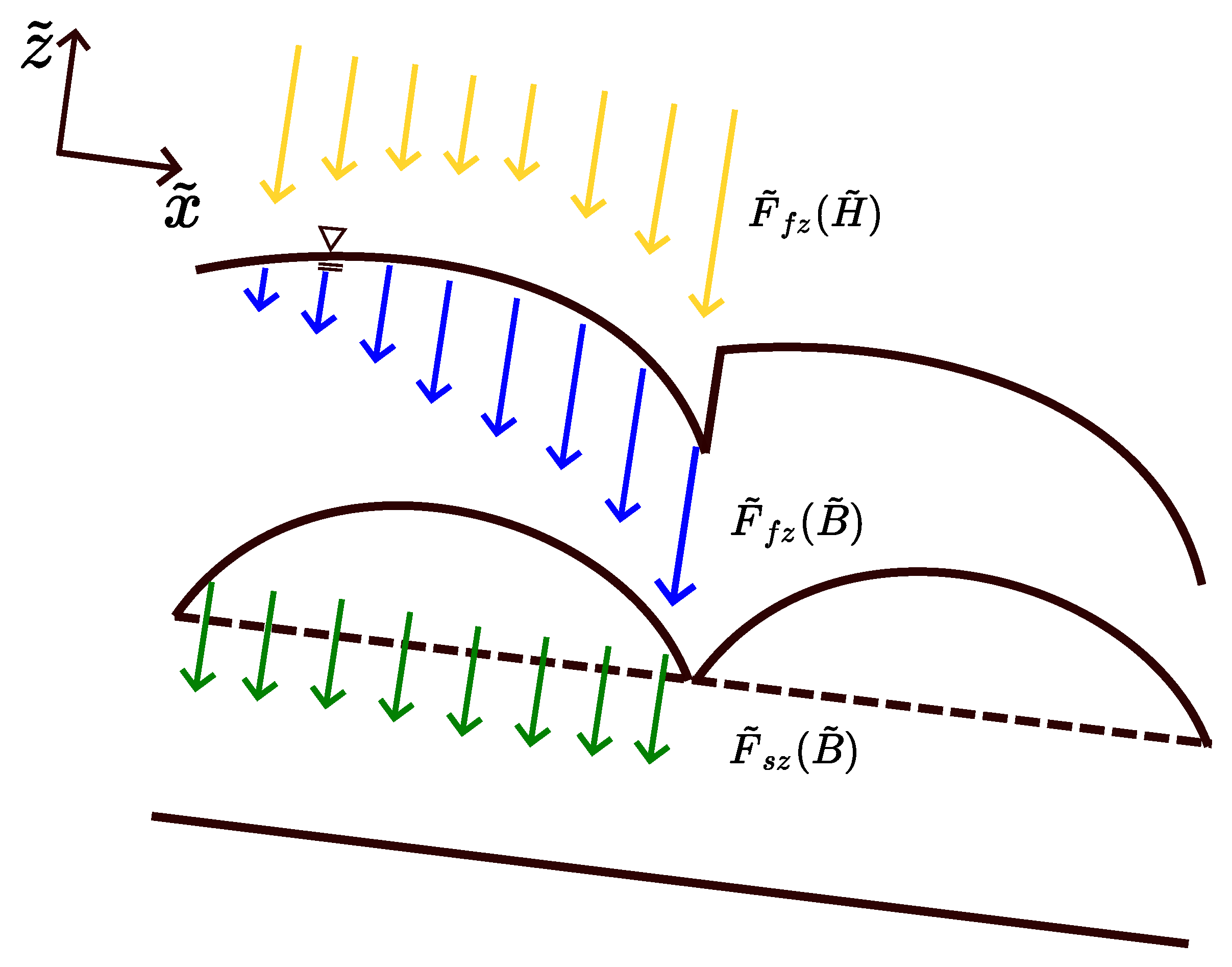
4.2. The Formation of Cyclic Steps
Figure 7 shows that the water temperature must be greater than to allow sufficient heat flux into the interface to match that going out, resulting in the melting of ice. The water temperature increases when less heat flux transfers from ice than into the water from the air. As water flow accelerates, more heat goes out from the water, and the water temperature begins to decrease. The water temperature reduces to to allow the formation of periodic cyclic steps.
The evolution of the ice surface through melting and freezing is primarily due to the difference in heat flux, as shown in Figure 7. The solidification starts after the hydraulic jump because more heat goes out from the interface than it enters. The flow continues accelerating along the streamwise direction, transferring more heat to the ice surface. The ice elevation decreases when more heat comes into the interface than goes out.
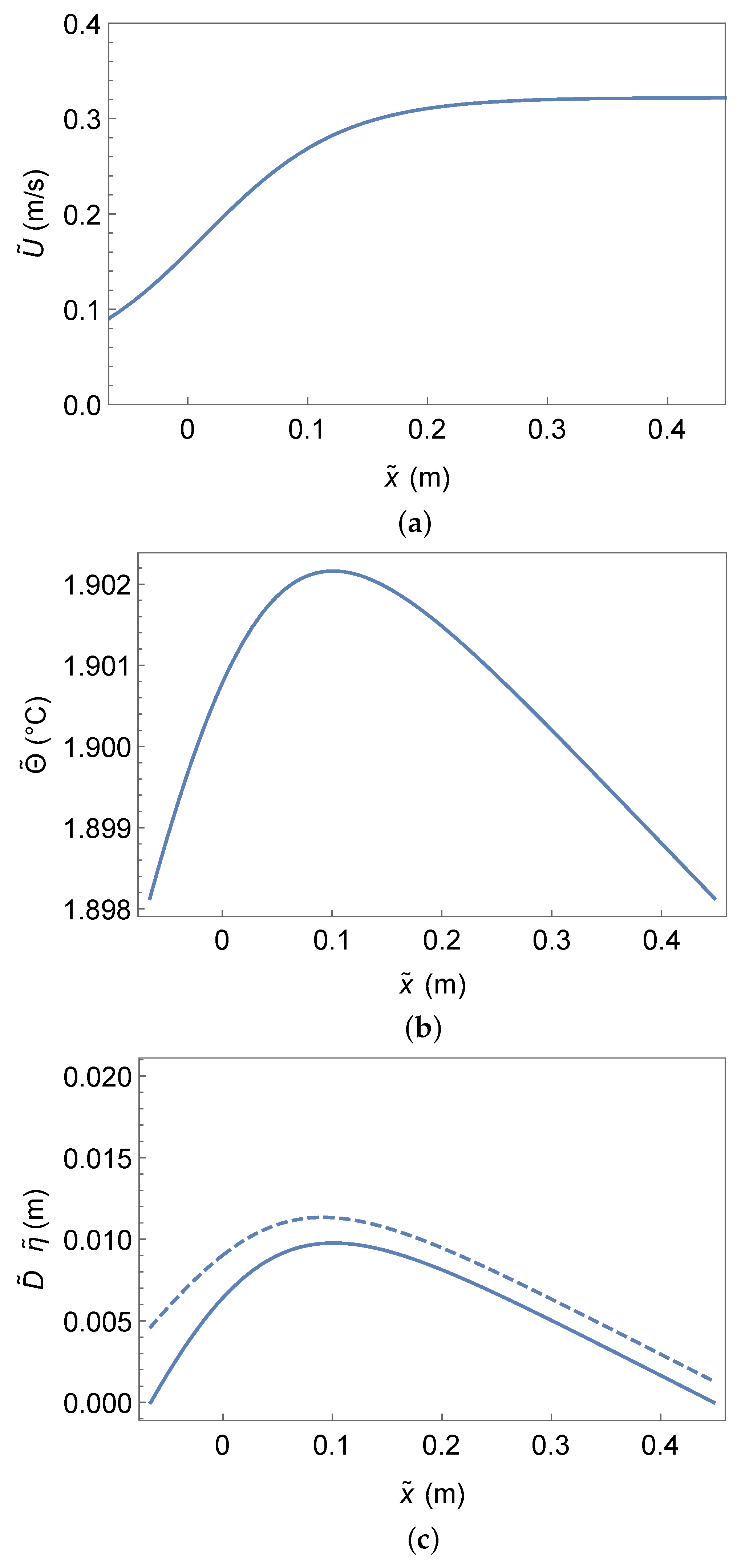
The dimensioned variations of water velocity, water temperature, and the real scales of wavelength and wave height over one step of case CSIM1209010A are in Figure 8. The flow reaches the Froude critical point at . From here, the subcritical flow becomes the supercritical flow and continues accelerating to the end of one step. Hydraulic jumps dissipate energy over a relatively short zone, and the flow transits to the subcritical regime after the hydraulic jump. The water temperature rises in the upstream of one step, since less heat goes out from the water than that coming from the air. The acceleration of water leads to more heat release, and the water temperature decreases when the heat flux from water to ice exceeds the heat flux from the air. Most cases of cyclic steps are found to satisfy the condition that the wavelength must be some orders of magnitude larger than the layer thickness. The long wave assumption is confirmed to be satisfied and the appearances of cyclic steps on ice are consistent with observations.
5. Conclusions
An analytical model is proposed to study cyclic steps on ice. To overcome previous research’s deficiency that the wavelength is difficult to determine, we apply the water temperature downstream of the hydraulic jump to calculate the wavelength. The longest wavelength is chosen for analysis. Once the parameters , , and are specified, the theory allows the prediction of migration speed, water temperature, average velocity, water surface profile, and ice elevation.
Longer wavelengths are associated with high water–ice heat transfer capacity, regardless of the air–water heat transfer ability. Moreover, for relatively weak water–ice heat transfer capacity, larger values of lead to longer wavelengths, whereas for strong water–ice heat transfer capacity, smaller results in longer wavelengths. The dimensional variables can be obtained after applying the data from the experiments of Yokokawa et al. [22]. The agreement between the predicted results of this study and the observed results is acceptable, with some limitations.
Author Contributions
Conceptualization, N.I. and Z.W.; formal analysis, N.I. and Z.W.; investigation, N.I. and Z.W.; methodology, N.I. and Z.W.; project administration, N.I.; resources, N.I.; software, Z.W.; validation, N.I. and Z.W.; supervision, N.I.; visualization, N.I. and Z.W.; writing—original draft preparation, Z.W.; writing—review and editing, N.I. All authors have read and agreed to the published version of the manuscript.
Funding
This research was funded by Hokkaido University Ambitious Doctoral Fellowship (SDGs). Grant number: JPMJFS2101.
Institutional Review Board Statement
Not applicable.
Informed Consent Statement
Not applicable.
Data Availability Statement
Not applicable.
Acknowledgments
Special thanks to all the members of the River and Watershed Laboratory for their support and helpful suggestions.
Conflicts of Interest
The authors declare no conflict of interest.
Notations
B: water bottom elevation.
: specific heat of air (=1005 J/kgk).
: specific heat capacity of water (=4184 J/kgk).
C: constant.
: constant.
: normalized heat transfer coefficient which is influenced by the wind speed.
: drag coefficient.
: dimensionless ice–water transfer coefficient.
D: flow depth.
f: migration speed of the steps in the streamwise direction.
: heat flux in flowing water in the streamwise direction .
: heat flux in flowing water in the depth direction .
: heat flux with the ice in the direction.
: Froude number associated with the normal flow in the absence of steps.
: Froude number.
g: gravity acceleration (=9.8 m/s2).
: latent heat of melting.
: bulk heat transfer coefficient of air.
: bulk heat transfer coefficient of water above ice surface (=).
H: water surface elevation.
: thermal conductivity of water.
: thermal conductivity of ice (=2.22 w/(mK)).
s: average slope.
t: time.
: air temperature.
: water temperature.
: temperature at the ice–water interface and kept to the melting point.
: temperature at the ice bottom.
: velocity component in the direction.
: friction velocity.
U: depth-averaged velocity component in the direction.
: coordinate in the streamwise.
: depth direction.
Z: ice thickness.
: non-dimensional parameter defined as the ratio of the thermal conductivity coefficient to the heat transfer coefficient in water (=).
: sum of the heat flux from the ice surface to the ice bottom and the migration speed of the ice surface in the depth direction (=).
: ice elevation.
: depth-averaged water temperature.
: normalized ice–water heat transfer coefficient (=).
: kinematic viscosity ( m2/s).
: non-dimensional parameter representing the ratio of the air–water heat transfer coefficient to the water–ice heat transfer coefficient (=)).
: air density (=1.29 kg/m3).
: density of water (= kg/m3).
: density of ice.
: degradation speed of the ice surface in the depth direction.
: bed shear stress.
: for the case of normal flow in the absence of steps.
: variables at the Froude critical point (i.e., ).
: dimensional variables.
Appendix A. Derivations of Equation and Formula
Appendix A.1. Depth-Integrated Heat Transfer Equations of Flowing Water
The heat transfer equation in flowing water is written in the form
where is the water temperature, and are the heat flux in flowing water in the and directions, respectively, and are written in the form
where is the thermal conductivity of flowing water. Equation (A1) can be rewritten in the form
where is sufficiently small compared to , and therefore, ignored hereafter. The first, second and third terms on the left hand side of the above equation are integrated from the bed () to the water surface () in the following forms, respectively:
The right hand side of Equation (A4) is integrated to be
The velocity in the depth direction at the water surface and the bed correspond to the total derivatives of the water surface and bed elevations, such that
Appendix A.2. The Calculation of the Drag Coefficient
In the normal condition, the momentum equation for the laminar flow can be rewritten into
where is the water velocity in the normal condition, and is the kinematic viscosity (). We integrate the above equation in direction to obtain
where C is a constant. When , we assume the shear stress does not exist, so we can obtain
We apply Equation (A16) into Equation (A15) and integrate Equation (A15) in the vertical direction to obtain
where is a constant. We find when and . The average water velocity in the normal condition can be expressed as
The friction velocity can be expressed as
The drag coefficient can be rewritten with the help of Equation (A17)
With the aid of Equation (A18), the above equation is in this form
where denotes Reynolds number ().
References
- Carey, K.L.; Wis, M. Observed configuration and computed roughness of the underside of river ice, St. Croix River, Wisconsin. Geol. Surv. Res. 1966, 2, B192–B198. [Google Scholar]
- Gilpin, R.R.; Hirata, T.; Cheng, K.C. Wave formation and heat transfer at an ice-water interface in the presence of a turbulent flow. Fluid Mech. 1980, 99, 619–640. [Google Scholar] [CrossRef]
- Camporeale, C.; Ridolfi, L. Ice ripple formation at large Reynolds numbers. J. Fluid Mech. 2012, 694, 225–251. [Google Scholar] [CrossRef]
- Parker, G.; Izumi, N. Purely erosional cyclic and solitary steps created by flow over a cohesive bed. J. Fluid Mech. 2000, 419, 203–238. [Google Scholar] [CrossRef]
- Lang, J.; Winsemann, J. Lateral and vertical facies relationships of bedforms deposited by aggrading supercritical flows: From cyclic steps to humpback dunes. Sediment. Geol. 2013, 296, 36–54. [Google Scholar] [CrossRef]
- Fildani, A.; Normark, W.R.; Kostic, S.; Parker, G. Channel formation by flow stripping: Large-scale scour features along the Monterey East Channel and their relation to sediment waves. Sedimentology 2006, 53, 1265–1287. [Google Scholar] [CrossRef]
- Zhong, G.; Cartigny, M.J.; Kuang, Z.; Wang, L. Cyclic steps along the south Taiwan shoal and west Penghu submarine canyons on the northeastern continental slope of the South China Sea. GSA Bull. 2015, 127, 804–824. [Google Scholar] [CrossRef]
- Paull, C.K.; Talling, P.J.; Maier, K.L.; Parsons, D.; Xu, J.; Caress, D.W.; Gwiazda, R.; Lundsten, E.M.; Anderson, K.; Barry, J.P.; et al. Powerful turbidity currents driven by dense basal layers. Nat. Commun. 2018, 9, 4114. [Google Scholar] [CrossRef]
- Ventra, D.; Cartigny, M.J.; Bijkerk, J.F.; Acikalin, S. Supercritical-flow structures on a Late Carboniferous delta front: Sedimentologic and paleoclimatic significance. Geology 2015, 43, 731–734. [Google Scholar] [CrossRef]
- Fricke, A.T.; Sheets, B.A.; Nittrouer, C.A.; Allison, M.A.; Ogston, A.S. An examination of Froude-supercritical flows and cyclic steps on a subaqueous lacustrine delta, Lake Chelan, Washington, USA. J. Sediment. Res. 2015, 85, 754–767. [Google Scholar] [CrossRef]
- Casalbore, D.; Romagnoli, C.; Bosman, A.; Chiocci, F.L. Large-scale seafloor waveforms on the flanks of insular volcanoes (Aeolian Archipelago, Italy), with inferences about their origin. Mar. Geol. 2014, 355, 318–329. [Google Scholar] [CrossRef]
- Lowe, D.G.; Arnott, R. Composition and architecture of braided and sheetflood-dominated ephemeral fluvial strata in the Cambrian–Ordovician Potsdam Group: A case example of the morphodynamics of early Phanerozoic fluvial systems and climate change. J. Sediment. Res. 2016, 86, 587–612. [Google Scholar] [CrossRef]
- Wang, J.; Plink-Bjorklund, P. Stratigraphic complexity in fluvial fans: Lower Eocene Green River Formation, Uinta Basin, USA. Basin Res. 2019, 831, 892–919. [Google Scholar] [CrossRef]
- Karlstrom, L.; Zok, A.; Manga, M. Near-surface permeability in a supraglacial drainage basin on the Llewellyn Glacier, Juneau Icefield, British Columbia. Cryosphere 2014, 8.2, 537–546. [Google Scholar] [CrossRef]
- Spiga, A.; Smith, I. Katabatic jumps in the Martian northern polar regions. Icarus 2017, 308, 197–208. [Google Scholar] [CrossRef]
- Smith, I.B.; Holt, J.W.; Spiga, A.; Howard, A.D.; Parker, G. The title of the cited article. The spiral troughs of Mars as cyclic steps. J. Geophys. Res. Planets 2013, 118, 1835–1857. [Google Scholar] [CrossRef]
- Fahnestock, M.A.; Scambos, T.A.; Shuman, C.A.; Arthern, R.J.; Winebrenner, D.P.; Kwok, R. Snow megadune fields on the East Antarctic Plateau: Extreme atmosphere-ice interaction. Geophys. Res. Lett. 2000, 27, 3719–3722. [Google Scholar] [CrossRef]
- Frezzotti, M.; Gandolfi, S.; Urbini, S. Snow megadunes in Antarctica: Sedimentary structure and genesis. J. Geophys. Res. Atmos. 2002, 107, ACL-1. [Google Scholar] [CrossRef]
- Taki, K.; Parker, G. Transportational cyclic steps created by flow over an erodible bed. part 1. experiments. J. Hydraul. Res. 2005, 143, 488–501. [Google Scholar] [CrossRef]
- Sun, T.; Parker, G. Transportationalcyclicstepscreatedbyflowoveran erodible bed. part 2. theory and numerical simulation. J. Hydraul. Res. 2005, 43, 502–514. [Google Scholar] [CrossRef]
- Wu, Z.; Izumi, N. Transportational Cyclic Steps Created by Submarine Long-Runout Turbidity Currents. Geosciences 2022, 12, 263. [Google Scholar] [CrossRef]
- Yokokawa, M.; Izumi, N.; Naito, K.; Parker, G.; Yamada, T.; Greve, R. Cyclic steps on ice. J. Geophys. Res. Earth Surf. 2016, 121, 1023–1048. [Google Scholar] [CrossRef]
- Naito, K.; Izumi, N.; Yokokawa, M.; Yamada, T. Downstream migrating steps on ice. J. Jpn. Soc. Civ. Eng. Ser. B1 (Hydraul. Eng.) 2013, 69, I1123–I1128. [Google Scholar]
- Sumida, T.; Izumi, N.; Yokokawa, M.; Yamada, T. Boundary waves formed on the ice floor due to katabatic wind. J. Jpn. Soc. Civ. Eng. Ser. B1 (Hydraul. Eng.) 2016, 72, I739–I744. [Google Scholar]
- Komori, S.; Kurose, R.; Takagaki, N.; Ohtsubo, S.; Iwano, K.; Handa, K.; Shimada, S. Sensible and latent heat transfer across the air–water interface wind-driven turbulence. In Gas Transfer at Water Surfaces; Kyoto University: Kyoto, Japan, 2010; pp. 78–89. [Google Scholar]
- Shirasawa, K.; Ingram, R.G. Currents and turbulent fluxes under the first-year sea ice in Resolute Passage, Northwest Territories, Canada. J. Mar. Syst. 1997, 11.1–11.2, 21–32. [Google Scholar] [CrossRef]
- Hamblin, P.F.; Carmack, E.C. On the rate of heat transfer between a lake and an ice sheet. Cold Reg. Sci. Technol. 1990, 18, 173–182. [Google Scholar] [CrossRef]
- Li, N.; Tuo, Y.; Deng, Y.; Li, J.; Liang, R.; An, R. Heat transfer at ice-water interface under conditions of low flow velocities. J. Hydrodyn. 2016, 28, 603–609. [Google Scholar] [CrossRef]
Figure 2.
Conceptual sketch of cyclic steps on the ice. The variable is the water surface elevation, is the water bottom, is the ice bottom.
Figure 2.
Conceptual sketch of cyclic steps on the ice. The variable is the water surface elevation, is the water bottom, is the ice bottom.

Figure 3.
Possible ranges of . The upper and lower lines with the same color denote the largest and smallest possible value for , respectively. (a) In which . (b) In which = 0.001.
Figure 3.
Possible ranges of . The upper and lower lines with the same color denote the largest and smallest possible value for , respectively. (a) In which . (b) In which = 0.001.

Figure 4.
The relationships between wavelength and . , .

Figure 5.
The relationships among wavelength and parameters. (a) . (b) .

Figure 6.
Comparison with observed and predicted results: (a) wavelength, and (b) wave steepness.

Figure 7.
Conceptual sketch of heat flux variations. Longer arrows denote more heat flux, and shorter arrows represent less heat flux. is the heat flux from air to water, is the heat flux coming into the interface from the water above, is the heat flux going out from the interface to the ice bottom.

Figure 8.
The variations of non-normalized variables over one step wavelength. (a) The variation of non-normalized velocity, (b) the variation of non-normalized average water temperature, and (c) the variation of non-normalized water surface (dashed line) and ice surface (solid line).
Figure 8.
The variations of non-normalized variables over one step wavelength. (a) The variation of non-normalized velocity, (b) the variation of non-normalized average water temperature, and (c) the variation of non-normalized water surface (dashed line) and ice surface (solid line).


Table 1.
Input parameters for the model calculation.
| Run Number | s | (m/s) | ( m) | () | () | () | |||
|---|---|---|---|---|---|---|---|---|---|
| CSIM120908A | 0.0875 | 5.5 | 0.7 | 1.52 | 0.22 | 2.05 | 2.26 | 1.58 | 3.79 |
| CSIM120910A | 0.0875 | 9.3 | 1.9 | 2.42 | 0.29 | 1.45 | 9.54 | 4.02 | 1.49 |
| CSIM120910B | 0.0875 | 5.7 | 0.7 | 3.17 | 0.40 | 1.65 | 8.59 | 6.89 | 0.87 |
| CSIM120911A | 0.3640 | 5.5 | 0.5 | 4.31 | 0.62 | 2.12 | 2.69 | 3.06 | 1.96 |
| CSIM120911B | 0.0875 | 5.2 | 0.2 | 2.89 | 0.68 | 5.70 | 2.10 | 5.73 | 1.05 |
| CSIM120913A | 0.0875 | 5.3 | 2.2 | 1.11 | 0.17 | 2.29 | 5.82 | 0.84 | 7.10 |
| CSIM120914A | 0.3640 | 5.4 | 0.5 | 4.37 | 0.48 | 1.25 | 2.85 | 3.15 | 1.91 |
Disclaimer/Publisher’s Note: The statements, opinions and data contained in all publications are solely those of the individual author(s) and contributor(s) and not of MDPI and/or the editor(s). MDPI and/or the editor(s) disclaim responsibility for any injury to people or property resulting from any ideas, methods, instructions or products referred to in the content. |
© 2023 by the authors. Licensee MDPI, Basel, Switzerland. This article is an open access article distributed under the terms and conditions of the Creative Commons Attribution (CC BY) license (https://creativecommons.org/licenses/by/4.0/).
Share and Cite
MDPI and ACS Style
Wu, Z.; Izumi, N. Cyclic Steps Created by Flowing Water on Ice Surface. Geosciences 2023, 13, 128. https://doi.org/10.3390/geosciences13050128
AMA Style
Wu Z, Izumi N. Cyclic Steps Created by Flowing Water on Ice Surface. Geosciences. 2023; 13(5):128. https://doi.org/10.3390/geosciences13050128
Chicago/Turabian StyleWu, Zhuyuan, and Norihiro Izumi. 2023. "Cyclic Steps Created by Flowing Water on Ice Surface" Geosciences 13, no. 5: 128. https://doi.org/10.3390/geosciences13050128
Note that from the first issue of 2016, this journal uses article numbers instead of page numbers. See further details here.