Article

2D FEM Numerical Prediction of Local Seismic Effects at San Salvador Municipality (El Salvador) Induced by 2001 Earthquakes

by
Chiara Faraone
1,*,
Serena Caravaggio
1,
José Alexander Chávez
2,
Luis Alfonso Castillo Ramos
1,3,
Mario Luigi Rainone
4 and
Giovanna Vessia
1
1
Department of Engineering and Geology (INGEO), University “G. d’Annunzio” in Chieti-Pescara, 66100 Chieti, Italy
2
Planning Office of the Metropolitan Area of San Salvador (OPAMSS), San Salvador 01101, El Salvador
3
Department of Geophysics, University of El Salvador, San Salvador 01101, El Salvador
4
Department of Psychological, Humanistic and Territorial Sciences (DiSPuTer), University “G. d’Annunzio” in Chieti-Pescara, 66100 Chieti, Italy
*
Author to whom correspondence should be addressed.
Geosciences 2023, 13(4), 116; https://doi.org/10.3390/geosciences13040116
Submission received: 28 February 2023 / Revised: 5 April 2023 / Accepted: 7 April 2023 / Published: 13 April 2023
(This article belongs to the Special Issue Natural Hazards and Geological Risks in Subduction Zones)

Abstract

:
San Salvador Metropolitan Area (MASS) is an urbanized territory in the country of El Salvador, located between the San Salvador volcano and the Ilopango caldera, in a sub-flat area called “Valle de las Hamacas” (Valley of the Hammocks). The high seismicity of this area is due to the subduction zone of the Cocos plate that causes strong seismic events such as the earthquakes that occurred on 13 January (7.6 Mw) and 13 February 2001 (6.6 Mw). As part of the international cooperation project between Italy (AICS) and El Salvador University, the CASTES project focussed on natural hazards in the territory of El Salvador was launched. Therefore, 2D simulations are carried out along two sections to evaluate the Local Seismic Response (LSR) in the Southeast part of MASS territory. Results show spatially variable amplifications (from 3 to 6.5) in the period ranging 0.1–0.7 s and evidence of lateral FA variations that can be calculated only through 2D numerical analyses. Two amplified periods are recognised, 0.1–0.5 s and 0.4–0.8 s, due to the presence of two types of subsoil volcanic deposits: the shallow and soft Tierra Blanca deposits and the deeper and stiffer Volcanic ash and Tuff.

1. Introduction

Numerical prediction of local seismic effects in urban areas is performed worldwide through 1D, 2D, and 3D simulations based on methods such as Finite Element (FE) [1,2,3,4,5,6], Finite Difference (FD) [7,8,9,10] and Spectral Element (SE) [11,12,13] and the references herein. This approach aims at modelling the complex geo-morphological and litho-technical subsoil characters to predict the effect at the surface of the seismic wave propagation, in terms of spectral acceleration, velocity and displacements, and amplification factors and functions [14] and to evaluate the influence of these effects on damage over large areas [15]. These studies are needed to draw maps of seismic shaking effects (in terms of amplitude, frequency content, and duration) throughout the urbanized areas, leading urban planning to improve the resilience of human communities [16]. To this end, a higher education and research project named CASTES (Establecer y desarrollar la carrera de Licenciatura en Ciencias de la Tierra con énfasis en Geología en la Universidad de El Salvador: https://castes.agronomia.ues.edu.sv/ accessed on 11 January 2023) has been developing in El Salvador since the year 2020 with the financial support of AICS (Italian Agency for Development and Cooperation) and the joint scientific coordination of the University of Palermo and Chieti-Pescara. Among the research objectives are seismic hazard assessment and the evaluation of the co-seismic effects at urban sites to increase the resilience of people living in the city centres affected by large earthquakes. This is the case of the large municipality of San Salvador, also known as MASS (Metropolitan Area of San Salvador), which has been hit and damaged by the seismic events on 13 January (Mw 7.6) and 13 February 2001 (Mw 6.6).
The buildings in the central MASS territory are masonry, reinforced concrete, and reinforced brick masonry (named mixto) dwellings. Furthermore, làmina (structural system composed of wood or metal frames), adobe and baraques [17] can be found on the outskirts of the municipal area.
Accordingly, in the central area of MASS, buildings commonly have a number of storeys ranging between three and seven, while on the outskirts, buildings are lower (two floors). In the western area, there are high buildings whose number of floors vary between nine and 22 [18].
The main objective of the present study is to evaluate the local seismic response (LSR) at the MASS site to compare with the damage that occurred after the strong earthquakes of 2001 for shedding light on the role of the geological formations outcropping at MASS that generated seismic differentiated amplifications and damage. To this end, the contribution of the Tierra Blanca (TB) deposits to surficial amplifications has been investigated through two-dimensional numerical analyses (2D) of LSR performed with the LSR2D Finite Element code [19]. As input motions, the two horizontal components (EW and NS) of the mainshocks related to the 13 January and 13 February 2001 earthquakes have been used.
Hereinafter, Section 2 summarises the study on LSR in the San Salvador municipality area; Section 3 and Section 4 describe the tectonic, geological features, and historical seismicity of El Salvador and the MASS territory, respectively. Section 5 presents the adopted methodology for the numerical analyses and introduces the studied subsoil sections and their numerical models. In Section 6 the results are illustrated and in Section 7 they are discussed by comparing 1D and 2D amplified periods in these almost flat stratigraphic conditions.

2. State of the Art of Microzonation Studies in Metropolitan Area of San Salvador

Numerous studies have evaluated the local site effects in the aftermath of the numerous strong seismic events in the El Salvador region [20], particularly in the metropolitan area of its capital, San Salvador. However, they do not always provide consistent results probably due to the complex geological setting of the territory and the scarcity of available subsurface data [21].
The first seismic zonation study in MASS was proposed by [22]. The author presents a map of the thickness of the TB deposits that points out its strict relationship with the intensity of the seismic shaking. It is witnessed by the larger damage caused by the earthquake of 3 May 1965, where higher thicknesses were detected. Just four years later, in the work by [23], factors for increasing soil acceleration according to the thickness of the (TB) deposits were defined in the MASS. These studies confirmed the direct relationship between the increase in acceleration, the thickness of the aforementioned deposits and the depth of the bedrock for far-field earthquakes.
Another proposal for microzonation of this metropolitan area, based on the observation of microtremors, was made in 1985 by [24]. The author drew a map divided into six microzones, each defined by a certain range of amplification factors (from one to three) corresponding to a period of 0.5 s.
In 1988 the first seismic microzonation map was drawn up by [25] in the south-central part of the MASS. The authors, after collecting and ordering data from subsoil investigations, geophysical testing, and laboratory geotechnical tests, performed seismic response analyses using the recordings of the strong motion of 10 October 1986 (Mw 5.7) as the seismic input. This map identifies (1) Zone 1 with a thickness of 65 m of lava flows, subdivided, in turn, into two sub-zones: 1A where lava flows outcrop or are located within the first 5 m from the surface, and 1B where the lava flows are located from 5 to 35 m depth; and (2) Zone 2 with a total thickness of 35 m of lava flows. Concerning the 1986 earthquake, the greatest damage occurred in the area characterized by an amplified period of 0.2–0.5 s and the TB deposits reached 15–25 m in thickness.
A geotechnical approach, performed by Aguilar [26], allowed the definition of the fundamental periods for six different zones within the MASS (from 0.095 to 0.89 s), through the correlation of geotechnical parameters (such as the number of blows) of a standard penetration test and a dynamic parameters of refraction seismic test with the thicknesses of the TB, and the depth of the bedrock [22].
Another work using a geotechnical approach to identify the fundamental periods of different lithological columns is the one carried out by [27]. The authors produce a paper with iso-periodic curves stating that the soil vibration periods within MASS fluctuate between 0.1 and 1.2 s and their heterogeneity is due to the variation in depth of the stiff layer (the lava one). The most urbanized portion falls within the zone with characteristic periods ranging between 0.4 and 0.6 s.
In [28], one-dimensional viscous-elastic numerical analyses were performed in the municipality of San Salvador with the input motion taken from destructive earthquakes generated from both the upper crust and subduction zones. Results were drawn in terms of response spectra and transfer functions (whose values were lower than 10 in the range of 0.1–1.0 s). These authors [28] argued that the induced amplification based on transfer functions calculation is due to the strong impedance contrast between the surface loose deposits and the lava rocks at the bedrock.
The highest amplifications (about 3) are visible at the slopes of the Ilopango caldera where the thickness of the TB deposits becomes important (about 50 m).
Another study that evaluated the seismic response at different points in the MASS using seismic noise measurements and strong motion recordings at geologically known sites is reported in [29]. The authors found that the lowest periods are those near the volcano San Salvador (0.2 s) while the highest ones are found at the slopes of the caldera of Ilopango (0.47 s) where the thickness of the sediments of the TB exceeds 25 m.
Burgos et al. [30] show a study of the microtremor data in which the fundamental vibration periods for each point of measurement have been evaluated from the thickness of TB: where it varies between 3 and 6 m, the amplified period is 0.28 s and where the thickness is higher than 25 m, longer amplified periods are observed (also confirmed by [31]).
Based on the Nakamura Horizontal to Vertical Spectral Ratio (HVSR) technique, the work presented by [32] established the values of the amplified frequencies, wave velocities, and TB thickness in 10 areas of the San Salvador metropolitan territory.
Salazar [31] assessed the local seismic response in Metropolitan Area of San Salvador made by equivalent linear numerical analysis (with the “SHAKE2000” software) on models calibrated through empirical methods (Borcherdt Methods and Nakamura technique). The authors clarify that the fundamental period of the subsoil increases as the thickness of poorly consolidated sediments increases. In general, the low periods were found near the volcano San Salvador. Later, Kattan [21] shows a preliminary map of five areas susceptible to local amplification in the MASS, based on the thicknesses detected by [25] each with a specific range of periods. Most of the town is set on soils with periods between 0.2–0.5 s and 0.4–0.9 s corresponding to amplification values of 2.2 and 2.5, respectively.
Although numerous LSR have been performed over time in MASS, none of them reconstructed 2D sections of MASS subsoil and carried out equivalent linear numerical analyses. The novelty of this study, then, consists in carrying out 2D numerical simulations along two vertical sections within MASS area where damages occurred during the January 2001 earthquake.
The final aim is reconstructing the geometrical heterogeneity of the subsoil and highlighting the sharp variations of the amplification factors influencing the differentiated damages observed in the studied municipality territory.

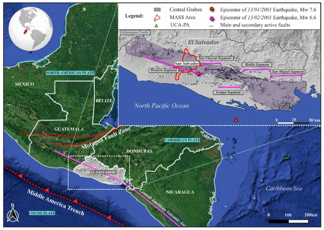
3. Geographical, Tectonic, and Geological Setting of the El Salvador Region

El Salvador country is located in the Central American Volcanic Arc (CAVA), which extends from Guatemala to Costa Rica along the active Pacific margin and ends to the north in a diffuse triple junction among the Cocos, Caribbean, and North American plates (Figure 1) [33,34,35,36].
The CAVA accommodates the fault system in El Salvador region, named El Salvador Fault Zone (ESFZ), that crosses the country from east to west [39] connecting with the Jalpatagua Fault [37,40,41]. The ESFZ is 150 km long and 20 km wide of distributed strike-slip faulting. The ESFZ is divided into five sectors (see the inset in Figure 1), which are named, from west to east: Western Segment, San Vicente Segment, Lempa Segment, Berlin Segment, and San Miguel Segment [39].
El Salvador is affected by earthquakes from two main sources of seismicity: (1) the Middle America Trench subduction zone, generating large magnitude earthquakes (>7 Mw); (2) the upper crustal volcanic arc deformation zone, generating moderate to large magnitude earthquakes (≤7 Mw).
The first one, at depths ranging between 50 to 150 km, is located along the Wadati-Benioff subduction plane. The 13 January 2001 earthquake was generated from this latter source.
The second source of seismicity is characterized by upper crustal earthquakes that are prevalently of tectonic origin [42,43] (and are generated in the “volcanic chain” area) and connected to a right-lateral shear zone that is related to the oblique component of the collision of the Cocos and Caribbean plates [34].
Earthquakes associated with the volcanic chain have a magnitude that rarely exceeds 6.5 [44] but they have shallow focuses (hypocentres at depths up to 30 km). The 13 February 2001 earthquake was generated by this seismic source.
In Table 1 several strong earthquakes that occurred in El Salvador during the past century are listed according to their sources: A for the Volcanic chain and B for the subduction zone.
The morpho-tectonic character of El Salvador country controls the sedimentation and geological features of the whole territory. The geological units almost entirely consist of volcanic rocks (andesites, basalts, rhyolites, lavas, and pyroclastic rocks), whose age decreases spatially from north to south. A portion of less than 5% of the territory to the north, instead, is covered by ancient sedimentary rocks of the Jurassic–Cretaceous ages. Finally, alluvial deposits crop out alongside the coast of the Salvadoran territory [22].

3.1. Historical Seismicity of the Metropolitan Area of San Salvador (MASS)

The capital city of San Salvador is, amongst Latin American cities, the most frequently damaged and destroyed by earthquakes: at least twelve times since 1576 [45].
The most damaging historic earthquakes are listed in Table 2, although they vary in their destructiveness (more destructive quakes in yellow in Table 2): (1) on 16 April 1854 (the largest of the crustal earthquakes) an event of 6.6 estimated magnitude occurred: it caused large destruction in San Salvador such that the capital was relocated to Santa Tecla for a period of five years; (2) on 8 June 1917, when two almost consecutive events with (6.4 and 6.3 Ms) occurred followed by an eruption half an hour later; (3) on 10 October 1986; the magnitude of this earthquake was not that high (5.7 Ms) but occurred at a shallow depth directly beneath San Salvador where the felt intensity IMM was as high as IX, causing about 1500 casualties and making over 100,000 homeless [45,46,47].

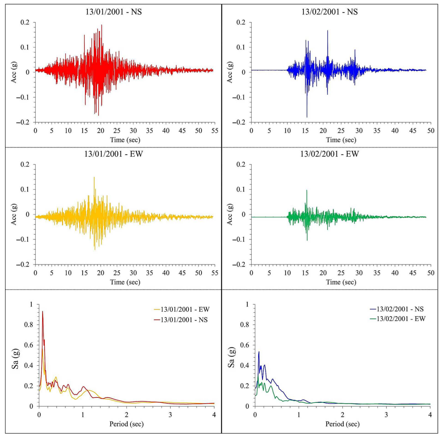
3.2. The Two Strong 2001 Earthquakes

In 2001, El Salvador was hit by two major earthquakes (the inset in Figure 1): the first, a normal-faulting event in the subduction zone, that occurred on 13 January 2001 (7.6 Mw): the epicentre was located 110 km SE of San Salvador capital city (Costa del Sol, 13.0498° N and −88.660° W) at a focal depth of about 60 km. The second occurred on 13 February 2001 (6.6 Mw), a strike-slip crustal earthquake whose epicentre was located near the city of San Vicente (13.621° N, 88.856° W) in the weakness zone of the volcanic axis [47], at 30 km east of San Salvador capital city [50] and a focal depth of 9 km [35].
Concerning the first seismic event, the mainshock was followed by a large number of aftershocks (more than 5000) that were recorded for over 6 weeks.
The time histories of the mainshock recorded motions along N–S and E–W directions at Panchimalco (PA) in 2001 show that the duration of strong shaking is approximately 50 s with a predominant period of about 0.08 s for both directions, suggesting higher energy contents at higher frequencies (about 13 Hz).
The 13 February 2001 earthquake was different from the 13 January one because it was a strike–slip event that took place inside the upper continental plate. The mainshock was followed by aftershocks that covered an area of 300 km2. The strong motion duration was 30 s and the predominant period was equal to 0.09–0.22 s for both components.
However, the 13 January and 13 February 2001 caused heavy damage, widespread across the country: 844 and 315 casualties, respectively. Table 3 reports the victims and the disruptions caused by the two strong seismic events in the MASS [44]. These earthquakes caused damage as large as VII-VIII IMM in the San Salvador area [51].
Local seismic effects were suffered at MASS where large areas are covered by loose and unconsolidated deposits of the quaternary unit of TB deposits with poor mechanical characteristics [20] and rather low values of the shear wave velocity, which likely influenced the amplitude and frequency contents of the seismic shaking. Even in San Salvador, extensive damage was observed in shanty dwellings.
The damages to structures and dwellings were described by [44]. The authors report the cumulative percentage damage ratio for the two strong 2001 earthquakes as the ratio between the collapsed houses and total houses. The MASS suffered a damage ratio between 5% and 25%. The Figure 2 shows the areal distribution of the number of floors within MASS. In the study area (see black rectangle in Figure 2) the number of stories in each dwelling vary between three and seven.

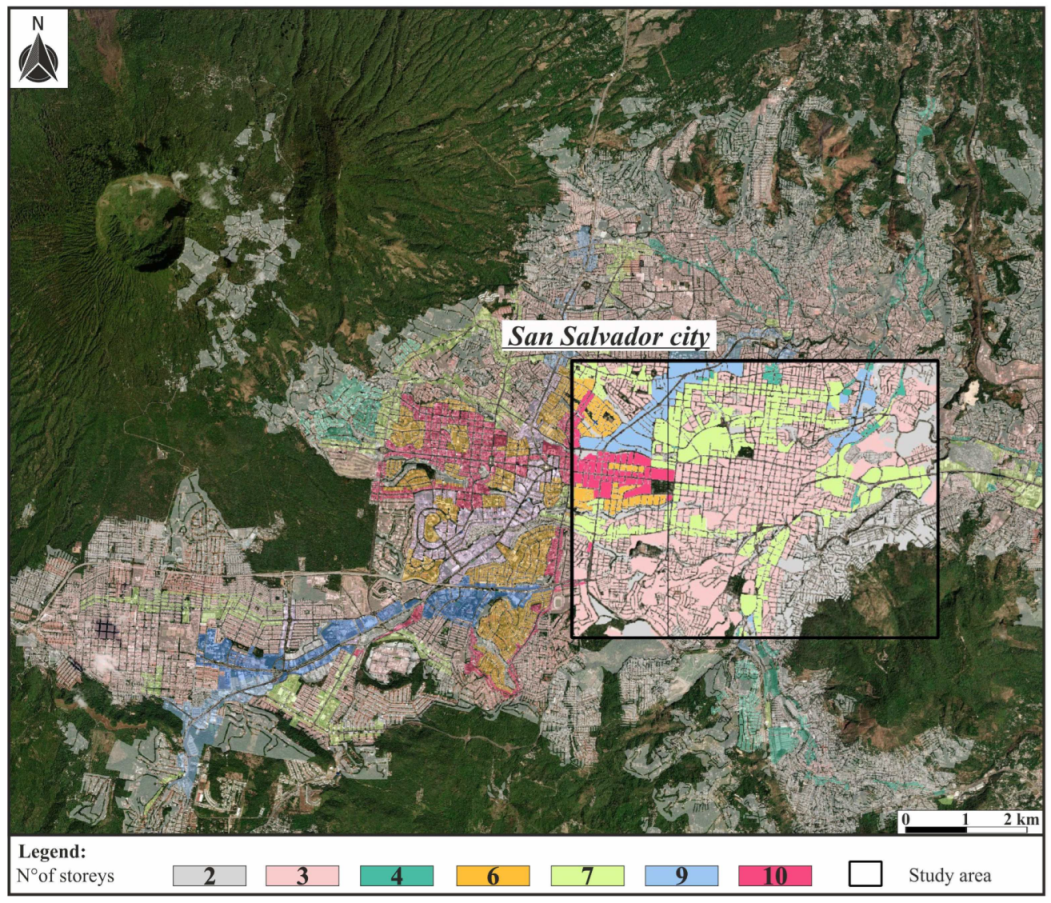
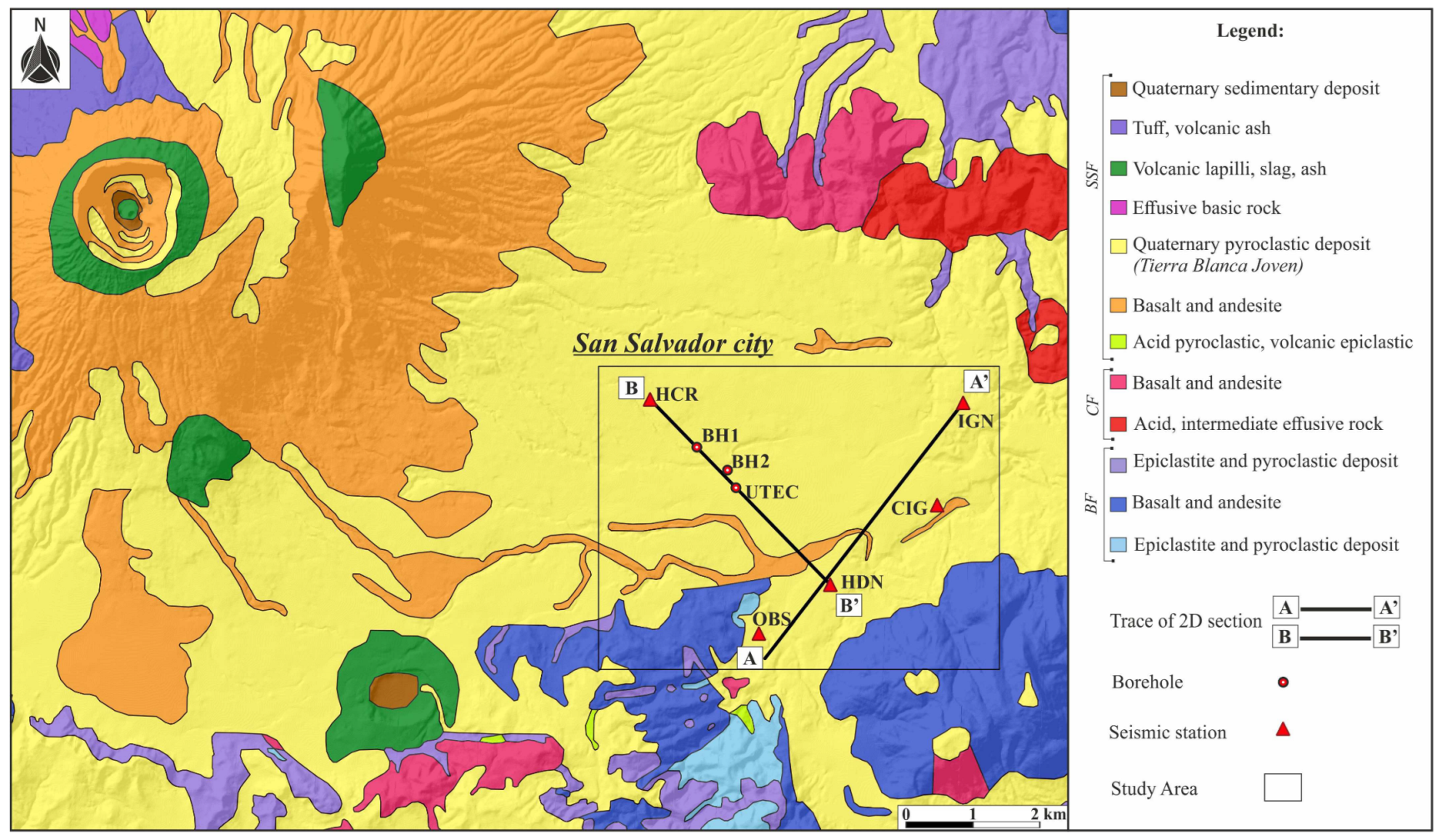
4. Geological, Seismological, and Litho-Technical Features of Metropolitan Area of San Salvador

The Department of San Salvador is located within the Central Graben and extends to an area of 609.9 km2 straddling two active volcanoes: the San Salvador to the North-West and the Ilopango to the South-East.
In the MASS territory, several right-lateral strike-slip faults are present that bound the subsided block of the Central Graben against the uplifted and southward tilted block of the Cordillera del Balsamo.
The horst geological structure of the southern margin of the central Graben consists of the ancient Bálsamo Volcanic Formation (Late Miocene-Pliocene), made up of andesitic and basaltic lavas with interbedded tuff and ignimbrite. This formation underlays the Cuscatlán Geological Formation (Plio-Pleistocenic) consisting of acid ignimbrites with basic lavas interbedded [21].
The Bálsamo Formation is the oldest lithostratigraphic unit formed of andesite lavas, tuffs, and epiclastic volcanic breccias/conglomerates representing remnants of andesite stratovolcanoes. This formation is the geological substrate in the MASS area.
Most of the whole urban territory includes basalt/andesite stratovolcano products associated with the evolution of the central Graben [52].
In the MASS area, the TB Volcanic Deposits outcrop (belonging to the San Salvador Formation datedto Late Pleistocene-Holocene), composed of dalacitic pumice ash composed of acid and epiclastic pyroclastic deposits, covers most of the upper part of the San Salvador metropolitan area [53] (Figure 3).
These deposits can be classified as sandy silt or silty sand [55] and along the depth, they can be divided into four main units, that are, from the oldest to the youngest, TB4, TB3, TB2 (Tobas superiores) and TBJ (Tierra Blanca Joven). Each of them is separated by a brownish-reddish palaeosoil a few meters thick [56].
The most frequently outcropping soil is the TBJ unit resulting from the last explosive eruption of Ilopango [57]. The TBJ shows a thickness varying from a few meters (0–3 m) up to tens of meters (>25 m) within the MASS area, especially along the slopes of volcanic structures [58].
Kattan [21] described the deposits of TBJ and TB (poorly consolidated) with shear seismic wave velocities between 150–450 m/s and compression seismic wave velocities VP varying in the range of 300–1000 m/s, and lavas with a shear seismic wave velocity of about 2000 m/s and compression seismic wave velocity in the range between 2600–3200 m/s (assumed as the seismic bedrock).
In general, the thickness of the unconsolidated sediments in the MASS territory is variable and therefore plays a fundamental role in seismic amplification in the range of periods of the engineering interest (0.1–1.0 s).

5. 2D Local Seismic Response in MASS

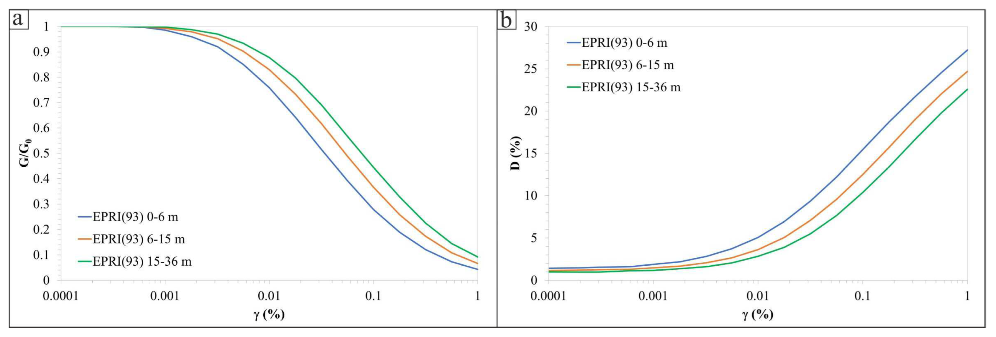
5.1. Equivalent Linear Analyses for Finite Element Simulations

Two-dimensional numerical analyses have been performed through an equivalent linear approach in the time domain solution of seismic shear wave propagation SH. We used LSR2D code, by [19]. It implements the finite element method, FEM, that allows calculating stresses and deformations, under total stress conditions (meaning that the whole modelled domain is assumed to be fully saturated), induced by the 2D propagation of horizontal shear waves SH and compressional waves P through soils and rock formations from a horizontal non-rigid rocky bedrock up to the surface. The input motion has been applied at the bedrock (at the bottom of the model) by deconvolving the recorded horizontal component of the motion at the surface (at the seismic station). At the bottom of the model, a compliant base condition is assumed whose properties are provided through the shear wave velocity of the bedrock. The dynamic motion equation solved by the FEM code at each node of the mesh grid follows:
M u ¨ + C e + C b u ˙ + K u = M I x u b , x ¨ t M I y u b , y ¨ t + F f f ( t )
where: M = the global mass matrix of the equation system, C e = global damping matrix of the finite element node system; C b = global damping matrix of the viscous dampers at the bottom of the mesh; K = global stiffness matrix of the equation system; u ¨ = global acceleration; vector, u ˙ = global velocity vector and u = global displacement vector of the equation system; I x = the drag global vector along horizontal direction; I y = the drag global vector along vertical direction; u ¨ b , x , y = horizontal and vertical components of the input acceleration vector; F f f ( t ) = dynamic forces that simulate the free field conditions at the vertical edges of the modelled domain.
Through the equivalent linear constitutive model, the non-linear and non-elastic behaviour of soils under seismic solicitations is represented through the reduction curve of the shear modulus G as the shear strain amplitude increases γ: it is updated at each time step of the analysis according to the γ value induced by the input solicitation [59]. Accordingly, to take into account the damping effects of the cyclic degradation, the damping curve D(γ) is used to update the damping values to the shear strain level. Several curves of G/G0(γ) and D(γ) from the literature are available and often used for such numerical simulations on soils according to some physical parameters.
The global damping matrix, C e is obtained by assembling the finite element damping value through a classical Rayleigh scheme. For each element I, the damping can be written as:
C i = α R , i M i + β R , i K i
where α R , i and β R , i are the Rayleigh coefficients and Mi and Ki are the mass and stiffness matrices of each finite element, respectively. This calculation has been internally performed by LSR2D code that is used hereinafter.
The whole domain has been divided into triangular elements whose maximum side dimension depends on the cut-off frequency, that is the maximum propagated frequency fmax. Commonly, for far-field sites, fmax = 20 Hz is assigned. Then, the following rule has been adopted for the maximum element side dimension h, to avoid the aliasing phenomenon in the numerical simulation [60]:
h = V S 6 ÷ 8 · f m a x
where VS is the shear wave velocity and fmax is the maximum frequency value that is numerically propagated from the bottom to the top of the model.
The input motion is applied at the bottom of the model domain, and results have been reported in terms of acceleration spectral responses and the acceleration amplification function. This latter is the ratio, in the period/frequency domain, between the output response spectrum at a point on the upper surface of the modelled domain and the input response spectrum applied at the bottom of the model, representing the bedrock line. Furthermore, Amplification Factors have been calculated, according to the following expression:
F A = T 1 T 2 S A o u t T d T T 1 T 2 S A i n T d T
where SA is the acceleration spectrum calculated as output on the surface (SAout) and applied as the input (SAin) at the bottom of the model; T1 and T2 are the bounds of the period ranges considered in this study: 0.1–0.5 s, 0.4–0.8 s, and 0.7–1.1 s [61].
Finally, lateral boundary conditions have been adopted to simulate the absorption of the wave-associated energy by the semi-infinite domain according to these equations:
F x = ρ V P u ˙ x m u ˙ x f f A
F y = ρ V S u ˙ y m u ˙ y f f A
where: 𝜌 = soil mass density of the soil; 𝑉P: P wave velocity of the soil; 𝑉S: S wave velocity of the soil; 𝐴: the influence area of the damping node; u ˙ y m : node velocity in x-direction; u ˙ y m : node velocity in y-direction; u ˙ x f f : node velocity of the free field column in x direction; u ˙ y f f : node velocity of the free field column in y direction.

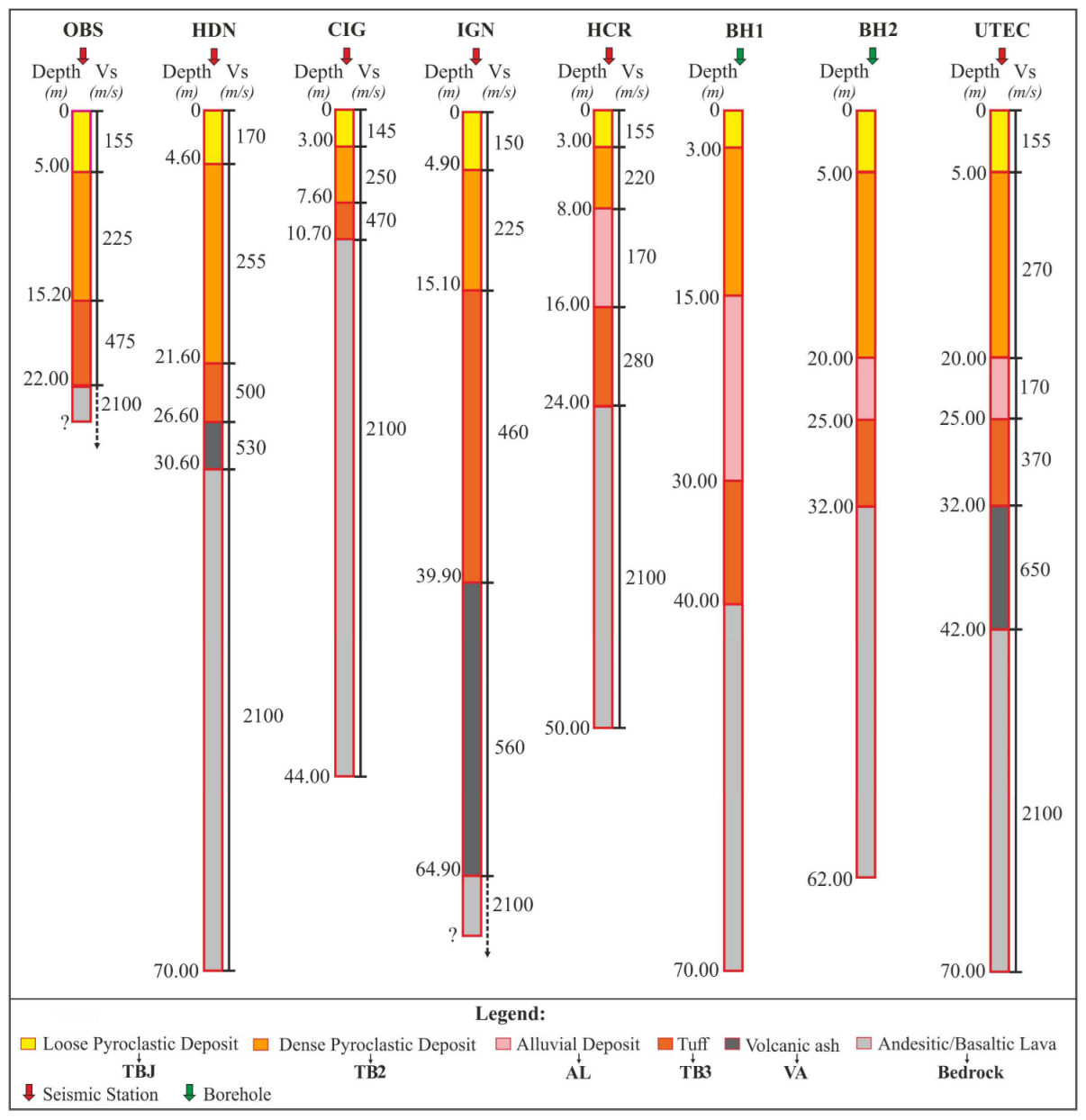
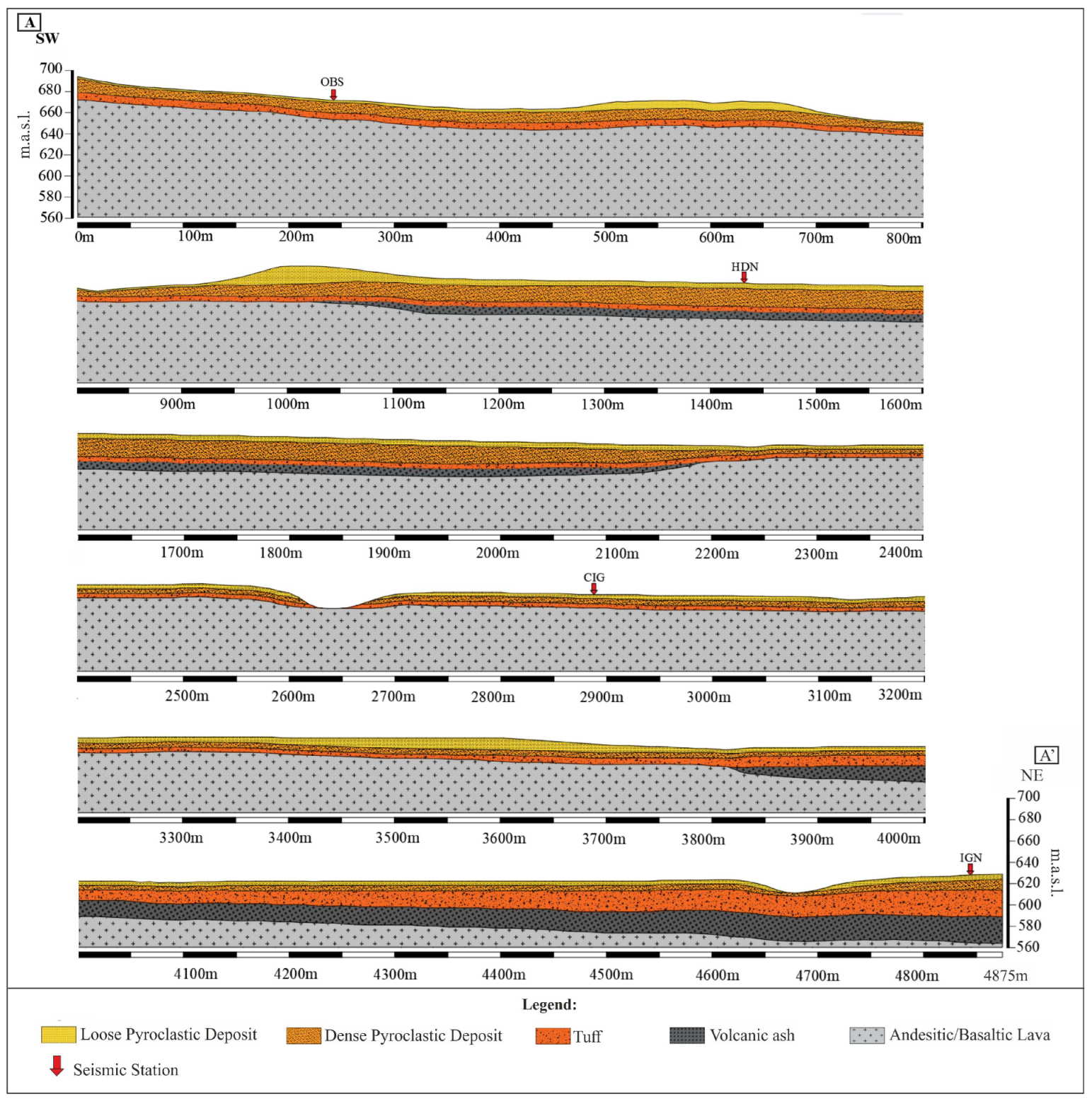
5.2. 2D Subsoil Reconstruction

Two sections (Figure 3) were considered to reconstruct and simulate the two-dimensional dynamic behaviour of the subsoil beneath MASS territory. These sections were characterized by Down Hole tests (DH), Ambient Seismic Noise Measurements (HVSR), Seismic Refraction test (SR), and Boreholes (BH) [25,28,62,63,64].
Table 4 shows the type and number of the geophysical and geo-lithological investigations of the above sites.
An important process of homogenization of the available data has been carried out to uniquely characterize, in terms of thickness, lithotype, and VS the different geological units recognized at the eight stations investigated. Figure 4 shows the simplified litho-technical profiles reconstructed under the eight investigated sites.
In Figure 4, the following soil units can be distinguished from the top to the bottom: (1) The Tierra Blanca Joven (TBJ) consisting of a loose pyroclastic deposit layer of varying thickness; (2) the dense pyroclastic deposit (TB2) with a maximum thickness of 17 m at HDN station; (3) the alluvial deposit (AL) that is detected in BH1 and BH2 boreholes and at HCR and UTEC stations where it causes the velocity inversion; (4) the tuff unit (TB3) which reaches the maximum thickness of 25 m at IGN station, (5) the volcanic ash (VA) that is detected on at HDN, IGN and UTEC stations, whose maximum thickness is 25 m (at IGN station), and (6) the Andesitic and Basaltic lava formation that constitute the geological and seismic bedrock at different depths: the shallowest is reached at CIG station at 10.70 m while the deepest at IGN station at 64.90 m depth. Concerning the water table level, it is at about 30 m under the walking level, although it varies within the municipality territory [56,65].
The two reconstructed subsoil sections are shown in Figure 5 and Figure 6. They are orthogonal to each other (Figure 3) and these two 2D results can be used in a Microzonation map where the surface linear data shall be extended to the urban area.
The first section (AA′) is traced along the SW-NE direction for a total length of 4875 m. It shows, starting from the surface, the following units: TBJ, TB2, TB3 and VA. All the above units rest on a bedrock consisting of basaltic/andesitic lavas (Bedrock).
The thickness of the deposits is not constant along the section but shows evident lateral variations. In particular, the TBJ and the TB2 have a maximum thickness of 17 m that tends to decrease towards the NE until about 4 m. The tuff is present along the whole section and has an almost constant thickness of about 8 m for the first 3.5 km, and then increases towards the NE until it reaches 25 m. The volcanic ash, assumed as lenticular deposits with pinch-out structure, are absent in the OBS and CIG sites, while they are present in the central portion of the model with thicknesses of about 8 m and, in the extreme NE portion, show thicknesses up to 25 m.
The bedrock is located about 100 m below the ground floor. The topography is almost flat and shows isolated shallow depressions (<10–20 m). The layers have few variable gradients and lay, in almost all points, sub-horizontally.
The second section (BB′), which measures 3976 m in length, is oriented perpendicular to AA′ in the NW-SE direction. It consists, from the surface, of the following units: TBJ, TB2, TB3, and ASS resting on a bedrock consisting of basaltic/andesitic lavas. The pyroclastic deposits are intercalated with the alluvial deposits (AL) because they were covered by the pyroclastic deposits during the last explosion of the Ilopango caldera. These alluvial deposits intercepted by the two surveys (BH1 and BH2) and confirmed by the inversion of the Vs values present in the DH of the seismic station HR, are represented within the section as a single lenticular body of varying thickness, whose maximum value is 17 m in the northern part of the model for about 600 m and then decreasing progressively towards the SE.
As for the thickness of the TBJ, it is almost constant along the section while the medium compact pyroclastic deposits are extremely variable: in fact, their thickness varies from a few meters up to 17 m.
The bedrock is located about 100 m below the ground level and outcrops for 155 m at a distance of 3350 m. The topography shows slight shallow isolated depressions that enlarge where the lava outcrops. The layers show mild slopes and, in almost all points, lay sub-horizontally.

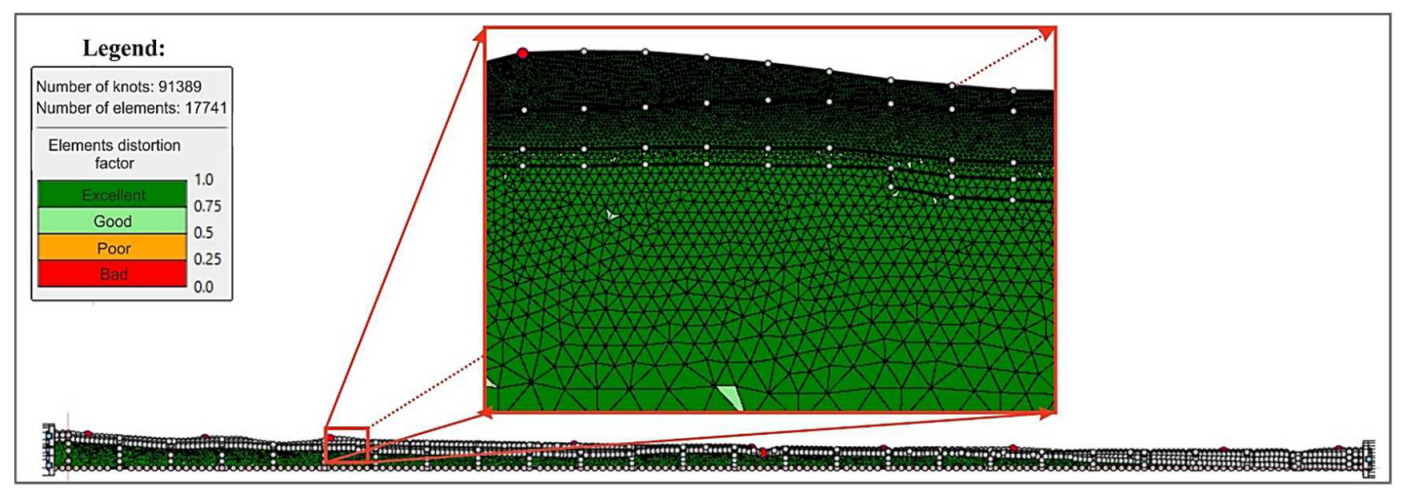
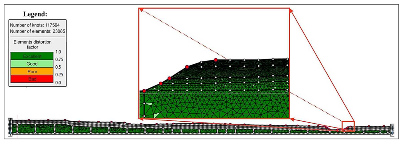
5.3. 2D numerical Models

Both the litho-technical sections AA′ and BB′ (Figure 5 and Figure 6) have been transformed into 2D numerical models to be implemented in LSR2D code [19] (Figure 7 and Figure 8).
The dynamic Poisson coefficient ν was determined by the following relationship:
ν = 1 2 · V p V s 2 1 V p V s 2 1
Table 5 shows the mechanical properties used in both numerical models.
The Figure 9a,b show the G/G0 and D EPRI(93) [66] curves used for the 2D numerical analyses.
The numerical models were discretized in meshes of 17,741 and 91,389 triangular elements for AA′ (Figure 7) and 117,594 and 23,085 triangular elements for BB′ (Figure 8) sections, respectively. The element size was defined according to the rule in Equation (3). The boundary conditions at the vertical boundaries are the wave damping conditions that simulate the semi-infinite domain. Finally, the input motion has been applied to the bottom of both 2D models.

5.4. Input Motions for 2D Numerical Simulation

The input motion used in 2D numerical analyses consists of four accelerograms (the two horizontal components EW and NS, shown in Figure 10) recorded at the Panchimalco (UCA-PA) (see the green triangle in the inset in Figure 1) seismic station of the two mainshocks that occurred on 13 January and 13 February 2001.
These accelerograms are available from the COSMOS Virtual Data Center database [67] by USGS. These waveforms were recorded at a rocky site at the 0.05 s time step. This input selection is due to the scenario-based simulations of the strong and harmful 2001 seismic events. In any case, the authors are aware of the influence of the input motion selection on the seismic response results [68].
The authors used a compliant base where the input upward motion was applied. The upward motion was not the recorded ground shaking (Figure 10). This latter is called the “outcropping motion”, hence it must be propagated downward through a bedrock column at the model bottom (Figure 7 and Figure 8). This input motion is called “incoming signal”. This operation is called “input motion deconvolution” and the authors used the code STRATA [69] to perform it.
Table 6 shows the peak ground accelerations of the four signals used as input motions in the numerical simulations.

6. Results

The results from 2D numerical simulations have been shown through the Amplification Factors (FA), Acceleration Spectra (SA) and Amplification Functions at meaningful locations along the two-section models. The FA have been calculated in three different period ranges, which are 0.1–0.5 s, 0.4–0.8 s and 0.7–1.1 s (Equation (4)). These period ranges have been considered to evaluate the amplification effects at low, medium, and long periods. These three period ranges can differently influence structures of different slenderness [61].
Ten Locations have been selected, five for each section, to show how much the local seismic response changes along the considered sections whose topographic profiles are almost planar and regular, but their underground geometries laterally vary and generate unexpected local amplifications. For this reason, even the Amplification Functions have been calculated, as the ratio, period by period, of the output and the input SA functions.

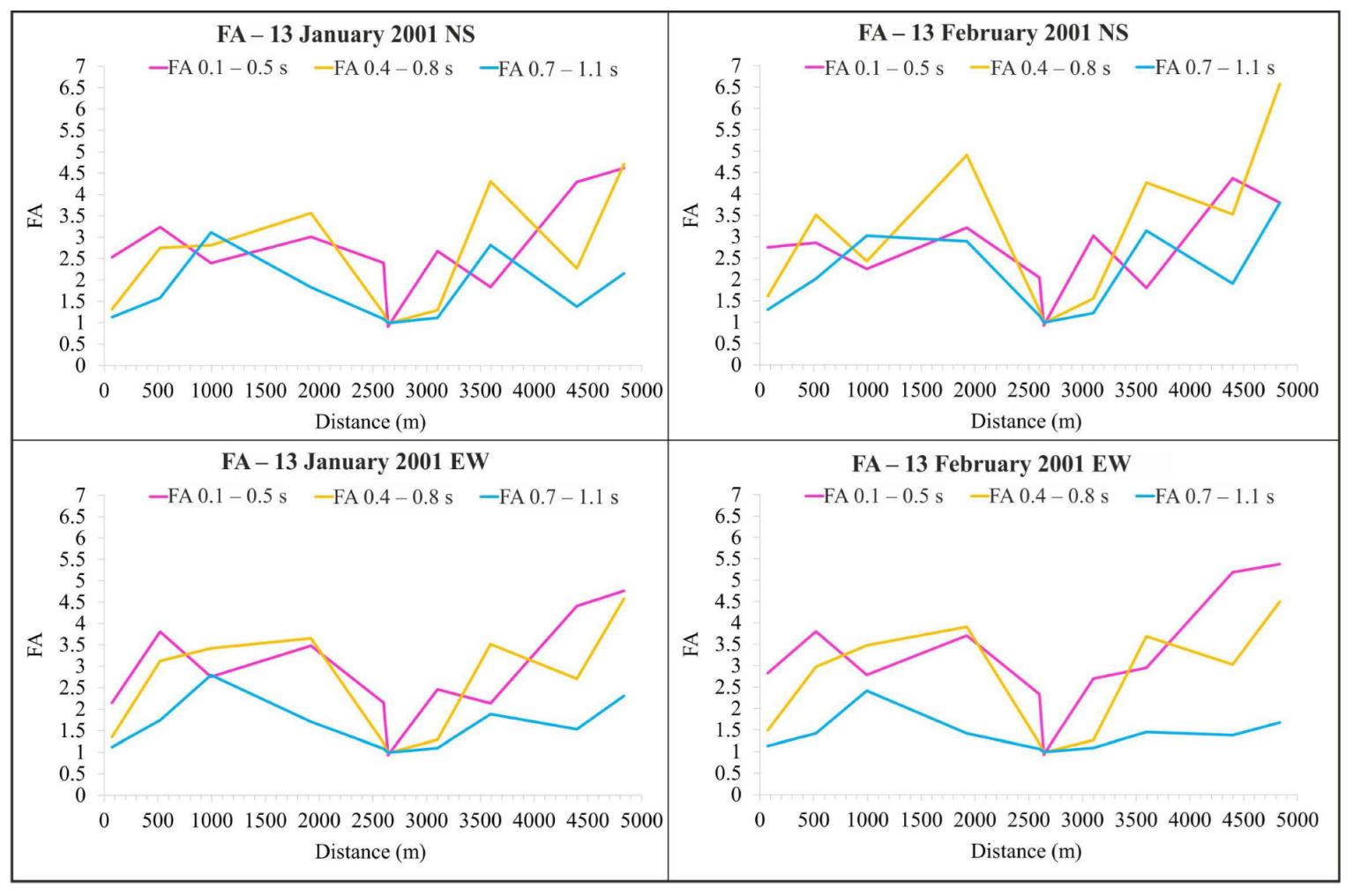
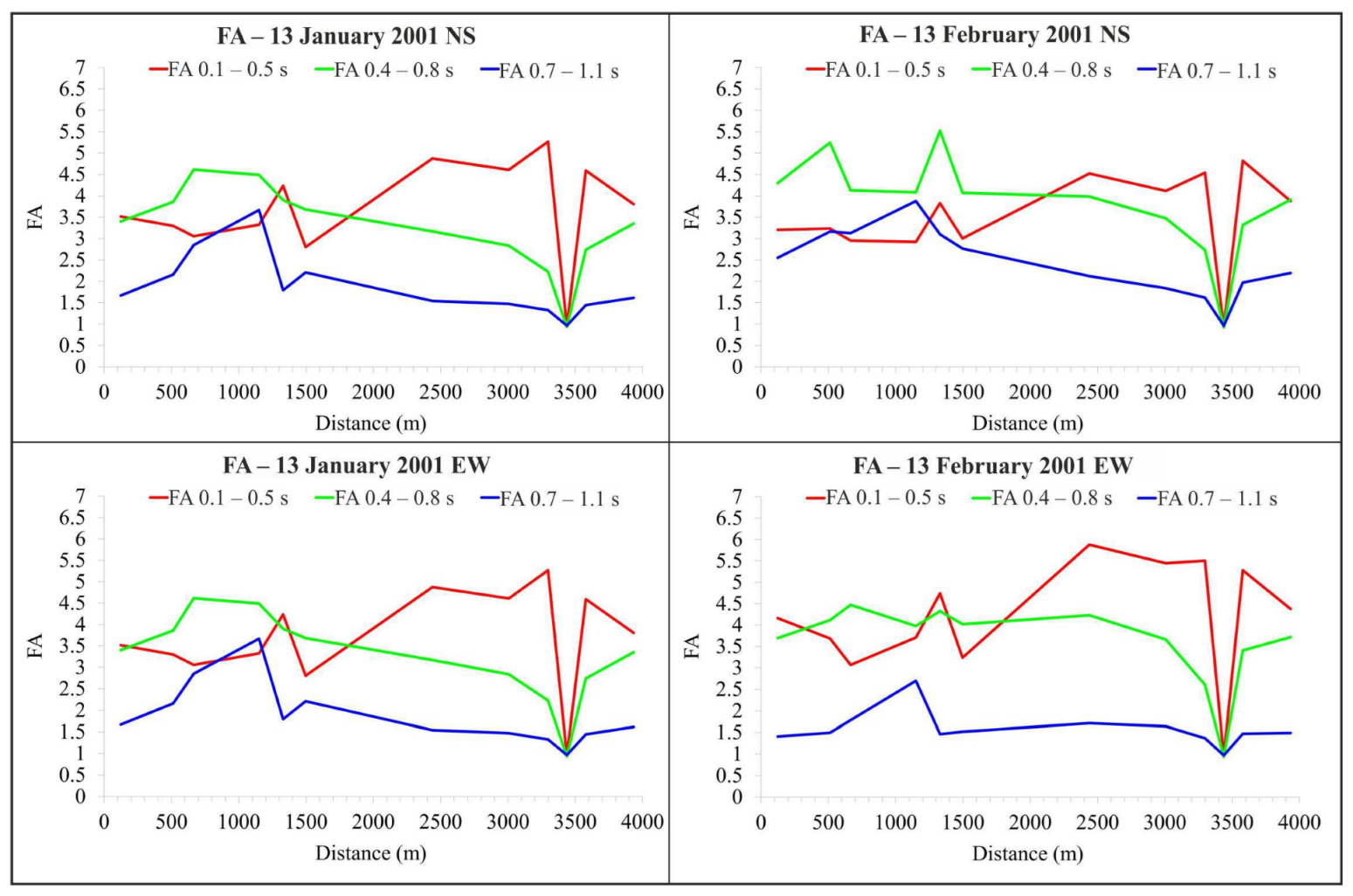
6.1. Amplification Factors

In Figure 11 and Figure 12, the FAs in the three period ranges (0.1–0.5 s, 0.4–0.8 s, 0.7–1.1 s) are reported alongside the two sections (AA′ Figure 5 and BB′ Figure 6) and for each input motion (13 January and 13 February 2001) and each accelerogram component (NS and EW), as reported in the title of each window. The results discussed for the ten locations do not constitute all the results calculated. For this reason, the FA continuous lines are interpolated over 40 points. As can be noted from Figure 11 and Figure 12, the rapid decrease to 1 at 2640 m (section AA′) and 3500 m (section BB′) of all FA values is due to the outcropping seismic bedrock; that is, the lava formation.
The FA values vary along both sections: in section AA′, they range from 1 to 6.5; in section BB′ they vary from 1 to 6. FA values increase towards the Northeast along section AA′ while they show an irregular pattern along section BB′. The highest FA values are related to the period ranges 0.1–0.5 s and 0.4–0.8 s along both sections. These results show a higher vulnerability of buildings with up to eight floors in this area of San Salvador Municipality.
The FA peak values along AA′ section for the four input motions can be recognized at 500, 1900, 2600, 3600 and 4800 m. The FA peaks along the BB′ section are found at 500, 1400, 2500 and 3300 m. At these points, for section AA′ and BB′, the SA functions will be discussed in Section 6.2.
The very high FA value of 6.5 at 4835 m along section AA′ (Figure 11, top window on the right) can be reasonably attributed to the increased thickness of the tuff and volcanic ash layers. There they reach 48 m in thickness (Figure 5). Nonetheless, this high FA value is reached only for the NS component of the 13 February mainshock. Although the local subsoil conditions are responsible for the increase in FA values on the surface, the input motion interferes with them, possibly contributing to increasing these amplifications.

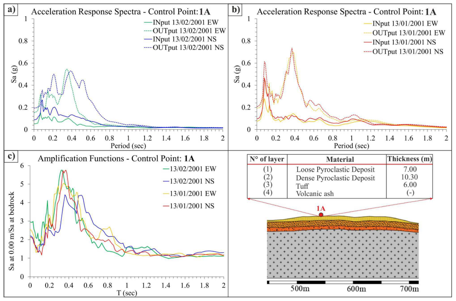
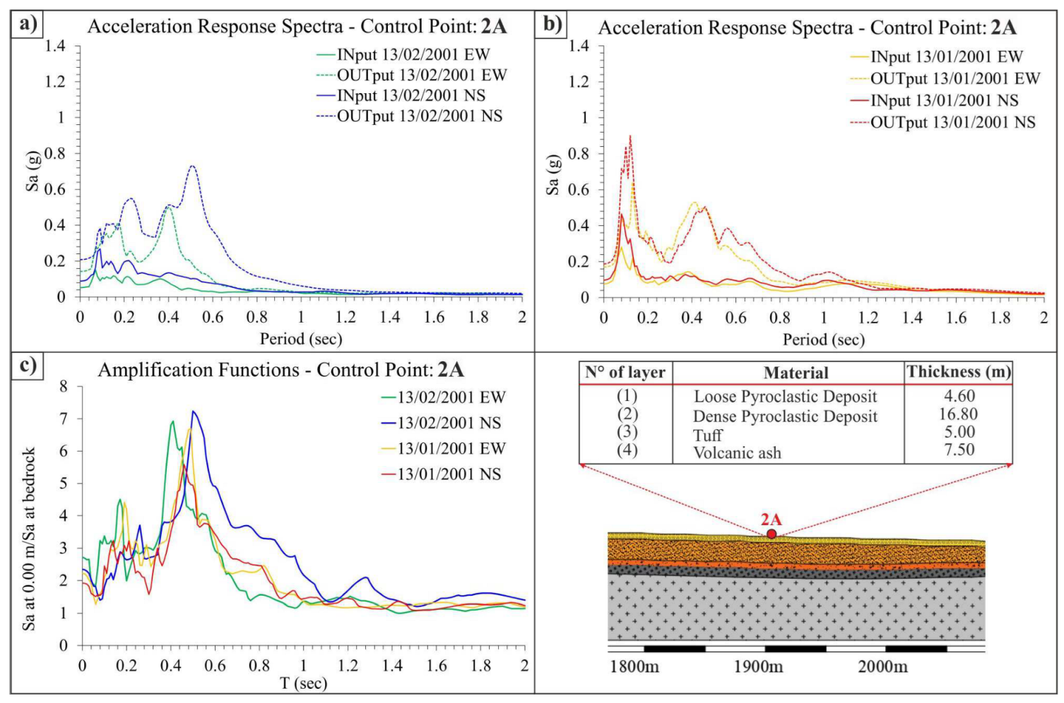
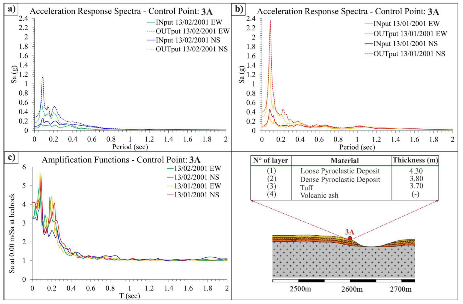
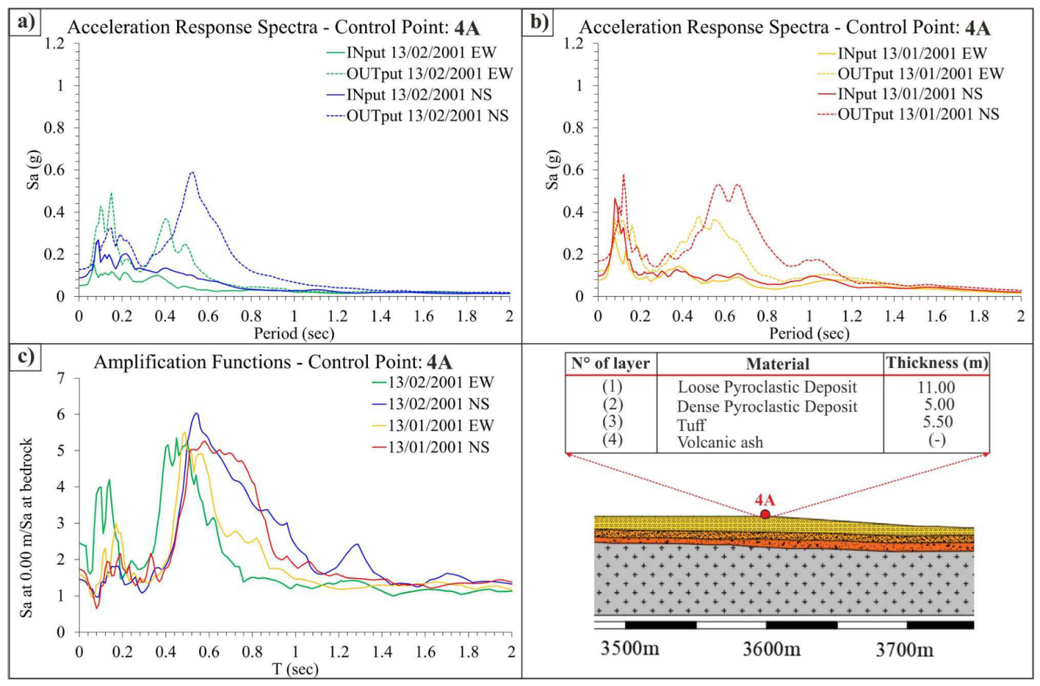
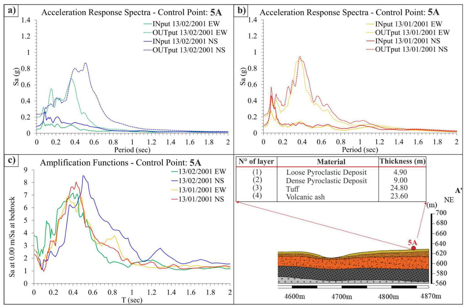
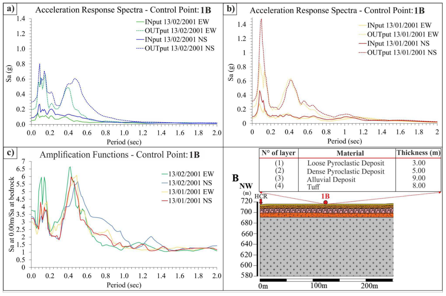
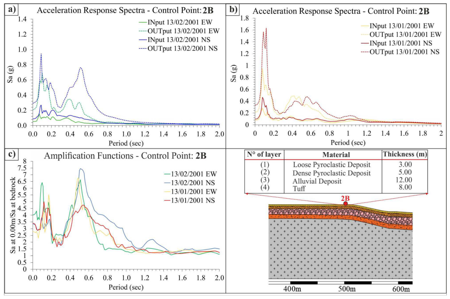
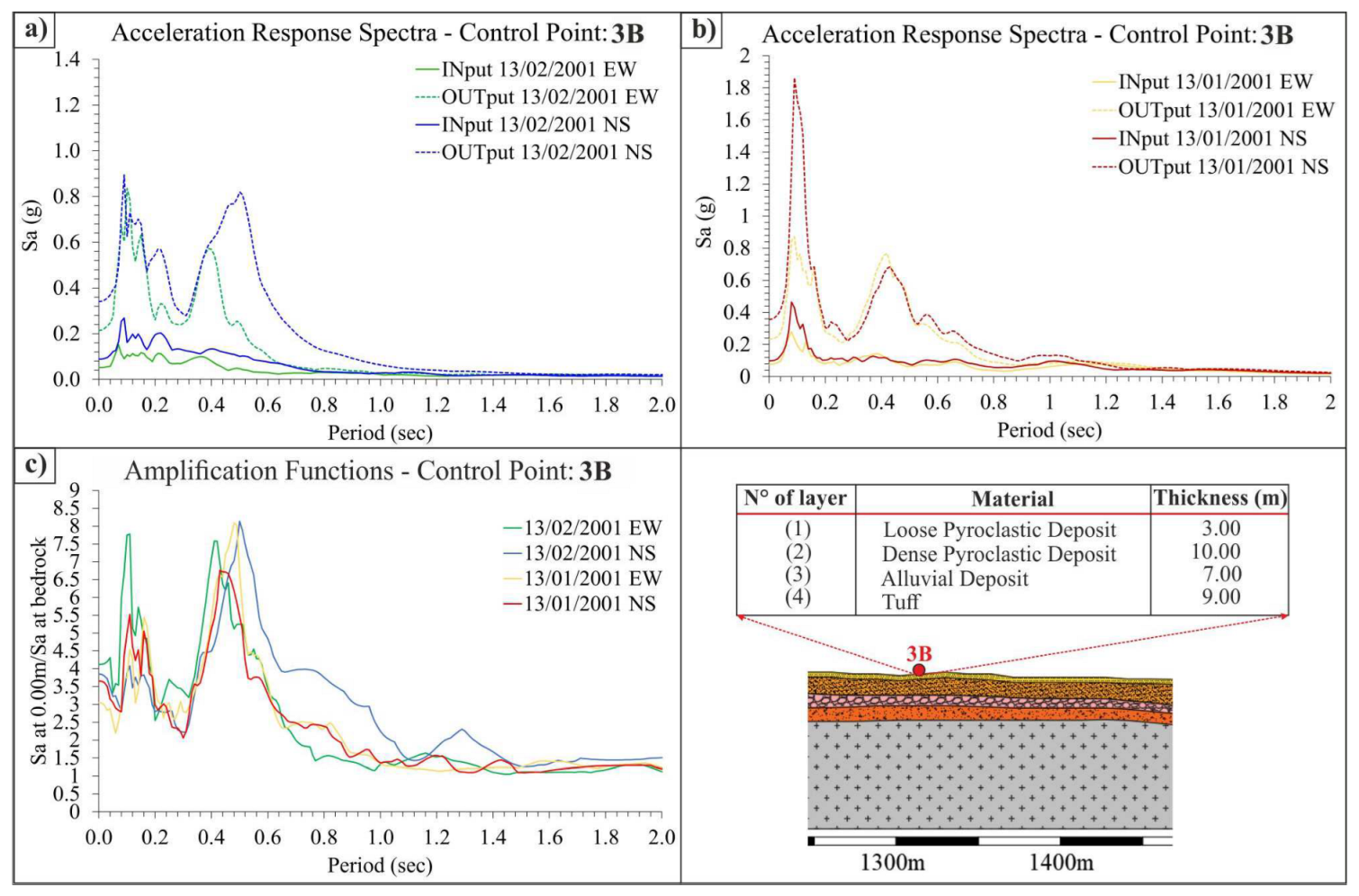
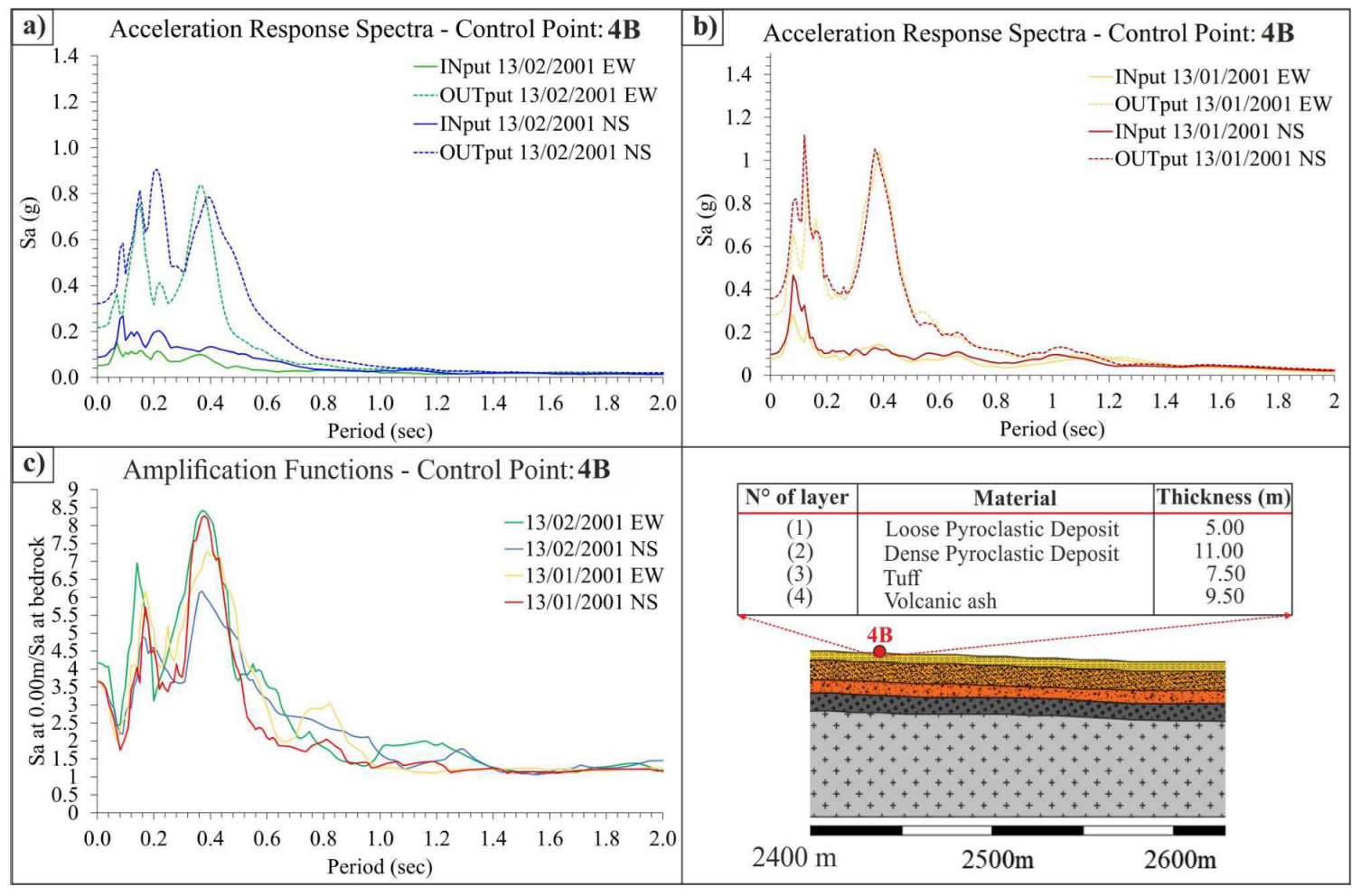
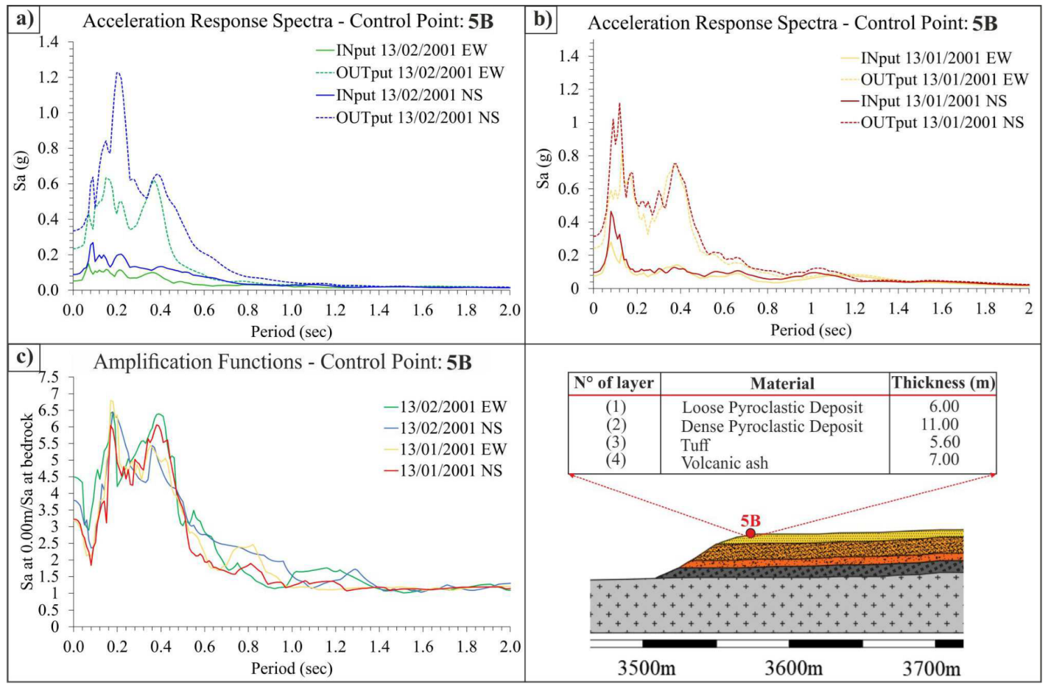
6.2. Acceleration Response Spectra and Amplification Functions

Comparisons of the input and the output SA functions at the numerical control points on the surface of section AA′ are shown in Figure 13, Figure 14, Figure 15, Figure 16 and Figure 17, for the two components (EW and NS) of the two strong motions on 13 January and 13 February 2001. In Figure 13a,b, the seismic response shows two significant peaks: one at low periods (at about 0.15 s) and one at higher periods (at about 0.4 s). The peak at the low period follows the input peak and could be induced by the tuff formation. The peak at 0.4 s is due to the complete soil succession made up of loose and dense pyroclastic deposits. This evidence is also pointed out in the amplification function, Figure 13c, which shows a high peak of 6 at 0.4 s for three out of four input motions. Up to 0.9 s the amplification functions show values varying from 2 to 4.
At numerical control point 2A (Figure 14), again the amplifications are generated not only at the period of the input motion peak (0.15 s) but at longer ones. It can be seen that, due to the larger thickness of the deposits overlaying the bedrock, the amplifications are shifted to 0.45–0.55 s periods. In Figure 14a, for NS component of the February event there are peaks at 0.2 s, 0.4 s and 0.5 s: the highest is the one at 0.5 s equal to 0.73 g. These peaks are confirmed by the January event (Figure 14b) although the highest is set at 0.12 s (0.9 g) and the others, from 0.4 s to 0.65 s, are lower (ranging from 0.35 to 0.5 g).
Amplification functions (Figure 14c) show peaks in the period range 0.4 s–0.5 s of 7, although up to 1.0 s, the amplification functions show values from 3.5 to 2. The high value of the amplification is due to the thickness of the deposits that is larger than 30 m.
At numerical control point 3A (Figure 15), that is located at a distance of about 2600 m from the beginning of the section, the FA value is lower than the one at the previous locations (due to the thinner deposits layers) although the peak FA can be calculated in the period range 0.1–0.5 s. In Figure 15a,b, it can be seen that for all the input motions, the site amplifies the input peak, that is about 0.12 s, although the input motions from the 13 January mainshocks induced a SA peak of 2.4 g. Accordingly, the amplification functions (Figure 15) show two peaks: at 0.08 s, that is 2.8, and at 0.2 s, that is 2. At higher periods, the site de-amplifies the input motion. This is confirmed by the SA, whose output ordinates are lower than the input SA ones. This behaviour is due to the small thickness of the deposits, especially the TBJ, and to the local surface shape: it is a slope that borders a fluvial riverbed.
At the numerical control point 4A (Figure 16), placed about 3600 m from the beginning of the section, there are multiple peaks at low and high period ranges: at about 0.12 s, there is the output SA peak related to the input motion, then in the ranges 0.4–0.55 s (for the February motions) and 0.5 s–0.7 s (for the January motions) the SA peaks reach about 0.6 g.
It can be noted that the overall thickness of the most superficial layers (TBJ and TB) with an average shear wave velocity (Vs) of 200 m/s is 16 m: this thickness could cause the amplification to be kept high and to move towards longer periods (range 0.5 s–0.7 s), thus attenuating the peaks of the amplification functions. These functions (Figure 16c) show two peaks: one at 0.12 s, that is 4 at most, and one ranging from 0.4 to 0.8 s, which varies from 5 to 6.
The tuffs, however, despite having higher seismic velocity but very low thickness (3.80 m), do not contribute to amplifying the motion on the surface but continue to be responsible for the peak at low periods as the input motions (0.12 s).
Figure 17 shows the spectral response of the numerical control point 5A at a distance of about 4835 m from the beginning of the model.
At this point the thicknesses of the deeper deposits such as tuff and volcanic ash become gradually greater assuming a total thickness of 48 m and decrease the thickness of the shallower deposits (12 m). This stratigraphic arrangement shows almost similar responses (in terms of spectral acceleration) for both strong motions amplifying a range of periods varying from 0.4 s to 0.5 s of about 1 g.
A small amplification at 0.12 s is also evident, according to the input motion.
The amplification functions, in Figure 17c, show amplifications ranging from 6 to 8 in the period range 0.3–0.6 s. This 62 m thickness of the deposits overlaying the bedrock explains the large amplification at higher periods.
Similar results can be observed along section BB′: the five numerical control points analysed in Figure 18, Figure 19, Figure 20, Figure 21 and Figure 22, show the amplification of SA shifted to longer periods than the input motions: at 0.12 s and between 0.4–0.5 s, with the amplification functions that show two peaks correspondingly, varying from 6 to 8 according to the increase in the deposits’ thickness. The presence of the alluvial deposits that show Vs lower than the dense pyroclastic deposits seem not to influence the amplification functions peaks but contribute to move the amplified periods to longer values [70]. Nonetheless, the effects of Vs inversion on the response seismic effects, should be assessed in the litho-technical context and cannot be generalized.
At the numerical control points 4B and 5B the alluvial deposits disappear. As a consequence, the amplified periods do not exceed 0.4 s. The amplification function peaks vary from 6 to 8 according to the thickness of the deposits.

7. Discussion on 1D versus 2D Analyses

The analysis of results drawn from the 2D local seismic response simulations in such a geological context could be considered useless because 1D simulations could be sufficient. Hence, we focused on the contribution to shifting the amplified periods of volcanic deposits: the shallow deposits of TB (loose and dense pyroclastic deposits) and the deeper units (tuff and volcanic ash). We considered a 1D approach.
To discriminate the contributions of the aforementioned two groups of volcanic soils, we defined three “cumulated thicknesses”: the first related to the two TB deposits (Ct1), the second related to Tuff and Volcanic ash deposits (Ct2) and the third related to the total thickness of soil deposits overlaying the bedrock (Ct).
Considering the previous numerical control points along the two sections AA′ and BB′ (1A–5A and 1B–5B), we calculated the weighted velocity values of VS of both Ct1, Ct2, and Ct, as follows:
V s w = i = 1 n h i · V s i i = 1 n h i
Along section BB′, the alluvial deposits have been added to the shallower units of TB.
Then, Table 7 and Table 8 compare the 2D amplified periods with the calculated 1D period values based on the three soil groups previously considered, according to the formula:
T 1 D = 4 · H V s w
where the period T1D is referred to 1D behaviour and H can be Ct1, Ct2 or Ct. Table 7, hence, shows that the 1D amplified periods of Ct1 coincides almost at all locations in section AA′ with the amplified period related to the entire soil deposits over the bedrock, Ct. This is not true only in the case of numerical control point 5A, which shows the highest thickness among the five numerical control points. As can be noted from the last column of Table 7, where the amplified periods calculated through the 2D analyses are listed, the two contributions of both Ct1 and Ct2 are recognised by the two amplified ranges of periods. Hence, 1D analyses, should be able to predict only the longer amplified periods, meaning that 1D simulations will be affected by the softer deposits of TB disregarding the role of the Volcanic ash and tuff, that shows the same prevalent period of the considered input motion. Similar results can be drawn along section BB′. Thus, even though the topography of the two sections AA′ and BB′ is almost planar, the lateral variations of the thickness of all the subsoil deposits up to the lava bedrock shows that 1D analyses cannot efficiently predict the amplified periods as 2D simulations do.
These results enable to confirm that buildings of large different heights (from 1 to 7 floors) could have been affected by both strong 2001 earthquakes. According to the simplified equation by NEHRP (94) [71]:
T [ s ] = 0.1 · N
where N is the number of floors and T is the fundamental period of vibration.

8. Conclusions

The RSL has been carried out in the Southeastern portion of the MASS territory along two 2D sections. This territory has been heavily damaged by the two strong earthquakes of 2001and this RSL study shed light on the FA values suffered by this area: from 3.5 to 6.5 along the BB′ section and from 2 to 6.5 along the AA′ section felt in two ranges of periods: 0.1–0.5 s and 0.4–0.8 s.
Such high amplifications in these two ranges of periods are associated with the increase in thickness of the soft TB deposits (at longer periods) but also with the stiffer Tuff and Volcanic ash (at shorter periods). The 2D numerical simulations showed the contribution to the FA values of the variation of the thickness of the deposits along both sections.
These results will be useful to draw the microzonation maps in San Salvador municipality that should be used within the urban planning action to improve the resilience of this territory to the seismic hazard.

Author Contributions

Conceptualization, C.F., G.V., M.L.R.; Methodology, C.F., G.V.; Software, C.F.; Validation, C.F., G.V.; Formal Analysis, C.F.; Investigation, L.A.C.R., M.L.R., J.A.C.; Resources, S.C., M.L.R., J.A.C., L.A.C.R.; Data Curation, S.C., M.L.R., L.A.C.R.; Writing—Original Draft Preparation, C.F., G.V.; Writing—Review & Editing, C.F., G.V.; Visualization, C.F.; Supervision, G.V.; Project Administration, M.L.R.; Funding Acquisition, M.L.R. All authors have read and agreed to the published version of the manuscript.

Funding

This research was funded by the Italian Agency for Development Cooperation (AICS)—CASTES Project—“Establecer y desarrollar la carrera de Licenciatura en Ciencias de la Tierra con énfasis en Geología en la Universidad de El Salvador”.

Data Availability Statement

Data sharing is not applicable to this article.

Acknowledgments

We thank the Italian Cooperation AICS and the CASTES Project. Special thanks to the Researchers of MARN (Ministerio de Medio Ambiente y Recursos Naturales), in the person of the Director Luis Menjivar and Luis Mixco (Responsable of the Monitoring Technician of Multihazards), for their support in data collection activities.

Conflicts of Interest

The authors declare no conflict of interest.

References

  1. Faraone, C.; Colantonio, F.; Vessia, G. Maps of Seismic Amplification Induced by Shallow Cavities Located in Typical Soil Succession of Italian Periadriatic Basin. SSRN Electron. J. 2022. [Google Scholar] [CrossRef]
  2. Stanko, D.; Markušić, S.; Gazdek, M.; Sanković, V.; Slukan, I.; Ivančić, I. Assessment of the Seismic Site Amplification in the City of Ivanec (NW Part of Croatia) Using the Microtremor HVSR Method and Equivalent-Linear Site Response Analysis. Geosciences 2019, 9, 312. [Google Scholar] [CrossRef]
  3. Khanbabazadeh, H.; Iyisan, R.; Ansal, A.; Hasal, M. 2D non-linear seismic response of the Dinar basin, Turkey. Soil Dyn. Earthq. Eng. 2016, 89, 5–11. [Google Scholar] [CrossRef]
  4. Vessia, G.; Russo, S. Relevant features of the valley seismic response: The case study of Tuscan Northern Apennine sector. Bull. Earthq. Eng. 2013, 11, 1633–1660. [Google Scholar] [CrossRef]
  5. Soltani, N.; Bagheripour, M.H. Seismic response analysis of soil profile: Comparison of 1D versus 2D models and parametric study. Model. Earth Syst. Environ. 2020, 6, 1017–1026. [Google Scholar] [CrossRef]
  6. Vessia, G.; Russo, S.; Lo Presti, D. A New Proposal for the Evaluation of the Amplification Coefficient Due to Valley Effects in the Simplified Local Seismic Response Analyses. Ital Geotech. J. 2011, 4, 51–77. [Google Scholar]
  7. Evangelista, L.; Landolfi, L.; d’Onofrio, A.; Silvestri, F. The Influence of the 3D Morphology and Cavity Network on the Seismic Response of Castelnuovo Hill to the 2009 Abruzzo Earthquake. Bull. Earthq. Eng. 2016, 14, 3363–3387. [Google Scholar] [CrossRef]
  8. Zhang, Z.; Fleurisson, J.-A.; Pellet, F.L. A Case Study of Site Effects on Seismic Ground Motions at Xishan Park Ridge in Zigong, Sichuan, China. Eng. Geol. 2018, 243, 308–319. [Google Scholar] [CrossRef]
  9. Moczo, P.; Kristek, J.; Bard, P.-Y.; Stripajová, S.; Hollender, F.; Chovanová, Z.; Kristeková, M.; Sicilia, D. Key structural parameters affecting earthquake ground motion in 2D and 3D sedimentary structures. Bull. Earthq. Eng. 2018, 16, 2421–2450. [Google Scholar] [CrossRef]
  10. Chaljub, E.; Maufroy, E.; Moczo, P.; Kristek, J.; Hollender, F.; Bard, P.-Y.; Priolo, E.; Klin, P.; De Martin, F.; Zhang, Z. 3-D Numerical Simulations of Earthquake Ground Motion in Sedimentary Basins: Testing Accuracy through Stringent Models. Geophys. J. Int. 2015, 201, 90–111. [Google Scholar] [CrossRef]
  11. Primofiore, I.; Baron, J.; Klin, P.; Laurenzano, G.; Muraro, C.; Capotorti, F.; Amanti, M.; Vessia, G. 3D numerical modelling for interpreting topographic effects in rocky hills for Seismic Microzonation: The case study of Arquata del Tronto hamlet. Eng. Geol. 2020, 279, 105868. [Google Scholar] [CrossRef]
  12. Chen, Z.; Huang, D.; Wang, G. A regional scale coseismic landslide analysis framework: Integrating physics-based simulation with flexible sliding analysis. Eng. Geol. 2023, 315, 107040. [Google Scholar] [CrossRef]
  13. Smerzini, C.; Vanini, M.; Paolucci, R.; Renault, P.; Traversa, P. Regional physics-based simulation of ground motion within the Rhône Valley, France, during the MW 4.9 2019 Le Teil earthquake. Bull. Earthq. Eng. 2023, 21, 1747–1774. [Google Scholar] [CrossRef]
  14. Vessia, G.; Rainone, M.L.; De Santis, A.; D’Elia, G. Lessons from April 6, 2009 L’Aquila Earthquake to Enhance Microzoning Studies in near-Field Urban Areas. Geoenvironmental Disasters 2020, 7, 11. [Google Scholar] [CrossRef]
  15. Fayjaloun, R.; Negulescu, C.; Roullé, A.; Auclair, S.; Gehl, P.; Faravelli, M. Sensitivity of Earthquake Damage Estimation to the Input Data (Soil Characterization Maps and Building Exposure): Case Study in the Luchon Valley, France. Geosciences 2021, 11, 249. [Google Scholar] [CrossRef]
  16. Vessia, G.; Laurenzano, G.; Pagliaroli, A.; Pilz, M. Seismic site response estimation for microzonation studies promoting the resilience of urban centers. Eng. Geol. 2021, 284, 106031. [Google Scholar] [CrossRef]
  17. López, M.; Bommer, J.; Méndez, P. The Seismic Performance of Bahareque Dwellings in El Salvador. In Proceedings of the Thirteenth World Conference on Earthquake Engineering, Vancouver, BC, Canada, 1–6 August 2004. [Google Scholar]
  18. OPAMSS (Oficina de Planificación Del Área Metropolitana de San Salvador)—Geoportal. Available online: https://opamss.org.sv/geoportal/ (accessed on 13 March 2023).
  19. LSR2D software—Local Seismic Responce 2D. 2019. Available online: www.stacec.com. (accessed on 1 January 2022).
  20. Bommer, J.; Salazar, W.; Samayoa, R. Riesgo Sísmico En La Región Metropolitana de San Salvador; PRISMA: San Salvador, El Salvador, 1998. (In Spanish) [Google Scholar]
  21. Kattan, C. Advances in the Study of Site Response in AMSS-MARN; Ministerio de Medio Ambiente y Recursos Naturales Dirección General del Observatorio Ambiental Servicio Geológico Nacional: San Salvador, El Salvador, 2011. (In Spanish) [Google Scholar]
  22. Schmidt-Thomé, M. The Geology in the San Salvador Area (El Salvador, Central America), a Basis for City Development and Planning. Geol. Jb. 1975, 13, 207–228. [Google Scholar]
  23. Martínez, H. Microzonificación Sísmica Del Área Metropolitana de San Salvador. Technol. Cienc. UCA 1979, 2, 111–133. (In Spanish) [Google Scholar]
  24. Linares, R. Microzonificación Sísmica de Área Metropolitana de San Salvador Basada En La Observación de Microtemblores, Espectros de Respuesta y Registros de Sismoscopios. Master’s Thesis, University of Central America José Simeón Cañas, San Salvador, El Salvador, 1985. [Google Scholar]
  25. Consorzio El Salvador. Italtekna-Italconsult Evaluación de Peligro Sísmicos En El Área Del Distrito A3 (San Salvador) y El Distrito 7 (Apopa), PARTE 4: Estudio de La Respuesta Sísmica Local y Elaboración de Mapa de Microzonificación Sísmica; 1988. (In Spanish) [Google Scholar]
  26. Aguilar Colato, R.A. Microzonificación En Base a Criterios Geotécnicos, Estimación de Las Propiedades Dinámicas y Análisis de Respuesta Local de Los Suelos Del Área Metropolitana de San Salvador (AMSS). National University of Engineering and Architecture Faculty of Civil Engineering: Japanese Peruvian Seismic Research and Disaster Mitigation Center: International Conference on Microzoning and Safety of Vital Public Service Systems. 1990. Available online: http://cidbimena.desastres.hn/docum/crid/Abril-Mayo2005/CD1/pdf/spa/doc1862/doc1862.htm (accessed on 15 January 2023). (In Spanish).
  27. Guzmán, V.; Linares Guzmán, R.E.; Morales Huezo, M.R. Microzonificación Geotécnica Del AMSS: Primera Etapa; University of Central America: San Salvador, El Salvador, 1996. (In Spanish) [Google Scholar]
  28. Salazar, W.; Seo, K. Spectral and Amplification Characteristics in San Salvador City (El Salvador) for Upper-Crustal and Subduction Earthquakes. In Proceedings of the 11th Japan Earthquake Engineering Symposium (JAEE); Gakkai: Tokyo, Japan, 2002; Volume 65, pp. 329–334. [Google Scholar]
  29. Fonseca, C.E.G. Estudio de respuesta de capas superficiales de suelo en el Área Metropolitana De San Salvador; Universidad Centroamericana “José Simeón Cañas: San Salavador, El Salvador, 2007. (In Spanish) [Google Scholar]
  30. Burgos, E.; Hernandez, D.; Ayala, R.; Pullinger, C. Informe Del Proyecto: Primera Fase de La Microzonificación Sísmica En Las Principales Ciudades de El Salvador, San Salvador, El Salvador. 2007. Available online: https://www.snet.gob.sv/ver/sismologia/riesgo+sismico/amenaza/antecedentes/ (accessed on 15 February 2023). (In Spanish).
  31. Salazar, W.; Sardina, V.; de Cortina, J. A Hybrid Inversion Technique for the Evaluation of Source, Path, and Site Effects Employing S-Wave Spectra for Subduction and Upper-Crustal Earthquakes in El Salvador. Bull. Seismol. Soc. Am. 2007, 97, 208–221. [Google Scholar] [CrossRef]
  32. OPAMSS. NORSAR Earthquake Risk Reduction in Guatemala, El Salvador, and Nicaragua with Regional Cooperation to Honduras, Costa Rica, and Panama, Task 6: Microzonation in San Salvador, Technical Report of the Project Activities, Norway. 2008; OPAMSS: San Salvador, El Salvador, 2008. [Google Scholar]
  33. Crosta, G.B.; Imposimato, S.; Roddeman, D.; Chiesa, S.; Moia, F. Small Fast-Moving Flow-like Landslides in Volcanic Deposits: The 2001 Las Colinas Landslide (El Salvador). Eng. Geol. 2005, 79, 185–214. [Google Scholar] [CrossRef]
  34. Martínez-Díaz, J.J.; Álvarez-Gómez, J.A.; Staller, A.; Alonso-Henar, J.; Canora, C.; Insúa-Arévalo, J.M.; Tsige, M.; Villamor, P.; Herrero-Barbero, P.; Hernández-Moreno, C.; et al. Active faults of El Salvador. J. S. Am. Earth Sci. 2021, 105, 103038. [Google Scholar] [CrossRef]
  35. Canora, C.; Martinez-Diaz, J.; Villamor, P.; Berryman, K.; Álvarez-Gómez, J.A.; Pullinger, C.; Capote, R. Geological and Seismological Analysis of the 13 February 2001 Mw 6.6 El Salvador Earthquake: Evidence for Surface Rupture and Implications for Seismic Hazard. Bull. Seism. Soc. Am. 2010, 100, 2873–2890. [Google Scholar] [CrossRef]
  36. Legrand, D.; Marroquín, G.; DeMets, C.; Mixco, L.; García, A.; Villalobos, M.; Ferrés, D.; Gutiérrez, E.; Escobar, D.; Torres, R. Active Deformation in the San Salvador Extensional Stepover, El Salvador from an Analysis of the April–May 2017 Earthquake Sequence and GPS Data. J. S. Am. Earth Sci. 2020, 104, 102854. [Google Scholar] [CrossRef]
  37. Alonso-Henar, J.; Álvarez-Gómez, J.A.; Martínez-Díaz, J.J. Constraints for the recent tectonics of the El Salvador Fault Zone, Central America Volcanic Arc, from morphotectonic analysis. Tectonophysics 2014, 623, 1–13. [Google Scholar] [CrossRef]
  38. Hernández, W. Características Geotécnicas y Vulcanológicas de Las Tefras de Tierra Blanca Joven, de Ilopango, El Salvador. Master’s Thesis, Polytechnic University of El Salvador, San Salvador, El Salvador, 2004. (In Spanish). [Google Scholar]
  39. Alonso-Henar, J.; Fernández, C.; Álvarez-Gómez, J.A.; Canora, C.; Staller, A.; Díaz, M.; Hernández, W.; García, V.; Martínez-Díaz, J.J. Active Triclinic Transtension in a Volcanic Arc: A Case of the El Salvador Fault Zone in Central America. Geosciences 2022, 12, 266. [Google Scholar]
  40. Martinez-Diaz, J.; Álvarez-Gómez, J.A.; Benito, B.; Hernández, D. Triggering of destructive earthquakes in El Salvador. Geology 2004, 32, 65. [Google Scholar] [CrossRef]
  41. Canora, C.; Martinez-Diaz, J.; Villamor, P.; Staller, A.; Berryman, K.; Álvarez-Gómez, J.A.; Capote, R.; Diaz, M. Structural evolution of the El Salvador Fault Zone: An evolving fault system within a volcanic arc. J. Iber. Geol. 2014, 40, 471–488. [Google Scholar] [CrossRef]
  42. Alonso-Henar, J.; Benito, M.B.; Staller, A.; Álvarez-Gómez, J.A.; Martínez-Díaz, J.J.; Canora, C. Main crustal seismic sources in El Salvador. Data Brief 2018, 20, 1085–1089. [Google Scholar] [CrossRef]
  43. Alonso-Henar, J.; Benito, B.; Staller, A.; Álvarez-Gómez, J.; Martínez-Díaz, J.; Canora, C. Large-magnitude crustal seismic sources in El Salvador and deterministic hazard scenarios. Eng. Geol. 2018, 243, 70–83. [Google Scholar] [CrossRef]
  44. Salazar, W.; Seo, K. Earthquake Disasters of 13 January and 13 February 2001, El Salvador. Seism. Res. Lett. 2003, 74, 420–439. [Google Scholar] [CrossRef]
  45. Bent, A.L.; Evans, S.G.; Rose, W.I.; Bommer, J.J.; López, D.L.; Carr, M.J.; Major, J.J. The MW 7.6 El Salvador earthquake of 13 January 2001 and implications for seismic hazard in El Salvador. Geol. Soc. Am. 2004, 375, 397–404. [Google Scholar]
  46. Atakan, K.; Real, M.C.; Torres, R.; Rose, W.I.; Bommer, J.J.; López, D.L.; Carr, M.J.; Major, J.J. Local site effects on microtremors, weak and strong ground motion in San Salvador, El Salvador. Geol. Soc. Am. Spec. 2004, 375, 321–338. [Google Scholar]
  47. Bommer, J.; Benito, M.; Ciudad-Real, M.; Lemoine, A.; López-Menjívar, M.; Madariaga, R.; Mankelow, J.; de Hasbun, P.M.; Murphy, W.; Nieto-Lovo, M.; et al. The El Salvador earthquakes of January and February 2001: Context, characteristics and implications for seismic risk. Soil Dyn. Earthq. Eng. 2002, 22, 389–418. [Google Scholar] [CrossRef]
  48. Peruzza, L.; Esposito, E.; Amelia, G.C.R.; Pablo, S.; Bernhard, L.E.T.; Giunta, G. MARCA-GEHN, a Prototype Macroseismic Archive of Four Central America Countries. Boll. Geofis. Teor. Ed Appl. 2021, 62, 3–196. [Google Scholar]
  49. Dirección General de Observatorio de Amenazas y Recursos Naturales Estadística de Registros—Cronología de Sismos Destructivos En El Salvador. Available online: http://www.snet.gob.sv/ver/sismologia/registro/estadisticas/ (accessed on 15 February 2023).
  50. López, M.F.; Bommer, J.; Pinho, R. Seismic hazard assessments, seismic design codes, and earthquake engineering in El Salvador. Geol. Soc. Am. 2004, 375, 301–320. [Google Scholar]
  51. CIG. Mappe Isosiste Preliminari per i Terremoti Del 13 Gennaio e Del 13 Febbraio 2001. Available online: http://www.snet.gob.sv/ (accessed on 15 February 2023).
  52. Chávez, J.A.; Valenta, J.; Schröfel, J.; Hernandez, W.; Šebesta, J. Engineering Geology Mapping in the Southern Part of the Metropolitan Area of San Salvador. Rev. Geol. Am. Cent. 2012, 46, 161–178. [Google Scholar]
  53. Lexa, J.; Šebesta, J.; Hernández, W.; Chavez, J.A.; Vásquez, M.E.; Alfaro, I.A. Geología Del Área Metropolitana de San Salvador (1:50,000), El Salvador. Rev. Geol. Am. Cent. 2022, 66, 1–23. [Google Scholar] [CrossRef]
  54. Bosse, H.R.; Lorenz, W.; Merino, A.; Mihm, A.; Rode, K.; Schmidt-Thomé, M.; Wiesemann, G.; Weber, H.S. Carta Geológica de la República de El Salvador (Centroamérica), 100,000. Maps I to VI.; Herausgegeben von der Bunderstalt fur Geowissenschaften und Rohstoffe: Hannover, Germany, 1976; Volume 1. [Google Scholar]
  55. Bommer, J.J.; Rolo, R.; Mitroulia, A.; Berdousis, P. Geotechnical Properties and Seismic Slope Stability of Volcanic Soils. In Proceedings of the 12th European Conference on Earthquake Engineering, London, UK, 9–13 September 2002; p. 695. [Google Scholar]
  56. Rolo, R.; Bommer, J.J.; Houghton, B.F.; Vallance, J.W.; Berdousis, P.; Mavrommati, C.; Murphy, W. Geologic and Engineering Characterization of Tierra Blanca Pyroclastic Ash Deposits; Special Paper of the Geological Society of America; Geological Society of America: Boulder, CO, USA, 2004. [Google Scholar]
  57. Hernández, E.W. Aspectos Geológicos Que Influyen En Las Aguas Subterráneas y En La Respuesta Sísmica Del Área Metropolitana de San Salvador. In Open File Report; Servicio Nacional de Estudios Territoriales: San Salvador, El Salvador, 2008; pp. 1–19. Available online: https://portafolio.snet.gob.sv/digitalizacion/pdf/spa/doc00080/doc00080.htm (accessed on 15 December 2022).
  58. Chávez, J.A.; Hernández, W.; Kopecky, L. Problemática y Conocimiento Actual de Las Tefras Tierra Blanca Joven En El Área Metropolitana de San Salvador, El Salvador. Rev. Geol. Am. Cent. 2012, 47, 117–132. (In Spanish) [Google Scholar] [CrossRef]
  59. Kramer, S.L. Geotechnical Earthquake Engineering; Pearson Education India: London, UK, 1996. [Google Scholar]
  60. Smith, W.D. The Application of Finite Element Analysis to Body Wave Propagation Problems. Geophys. J. R. Astron. Soc. 1975, 42, 747–768. [Google Scholar] [CrossRef]
  61. SM Working Group Guidelines for Seismic Microzonation, Conference of Regions and Autonomous Provinces of Italy—Civil Protection Department, Rome. 2015; (Original Italian Edition: Gruppo di lavoro MS, Indirizzi e criteri per la microzonazione sismica, Conferenza delle Regioni e delle Province autonome—Dipartimento della protezione civile, Roma, 2008, 3 vol. e Dvd). Available online: https://www.protezionecivile.gov.it/it/pubblicazione/indirizzi-e-criteri-la-microzonazione-sismica (accessed on 15 February 2023).
  62. López, J.M.; Mejía, J.A.; Vega, N. Aplicación Del Método de Refracción Sísmica Para La Determinación de Velocidades de Ondas P; University of Central America of El Salvador: San Salvador, El Salvador, 2008. (In Spanish) [Google Scholar]
  63. Barrera De Calderón, M.L. Caracterización Hidrogeoquimíca e Isotopica de Areas de Recarga En El Acuífero de San Salvador. Master’s Thesis, University of Central America of El Salvador, San Salvador, El Salvador, 2010. (In Spanish). [Google Scholar]
  64. González Renderos, A.N.; Palma, S.N.; Vides Escobar, E.D. Caracterización de La Respuesta Sísmica Del Suelo En Catorce Estaciones Acelerográficas de El Salvador Mediante La Estimación de Períodos de Vibración y Perfiles de Velocidad de Corte a Partir de Mediciones de Microtremores; University of Central America José Simeón Cañas: Antiguo Cuscatlàn, El Salvador, 2020. (In Spanish) [Google Scholar]
  65. Nováková, D.H. A hydrogeological study of the northern parts of the La Libertad, San Salvador, and Cuscatlán Districts in El Salvador: A regional and integrated study. Environ. Geol. 2007, 53, 27–33. [Google Scholar] [CrossRef]
  66. Electric Power Research Institute(EPRI). Guidelines for Determining Design Ground Motions; EPRI: Washington, WA, USA, 1993. [Google Scholar]
  67. COSMOS Virtual Data Center. Available online: https://www.strongmotioncenter.org/vdc (accessed on 15 January 2022).
  68. Guzel, Y.; Elia, G.; Rouainia, M.; Falcone, G. The Influence of Input Motion Scaling Strategies on Nonlinear Ground Response Analyses of Soft Soil Deposits. Geosciences 2023, 13, 17. [Google Scholar] [CrossRef]
  69. Kottke, A.R.; Wang, X.; Rathje, E.M. Technical Manual of STRATA Geotechnical Engineering Center; Department of Civil, Architectural and Environmental Engineering, The University of Texas at Austin: Austin, TX, USA, 2013. [Google Scholar]
  70. Fabozzi, S.; Catalano, S.; Falcone, G.; Naso, G.; Pagliaroli, A.; Peronace, E.; Porchia, A.; Romagnoli, G.; Moscatelli, M. Stochastic approach to study the site response in presence of shear wave velocity inversion: Application to seismic microzonation studies in Italy. Eng. Geol. 2021, 280, 105914. [Google Scholar] [CrossRef]
  71. Building Seismic Safety Council. NEHRP Recommended Provisions for the Development of Seismic Regulations for New Buildings, Part I: Provisions, Developed for the Federal Emergency Management Agency; Building Seismic Safety Council: Washington, DC, USA, 1994. [Google Scholar]
Figure 1. The geographical setting of El Salvador region. The inset shows the faults distribution throughout the country and epicentres of the two strong earthquakes (13 January and 13 February 2001). The red arrow indicates the study area (after [37,38], modified).
Geosciences 13 00116 g001
Figure 2. Areal distribution of the number of storeies within the municipality area of San Salvador. (after, [18], modified).
Geosciences 13 00116 g002
Figure 3. Geological map of the Metropolitan Area of San Salvador city (MASS). SSF—San Salvador Formation, CF—Cuscatlàn Formation, BF—Bálsamo Formation. The inset shows the trace of the 2D geo-lithological sections (after [54] modified).
Geosciences 13 00116 g003
Figure 4. Seismic-litho-technical sections of eight sites located within the MASS area are used for the reconstruction of both subsurface models (AA′, BB′).
Geosciences 13 00116 g004
Figure 5. AA′ section of the subsoil at MASS (see Figure 3).
Geosciences 13 00116 g005
Figure 6. BB′ section of subsoil at MASS (see Figure 3).
Geosciences 13 00116 g006
Figure 7. Mesh pattern, number of knots and elements of the 2D numerical model (AA′ section).
Geosciences 13 00116 g007
Figure 8. Mesh pattern, number of knots and elements of the 2D numerical model (BB′ section).
Geosciences 13 00116 g008
Figure 9. (a) G(γ)/G0 and (b) D(γ) EPRI (93) curves used for both 2D numerical simulations.
Geosciences 13 00116 g009
Figure 10. Time histories and response spectra of four accelerograms used as input motion for 2D numerical simulations.
Geosciences 13 00116 g010
Figure 11. Calculated FA values along the section AA′, related to three period ranges (0.1–05 s, 0.4–0.8 s and 0.7–1.1 s), referring to the two components (NS, EW) of the two mainshocks on 13 January and 13 February 2001.
Geosciences 13 00116 g011
Figure 12. Calculated FA values along the section BB′, related to three period ranges (0.1–05 s, 0.4–0.8 s and 0.7–1.1 s), referring to the two components (NS, EW) of the two mainshocks on 13 January and 13 February 2001.
Geosciences 13 00116 g012
Figure 13. Section AA†: numerical control point 1A spectral responses obtained by 2D numerical analyses using LSR2D software. (a) Comparison among the SA of the two components of the 13 February 2001 earthquake. (b) Comparison among SA of the two components of the 13 January 2001 earthquake. (c) Amplification functions related to the four input motions.
Geosciences 13 00116 g013
Figure 14. Section AA′: numerical control point 2A spectral responses obtained by 2D numerical analyses using LSR2D software. (a) Comparison among the SA of the two components of the 13 February 2001 earthquake. (b) Comparison among SA of the two components of the 13 January 2001 earthquake. (c) Amplification functions related to the four input motions.
Geosciences 13 00116 g014
Figure 15. Section AA′: numerical control point 3A spectral responses obtained by 2D numerical analyses using LSR2D software. (a) Comparison among the SA of the two components of the 13 February 2001 earthquake. (b) Comparison among SA of the two components of the 13 January 2001 earthquake. (c) Amplification functions related to the four input motions.
Geosciences 13 00116 g015
Figure 16. Section AA′: numerical control point 4A spectral responses obtained by 2D numerical analyses using LSR2D software. (a) Comparison among the SA of the two components of the 13 February 2001 earthquake. (b) Comparison among SA of the two components of the 13 January 2001 earthquake. (c) Amplification functions related to the four input motions.
Geosciences 13 00116 g016
Figure 17. Section AA′: numerical control point 5A spectral responses obtained by 2D numerical analyses using LSR2D software. (a) Comparison among the SA of the two components of the 13 February 2001 earthquake. (b) Comparison among SA of the two components of the 13 January 2001 earthquake. (c) Amplification functions related to the four input motions.
Geosciences 13 00116 g017
Figure 18. Section BB′: numerical control point 1B spectral responses obtained by 2D numerical analyses using LSR2D software. (a) Comparison among the SA of the two components of the 13 February 2001 earthquake. (b) Comparison among SA of the two components of the 13 January 2001 earthquake. (c) Amplification functions related to the four input motions.
Geosciences 13 00116 g018
Figure 19. Section BB′: numerical control point 2B spectral responses obtained by 2D numerical analyses using LSR2D software. (a) Comparison among the SA of the two components of the 13 February 2001 earthquake. (b) Comparison among SA of the two components of the 13 January 2001 earthquake. (c) Amplification functions related to the four input motions.
Geosciences 13 00116 g019
Figure 20. Section BB′: numerical control point 3B spectral responses obtained by 2D numerical analyses using LSR2D software. (a) Comparison among the SA of the two components of the 13 February 2001 earthquake. (b) Comparison among SA of the two components of the 13 January 2001 earthquake. (c) Amplification functions related to the four input motions.
Geosciences 13 00116 g020
Figure 21. Section BB′: numerical control point 4B spectral responses obtained by 2D numerical analyses using LSR2D software. (a) Comparison among the SA of the two components of the 13 February 2001 earthquake. (b) Comparison among SA of the two components of the 13 January 2001 earthquake. (c) Amplification functions related to the four input motions.
Geosciences 13 00116 g021
Figure 22. Section BB′: numerical control point 5B spectral responses obtained by 2D numerical analyses using LSR2D software. (a) Comparison among the SA of the two components of the 13 February 2001 earthquake. (b) Comparison among SA of the two components of the 13 January 2001 earthquake. (c) Amplification functions related to the four input motions.
Geosciences 13 00116 g022
Table 1. Seismological parameters for destructive earthquakes in El Salvador region since 1899. A: Volcanic chain; B: Subduction zone. Modified from [44].
No.DateMsDepth (km)Latitude (°N)Longitude (°W)Type of Source
125 March 18995.310 13.65 88.80A
219 July 19125.910 13.87 89.57A
37 September 19157.760 13.90 89.60B
48 June 19176.710 13.82 89.31A
58 June 19175.410 13.77 89.50A
628 April 19195.910 13.69 89.19A
721 May 19327.115012.80 88.00B
820 December 19366.110 13.72 88.93A
925 December 19375.910 13.93 89.78A
106 May 19515.910 13.52 88.40A
116 May 19516.010 13.52 88.40A
127 May 19515.510 13.48 88.45A
133 May 19656.315 13.70 89.17A
1419 June 19827.380 13.30 89.40B
1510 October 19865.410 13.67 89.18A
1613 January 20017.860 13.05 88.66B
1713 February 20016.57 13.62 88.85A
Table 2. The list of the principal strongest earthquakes that have caused damage and casualties in the municipality area of San Salvador [36,46,48,49]. (Mi) is the estimated surface wave magnitude deduced from isoseismal intensity maps.
No.DateMagnitudeDamages
121 March 18396.2 (Mi)Several damages in San Salvador’s capital city
216 April 18546.6 (Mi)The event caused destruction in San Salvador: the capital was relocated to Santa Tecla for a period of five years
38 June 19176.7 (Ms)The event caused destruction in Armenia, Ateos, Quetzaltepeque, and other towns. The earthquake was followed by an eruption of the San Salvador volcano, which resulted in lava flows to the north.
428 April 19195.9 (Ms)Damages at San Salvador
53 May 19655.9 (Ms)The earthquake caused 120 casualties, 400 injured people, and 4000 destroyed dwellings
610 October 19865.4 (Ms)The earthquake caused: 1500 casualties, 10,000 injured, 60,000 destroyed or seriously damaged dwellings and more than 100,000 homeless.
713 January 20017.6 (Mw)The earthquake caused: 944 casualties, 1155 public buildings disrupted, 108,261 destroyed dwellings, 19 damaged hospitals, 405 damaged churches and 445 landslides.
813 February 20016.6 (Mw)The earthquake caused: 315 casualties, 82 public buildings disrupted, 41,302 destroyed dwellings, 5 damaged hospitals, 73 damaged churches, 71 landslides.
94 October 20174.8 (Mw)The seismic event caused VIIMM over MASS territory
Table 3. Damage after the two main shocks of 13 January and 13 February 2001 observed in San Salvador department (after [44]).
San Salvador Department
CasualtiesCollapsed HousesHomeless
13 January 20012410,372107,083
13 February 2001401370
Table 4. Sites investigated for the reconstruction of two-dimensional subsoil models. DH: Down-Hole, SR: Seismic refraction, HVSR: Environmental Seismic Noise Measurements, BH: Borehole (see Figure 4).
Name of the SiteIDType of SiteGeophysic and Geognostic InvestigationReferences
Instituto Geografico NacionalIGNSeismic station2 DH tests, 1 SR test, 1 HVRS measure[25,28,62]
Centro de Investigaciones GeotecnicasCIGSeismic station2 DH tests, 1 SR test[25,28,62]
Hogar del NiñoHDNSeismic station1 DH test, 1 SR test, 1 HVSR measure[25,28,62]
ObservatorioOBSSeismic station1 DH test[28]
Hotel Camino RealHCRSeismic station1 DH test[28]
P1 MetrocentroBH1Borehole1 Borehole test[63]
P3 El SocorroBH2Borehole1 Borehole test[63]
Universidad Tecnológica de El SalvadorUTECSeismic station1 Vs profile [64]
Table 5. Dynamic parameters used in both 2D numerical models for sections AA′, BB′: values in brackets are the values used in Section AA′.
MaterialCodeThickness Range
(m)
ρ
(Kg/m3)
Vs
(m/s)
Vp
(m/s)
Poisson
Coefficient
ν (−)
Shear
Modulus
Reduction
Curve
G/G0
Damping D
Curve
Loose Pyroclastic depositTBJ3–6
(2–17)
11221552900.35EPRI (93)
0–6 m
EPRI (93)
0–6 m
Dense Pyroclastic depositTB25–15
(4–14)
1223225
(250)
5600.40EPRI (93)
6–15 m
EPRI (93)
6–15 m
Alluvial DepositAL2–1718201703100.30EPRI (93)
6–15 m
EPRI (93)
6–15 m
TuffTB35–10
(4–25)
2243370
(475)
8900.32
(0.3)
EPRI (93)
15–36 m
EPRI (93)
15–36 m
Volcanic ashVA5–10
(8–25)
2243560
(530)
10900.35EPRI (93)
15–36 m
EPRI (93)
15–36 m
Andesitic/Basaltic LavaBedrockSemi-infinite2447210032400.14Linear = 1Linear = 0.1%
Table 6. Input accelerograms of 13 January and 13 February 2001 selected by COSMOS Virtual Data Center [67].
Station Name & (Code)Station
Coordinates
(Lat, Long)
Date of the EventEvent Time
UTC (hh:mm:ss)
Epicentral
Distance (km)
MwHorizontal ComponentPGA
(g)
Panchimalco (PA)13.6140°
−89.1790°
13 January 200117:33:32857.6NS0.19
EW0.15
13 February 200114:22:05126.6NS−0.18
EW−0.10
Table 7. Amplified periods calculated at 5 numerical control points along the sections AA′.
Control PointsCt1
(m)
Vsw
(m/s)
Ct2
(m)
Vsw
(m/s)
Ct
(m)
Vsw
(m/s)
1D Period Ct1
(s)
1D Period Ct2
(s)
1D Period Ct
(s)
2D Period
(s)
1A17.32156.047523.32820.30.050.30.05–0.1 and 0.2–0.55
2A21.423412.550833.93350.40.10.40.1–0.3 and 0.4–0.7
3A8.12023.747511.82880.20.030.20.03–0.12 and 0.15–0.26
4A16.01865.547521.52600.30.040.30.04–0.2 and 0.4–1.0
5A13.922048.450262.34390.30.40.570.13–0.7
Table 8. Amplified periods calculated at 5 numerical control points along the sections BB′.
Control PointsCt1
(m)
Vsw
(m/s)
Ct2
(m)
Vsw
(m/s)
Ct
(m)
Vsw
(m/s)
1D Period Ct1
(s)
1D Period Ct2
(s)
1D Period Ct
(s)
2D Period
(s)
1B171848370252430.40.070.30.07–0.1 and 0.4–0.6
2B201828370282350.40.070.40.07–0.1 and 0.4–0.7
3B171909370262520.40.080.30.07–0.2 and 0.35–0.7
4B1620317476333440.30.150.40.1–0.5
5B1720012.647629.63170.40.110.40.1–0.5
Disclaimer/Publisher’s Note: The statements, opinions and data contained in all publications are solely those of the individual author(s) and contributor(s) and not of MDPI and/or the editor(s). MDPI and/or the editor(s) disclaim responsibility for any injury to people or property resulting from any ideas, methods, instructions or products referred to in the content.

