Analytical Relation between b-Value and Electromagnetic Signals in Pre-Macroscopic Failure of Rocks: Insights into the Microdynamics’ Physics Prior to Earthquakes

Abstract

Field measurements in subduction regions have revealed the presence of non-seismic pre-earthquake signals such as electromagnetic or acoustic emission, gas liberation, changes in Earth’s surface temperature, changes at the ionospheric level, or fluid migration. These signals are commonly associated with impending earthquakes, even though they often rely solely on temporal and spatial correlations in impending earthquake zones without a comprehensive understanding of the underlying lithospheric processes. For example, one criticism is the measurement of increasing electromagnetic signals even in the absence of observable macroscopic stress changes, which challenges the conventional understanding that macroscopic stress changes are the primary energy source for non-seismic pre-earthquake signals. To address this gap, rock experiments provide valuable insights. Recent experiments have shown that rocks can become electrified under constant macroscopic stress changes, accompanied by a decrease in the b-value, indicating multiscale cracking. This suggests the existence of small-scale dynamics that generate electromagnetic signals independently of large-scale stress variations. In that sense, multiscale thermodynamics offers a valuable perspective in describing this multiscale phenomenon. That is why the main goal of this work is to demonstrate that the electromagnetic signals before macroscopic failures are not independent of the cracking generation because the origin of both phenomena is the same. In particular, we present analytical equations that explain the physical connection between multiscale cracking, the generation of electromagnetic signals, and its negative correlation with acoustic emission before the macroscopic failure of rocks even when the macroscopic load is constant. In addition, we also show that the thermodynamic fractal dimension, which corresponds to the global parameter that controls the cracking process, is proportional to the b-value when the large-scale crack generation is considerably larger than the small-scale cracks. Thus, the decreases in the b-value and the increases in the electromagnetic signals indicate that rocks irreversibly prepare to release energy macroscopically. These findings could be related to the dynamics at lithospheric scales before earthquakes.

1. Introduction

In recent decades, the intricate nature of fracture processes has been a significant area of interest. This is because it has the potential to facilitate the creation of novel materials with enhanced fracture toughness and damage tolerance, as well as more precise models for predicting fracture behavior [1,2,3]. The understanding of this knowledge can have significant implications in various aspects, including the design and maintenance of engineering structures, as well as our comprehension of natural phenomena, such as earthquakes [4,5], and even aiding in the repair of cracks in living bones [6,7,8]. A method of comprehending natural fracture is by studying how rock samples respond under varying conditions, including stress distributions. When brittle materials are subjected to stress, they change their shape by either shortening or lengthening. As stress increases, the material may begin to collapse internally by creating microcracks that follow a fractal pattern. These microcracks continue to grow until they result in macroscopic failure that is also self-similar [9,10,11,12,13,14,15,16,17,18,19,20]. As microcracks grow, they release energy in the form of acoustic emissions and electromagnetic signals. These signals can be used to understand the internal stress states that occur before macroscopic failures [21,22,23,24]. In particular, acoustic and electromagnetic emissions occur due to the movement of crack surfaces when microcracks propagate through a rock sample. This movement generates transient electrical currents by breaking the bonds, which causes a sudden release of energy in the form of elastic waves that propagate through the rock [18,25,26,27,28,29,30,31]. Despite focusing primarily on rock samples, both experimental and theoretical works have attempted to extrapolate their findings to the lithospheric domain. In particular, some researchers have explored the use of electromagnetic signals as a predictive tool for monitoring impending large earthquakes [32,33,34,35,36,37,38,39,40]. Likewise, numerous studies have attempted to establish connections between seismological parameters, such as friction, stress drop, earthquake magnitude, b-value, and large-scale cracking and stresses, through the application of thermodynamic principles [29,41,42,43]. In particular, despite being a matter of actual research [44], the b-value is consistently negatively correlated to tectonic stresses in the context of the buoyancy of the subducting plates [45]. On the other hand, some researchers have applied statistical methods on a larger scale, such as the Gutenberg–Richter law, to analyze rock samples. In doing so, they have used an equivalent b-value and acoustic emissions [46,47,48]. At the laboratory scale, the negative correlation between the b-value and the emission of electromagnetic signals holds true [49,50,51]. Additionally, it has been observed that the b-value also tends to decrease as the applied stress increases in rock samples, as demonstrated by studies such as Dong et al. [52]. However, recent findings suggest that this decrease in the b-value can also be observed under constant stress conditions [51]. This suggests that rocks exhibit small-scale dynamics, emphasizing the need for multiscale formalisms to understand these dynamics across different scales. For example, the multiscale thermodynamics framework provides a suitable approach for comprehending the energy dissipation at various scales concurrently. In these systems, the energy release gives rise to power-law distributions implying that the overall entropy production of the system is determined solely by the dissipation at both large and small scales [42,43]. Consequently, the multiscale thermodynamic perspective of the cracking process highlights that the dissipation of energy, and the underlying dynamics are driven exclusively by the maximum and minimum crack sizes [42,43]. That is why in order to address the apparent contradiction concerning the b-value changes and electromagnetic emission even under constant load before macroscopic failure, and to establish causal connections between them, this study explores the multiscale thermodynamics formalism of crack generation. To achieve this, Section 2 explores the multiscale nature of cracks and their relationship to acoustic emission and electromagnetic signals through fractal thermodynamics, while Section 3 examines the specific case of the balance between small and large stresses in the system. The discussion and conclusions are presented in Section 4 and Section 5, respectively.

2. Electromagnetic Emission and b-Value Relationship: The Physical Foundation

The process of rock damage in a specimen’s body is a consequence of the deformation resulting from applied mechanical loading [24]. Under stress, the rock sample experiences different types of deformation, including elastic strain, plastic deformation, and ultimately, fracture. These deformations are influenced by the inherent strength and properties of the rock material. During the course of deformation, variations in stress within the rock sample can give rise to the generation of electric currents. This intriguing phenomenon arises from the redistribution of charges within the rock material in response to the applied stress. The movement of charged particles engenders electric currents that can be detected and quantified. Both experimental investigations and theoretical analyses have provided evidence supporting the relationship between the rate of stress change $\dot{\sigma }$ and the magnitude of electrical currents ${\widehat{J}}_e$ for uniaxial load, which can be expressed as [53,54]:

$${\widehat{J}}_e\sim \dot{\sigma }$$

(1)

The equation suggests that cracks can be generated by an applied stress change, which then releases electrical currents. A compressive regime with a small but non-zero stress change is represented schematically in Figure 1, where microcracks generate electromagnetic signals that are measured at the rock’s surface (represented by the blue wavy curve). Equation (1) represents the transport of energy between external load and the net electrical currents generated in cracks of different sizes. In that sense, Venegas-Aravena et al. [42] incorporated the self-similarity into Onsager’s relations, which describe the transport of energy in systems out of equilibrium, in order to understand how energy is transferred and distributed within the system across different scales [42,55,56]. This implied that, as macroscopic external forces ($F$) increase, there is a manifestation of the release of excess energy, resulting in the emergence of power-law distributions such as fractally distributed cracks, as well as the reduction of the fractal dimension [42]. Note that this phenomenon is closely associated with an increase in irreversible material damage [10,42,57]. That is why this process can be represented in terms of the increase in entropy $S$, as given by the following equation [42]:

$$dS\sim {\dot{F}}^2={\dot{\sigma }}^2$$

(2)

Multiscale thermodynamics dictates that the relation between the large-scale components (large cracks) and the small-scale components of the system are interrelated as [42]:

$$dS=r^{\alpha }d{S}_0\Rightarrow S=r^{\alpha }\int d{S}_0=r^{\alpha }{S}_0$$

(3)

where $S$ and $S_0$ are the entropy change of the large- and small-scale section of the system, respectively; $r$ is a geometrical factor; and $\alpha$ a is a factor. Conversely, the amplitude of the acoustic emissions $A$ in the magnitude–frequency relationship is determined by the b-value of rock samples as [47]:

$${\log }_{10}N=a-b\times A$$

(4)

where $N$ is the number of events, and $a$ is a constant. The amplitude of the acoustic emission can also be measured at the surface of the rock, as depicted by the red wavy curve in Figure 1. However, the $b$ factor is not constant and may vary in relation to the evolution of entropy $S$, as expressed by [58]:

$$b=b_M{10}^{-H}$$

(5)

where we have considered that $H=S$, $H$ is the Shannon entropy, and $b_M$ is a constant that states the maximum b-value. By replacing Equation (3) with Equation (5), the b-value is:

$$b=b_M{10}^{-r^{\alpha }{S}_0}$$

(6)

The factor $\alpha$ can be written as $\alpha =D_E-D-1$ where $D_E$ is the Euclidean dimension, and $D$ the thermodynamic multifractal dimension, which can be written as [43]:

$$D=-k_V\ln {\mathsf{\Omega }}_V$$

(7)

where $k_V=1/\log \left(r^{\mu }/r_0\right)$, $r^{\mu }$, and $r_0$ are the large- and small-scale length, ${\mathsf{\Omega }}_V={\omega }_{0}dS/d{S}_0$ and ${\omega }_0=e^{(1-D_E)/k_V}$. Thus, the relation between the b-value and the fractal dimension is obtained by replacing Equation (7) with Equation (6):

$$b=b_M{10}^{{-S_{0}r}^{\left(2-D\right)}}$$

(8)

The relationship between the b-value and the fractal dimension of the system is described by Equation (8), although it is important to note that they are not physically equivalent. As the fractal dimension depends on the multiscale properties of the system, a thorough multiscale analysis is necessary to properly interpret Equation (8). Microcracks are typically of the order of 100 $\mathsf{\mu }$m or less [59], while macroscopic failures have a size comparable to the length of rock samples. Thus, there can be a difference of 3 to 4 orders of magnitude between the smallest and largest cracks, depending on the size of the rock sample, ranging from centimeters to meters. Consequently, the values of $r$ must span at least 3 to 4 orders of magnitude. The relationship between $D$ and the entropy change balance ${\mathsf{\Omega }}_V$ (Equation (3)) for a system embedded in a 3D space is depicted in Figure 2a. It is evident from the figure that larger values of $D$ are associated with smaller values of ${\mathsf{\Omega }}_V$. As the relationship between ${\mathsf{\Omega }}_V$ and $D$ can be expressed as ${\mathsf{\Omega }}_V\sim dS/d{S}_0$, it follows that larger values of $D$ imply the dominance of small-scale entropy generation (indicated by the dark yellow dashed line in Figure 2a). Conversely, larger values of ${\mathsf{\Omega }}_V$ are related to smaller values of $D$ which are dominated by large-scale entropy generation (indicated by the red dashed line in Figure 2a). Nevertheless, for the two extremes regimes, the fractal dimension and the entropy change balance exhibit an almost linear relationship:

$$D\sim -\frac{dS}{d{S}_0}$$

(9)

Figure 2b indicates a linear correlation between $D$ and $b$ for both the large- and small-scale entropy releases, where $S_0=1$ and $b_M=2.5$ (shown by the red and dark yellow dashed lines in Figure 2b). Therefore, Equation (8) can be interpreted as follows for a system that is defined by either large- or small-scale entropy releases:

$$b\sim D$$

(10)

To clarify, Equation (10) applies only when either the generation of large-scale cracks or small-scale cracks is significantly more dominant than the other. Thus, taking into account Equations (1), (2), (9) and (10), we can establish a relationship between the b-value, stress change, and electromagnetic signals as follows:

$$b\sim -{\mathsf{\Omega }}_{\dot{\sigma }}\sim -{\mathsf{\Omega }}_{{\widehat{J}}_e}$$

(11)

where ${\mathsf{\Omega }}_{\dot{\sigma }}={\omega }_{\dot{\sigma }}{\dot{\sigma }}^2/{\dot{\sigma }}_0^2$ and ${\mathsf{\Omega }}_{{\widehat{J}}_e}={\omega }_{\widehat{J_e}}{\widehat{J}}_e^2/{{\widehat{J}}_e^2}_0$; $\dot{\sigma }$ and ${\dot{\sigma }}_0$ represent the macroscopic and microscopic stress changes, respectively; ${\widehat{J}}_e$ and ${\widehat{J}}_{e_0}$ the macroscopic and microscopic electromagnetic signals. respectively; and ${\omega }_{\dot{\sigma }}$ and ${\omega }_{\widehat{J_e}}$ constants. Note that the stress change balance ${\mathsf{\Omega }}_{\dot{\sigma }}$ can be conceptualized in a similar manner to the multiscale entropy production balance $\mathsf{\Omega }$ in Equation (7). It involves considering the distribution and exchange of stress at different scales within a system. Just as entropy production characterizes the rate at which entropy is generated within a system, the stress change balance describes the redistribution and transformation of stress at various scales. For macroscopic variations, Equation (11) leads to:

$$b\sim -{\dot{\sigma }}^2\sim -{\widehat{J}}_e^2$$

(12)

Thus, Equation (12) states that there exists a negative correlation between the b-value and the macroscopic electromagnetic signals that are produced due to the cracking process. In situations where Equation (9) does not exhibit a clear linear trend, Equations (9), (11) and (12) can be expressed in a more generalized manner as:

$$\sim -\ln \frac{dS}{d{S}_0}$$

(13)

$$b\sim -\ln {\mathsf{\Omega }}_{\dot{\sigma }}\sim -\ln {\mathsf{\Omega }}_{{\widehat{J}}_e}$$

(14)

$$b\sim -\ln {\dot{\sigma }}^2\sim -\ln {\widehat{J}}_e^2$$

(15)

Figure 3a illustrates the relationship between the b-value and the macroscopic entropy change through ${\widehat{J}}_e$, represented by the green curve. As indicated by Equation (15) (shown by the red curve in Figure 3a), the green curve indicates a negative correlation between the b-value and the increase in electromagnetic signals. Hence, the negative correlation between the b-value and electromagnetic signals is a result of the multiscale entropy change, as Equation (2) encompasses the derivation of both.

3. The Multiscale Stress Evolution

Equations (12) and (15) demonstrate how the b-value reflects macroscopic changes in stress. However, experiments have shown that despite the macroscopic applied stress being almost constant, there is a large variability in the electromagnetic pulses [51]. A schematic representation of this behavior is shown in Figure 3b. The black curve represents the constant macroscopic applied stress, while the blue and red curves depict the negative evolution between the electromagnetic signals and the b-value, respectively. Equations (9), (11) and (14) reveal that the b-value arises from a trade-off between large- and small-scale changes, suggesting the presence of microscopic dynamics and small-scale stress evolution ${\sigma }_0\left(t\right)$ in the system. By employing the definition of ${\mathsf{\Omega }}_{\dot{\sigma }}$ in Equation (11), it becomes possible to determine the microscopic stress states in the following manner:

$${\sigma }_0\left(t\right)=\int \dot{\sigma }\left(t\right)\sqrt{\frac{{\omega }_{\dot{\sigma }}}{{\mathsf{\Omega }}_{\dot{\sigma }}\left(t\right)}}\mathrm{d}t$$

(16)

The pulse-like temporal evolution of ${\widehat{J}}_e$ represented in Figure 3b can be simply modeled as $\sim {\left|t-t_0\right|}^{-0.5}$ which implies that $b\sim -\ln {\left|t-t_0\right|}^{-1}$. This can be seen in Figure 4a as a blue and red curve, respectively. As ${\widehat{J}}_e$ is proportional to the stress balance ${\mathsf{\Omega }}_{\dot{\sigma }}\left(t\right)$ (Equation (11)), it can be obtained by the relation ${\mathsf{\Omega }}_{\dot{\sigma }}\sim {\widehat{J}}_e^2$. This means that ${\mathsf{\Omega }}_{\dot{\sigma }}\left(t\right)$ for this temporal variation is $\sim {\left|t-t_0\right|}^{-1}$ (black curve in Figure 4b). However, the applied stress remains constant. As a result, the macroscopic stress change, $\dot{\sigma }\left(t\right)$, almost disappears as well as Equation (16). Because of the noise in experiments [51], it is difficult to determine whether there is a considerably small linear increase. Therefore, it can be concluded that the macroscopic stress can be defined as $\sigma \left(t\right)=c_{0}t+c_1$ for $c_0\to 0$. This leads that $\dot{\sigma }\left(t\right)\approx c_0$. In a multiscale analysis, it is important to acknowledge that the small constant, although typically negligible compared to the macroscopic constant $c_1$ under normal conditions, cannot be treated as zero. This is because it represents the amplitude of small-scale stress changes. Thus, even though $c_0$ may be several orders of magnitude smaller than $c_1$, it cannot be considered as zero. The magenta curve in Figure 4b represents the almost negligible macroscopic stress change, where $c_0=0.001$, and the figure is presented in its normalized version. Considering the previous analysis, Equation (16) can be applied. The red curve in Figure 4b highlights the microscopical stress change, which demonstrates that the only way to achieve a high ${\mathsf{\Omega }}_{\dot{\sigma }}$, leading to a low b-value and high ${\widehat{J}}_e$, is to decrease the microscopical stresses in the system. This decrease in small-scale dynamics is illustrated in the schematic representations of Figure 4c,d. In the context of fractal thermodynamics, these small-scale dynamics correspond to the dominant generation of small-scale cracks caused by a heterogeneous medium [42]. Figure 4c illustrates this scenario in terms of differential stresses. The small-scale arrows in black and red represent how the small-scale stresses accommodate and transfer the external macroscopic stresses, which are represented by large red and black arrows in Figure 4c. These differential stresses may generate numerous small-scale cracks, which can be detected as a small amplitude of electromagnetic, acoustic emissions, and large b-value. On the other hand, the evolution of ${\mathsf{\Omega }}_{\dot{\sigma }}$ suggests a transition in the dominant scale. Figure 4d demonstrates when large-scale entropy production dominates, as represented by the large-scale stresses filling the medium and leading to the coalescence or growth of small cracks. This implies that the large-scale dynamics are characterized by large-scale cracks. Such a process generates significant electromagnetic and acoustic emissions, which can be readily detected outside the rock samples and reduces the b-value.

4. Discussion

The investigation of non-seismic electromagnetic signals in relation to large seismic events such as megathrust earthquakes is a highly relevant and challenging field of study. Currently, many researchers studying these signals do not establish clear links between their findings and actual earthquakes, and few of them offer proper explanations for the underlying causal mechanisms [60,61,62,63,64,65,66,67,68,69,70]. As a result, the scientific community focusing on non-seismic pre-earthquake signals is still far from providing reliable tools for earthquake forecasting to seismologists who expect to understand the causal mechanisms associated with ruptured parameters of faults, such as seismic moment rate, rupture velocity, final slip distribution, and the sources of high-frequency ground motion. To advance our understanding of earthquake processes, it is crucial to delve into the dynamics of the lithosphere and the variations that natural faults undergo before an earthquake. The multiscale cracking process is particularly pertinent in this context as it may be influenced by the same dynamics that impact the faults where earthquakes’ ruptures nucleate, evolve, and arrest. In that sense, both the rupture generation and the emergence of cracks before macroscopic failure can be regarded as an irreversible multiscale phenomenon occurring when heterogeneous materials are subjected to increasing external stresses over time [42,71,72]. In this context, the generation, growth, and coalescence of microcracks play a critical role as precursors to macroscopic failure [16,73,74,75]. Moreover, the development and interaction of microcracks within the material are intimately connected to the observed changes in the b-value, amplitude of acoustic emissions, and electromagnetic signals, which serve as valuable indicators of the impending failure of heterogeneous materials. For example, the amplitude of acoustic and electromagnetic signals increases as the material approaches failure, as observed in previous studies [49,50,76]. Conversely, the b-value tends to decrease [51]. The connection between the b-value and acoustic emission is not yet fully understood. It is recognized that small cracks within materials, associated with small-scale dynamics, generate low-amplitude acoustic emissions, resulting in large b-values. On the other hand, large-scale cracks lead to a decrease in the b-value, and this reduction becomes more pronounced as the system approaches macroscopic failure [46,49,50]. In this context, multiscale thermodynamics provides a physical framework in order to understand the relationship between the b-value and electromagnetic signals, as it can describe the same multiscale cracking process. This is because in systems that are in a non-thermodynamic equilibrium state, the presence of external thermodynamic forces injecting energy can lead to the emergence of multiscale behaviors, which are often described by power-law distributions such as fractals [42]. These power laws signify the distribution and organization of various components or phenomena at different scales within the system as a manner to release the excess injected energy. Thus, the application of these principles leads to Equation (15), which provides an analytical relationship indicating that an increase in rock electrification is accompanied by a decrease in the b-value. Moreover, Equation (10) demonstrates that the b-value exhibits proportionality to the thermodynamic fractal dimension, contingent upon whether the dominant energy dissipation occurs at the large scale or the small scale. Consequently, it is important to note that the b-value does not consistently equate to the thermodynamic fractal dimension ($D$), but rather manifests this equivalence exclusively when the medium predominantly generates either microcracks or macroscopic cracks.

It has been observed that certain natural earthquakes can be triggered even in the absence of macroscopic stress changes. However, non-seismic pre-earthquake signals have been recorded before these events [32,33,34,35,36,37,38,39,40,60,61,62,63,64,65,66,67,68,69,70]. This is significant because the lack of large-scale stress change and deformation rules out the generation of electromagnetic signals through the piezoelectric effect. Furthermore, it suggests that these electromagnetic signals are not related to electrokinetic properties since there is no fluid migration indicated by the absence of large-scale pressure gradient changes before earthquakes. Consequently, it is expected that there exists an inherent and unknown small-scale dynamic within rocks. As same as at the geodynamic scale, recent experiments conducted on rock samples have provided evidence of rock electrification even when subjected to constant macroscopic loading [51]. This phenomenon occurring at the small scale can now be described by Equation (16), which demonstrates the presence of time-evolving small-scale stress. This equation implies that the lithosphere attempts to release the accumulated excess energy by initially generating multiple microcracks within the medium. Subsequently, the cracks grow or coalesce, leading to an increase in crack size and, consequently, a reduction in the b-value. The generation of electric currents can be attributed to the small-scale dynamics, which can be described using Equation (11). This equation leads to an inverse relationship between the small-scale stress change and the macroscopic current, as follows:

$${\widehat{J}}_e\sim \frac{1}{{\dot{\sigma }}_0}$$

(17)

Hence, irrespective of the macroscopic stress evolution, a decrease in small-scale stress is directly linked to the generation of macroscopic electric currents in rocks. As a result, Equations (13)–(17) could provide an explanation for the findings reported in [51]. In other words, Equation (17) can be considered as one of the initial attempts to align with the experimental results presented by Loukidis et al. [51].

It is important to note that experimental findings show that an increase in ${\widehat{J}}_e$ can also be achieved by raising macroscopic stresses, as Equation (1) indicates [21,22,24,27,54]. Therefore, both Equations (1) and (17) establish the fundamental principles underlying rock electrification resulting from stress changes, serving as the basis for any attempt to establish a physical causation between electromagnetic emissions and impending earthquakes. This is due to the fact that Equation (1) captures the amplification of large-scale stress changes, which was utilized by Venegas-Aravena et al. [42] to derive an analytical equation enabling them to express the anticipated seismic moment $M_0$ of an earthquake in terms of the macroscopic rate of stress change $\dot{\sigma }$ and the macroscopic rate of entropy change $\dot{S}$, given by $M_0=M_0(\dot{\sigma },\dot{S})$. Furthermore, Equation (17) considers the decrease in small-scale stress changes, which could potentially provide an even more realistic representation of actual earthquakes. Future research should prioritize exploring the relationships between pre-earthquake signals and seismic parameters, including the seismic moment and earthquake magnitude. These investigations should incorporate an analysis of the small-scale dynamics described in Equation (17), which can potentially lead to a decrease in the thermodynamic fractal dimension. As the thermodynamic fractal dimension is proportional to the b-value, a reduction in $D$ implies that fault surfaces tend to become smoother as the rupture time approaches.

At this point, it is important to acknowledge that the applicability of rock sample electrification observed in laboratory settings to geological scales raises concerns, primarily due to the presence of fluid saturation, which can potentially impact the electrification process [77]. However, despite these concerns, the decrease in the b-value is consistently associated with increased stress levels observed in both rock samples and at the lithosphere scales [45,52]. On the geological scale, significant changes in pressure gradients can lead to increases in electrical resistivity, primarily resulting from the dehydration of lithospheric rocks [69]. This dehydration process also contributes to an increase in the brittleness of rocks, rendering them more susceptible to fracturing and cracking [78]. This particular condition, characterized by increased brittleness due to rock dehydration, is the focus of study in this work. Considering that the cracking process can occur not only in zones close to the fault but also in other regions of high levels of stress concentration, it implies that the reduction of electromagnetic signals may not be significantly reduced solely based on location [29]. Moreover, as the fluid content of rocks decreases due to the dehydration process, the possibility of detecting pre-earthquake electromagnetic signals is not entirely impossible. Therefore, despite the challenges associated with fluid saturation and the complexity of detecting electromagnetic signals, the potential for detecting such signals prior to earthquakes remains viable. In that sense, it is also important to note that the absence of evident large-scale stress changes before earthquakes can lead to a perception that there is no discernible pre-earthquake dynamic and, subsequently, the belief that earthquakes are unpredictable [79]. This notion arises from the difficulty in directly observing and measuring small-scale processes within the lithosphere, which may be responsible for triggering seismic events. However, it is important to recognize that the lack of clear large-scale stress changes does not negate the existence of pre-earthquake phenomena or imply the complete unpredictability of earthquakes. Instead, it highlights the complexity and multiscale nature of earthquake dynamics. It suggests that the processes leading up to an earthquake initiation may involve intricate interactions and feedback mechanisms occurring at smaller scales, which are not readily apparent in conventional measurements.

In this context, multiscale thermodynamics, as applied to pre-earthquake dynamics, provides insight into the manifestation of entropy increase. This is significant because it suggests that the processes leading to earthquake generation are irreversible in nature. The appearance of pre-earthquake signals, therefore, signifies an impending earthquake and indicates that the progression towards rupture cannot be halted or reversed. In essence, the enlargement of cracks prior to macroscopic failure can be observed through mechanical, electromagnetic, and thermodynamic means. The growth of larger cracks modifies the stress states in the vicinity of these cracks, leading to the release of acoustic emissions. Simultaneously, the breaking of the material’s electrical bonds during crack formation results in transient electromagnetic signals. Ultimately, the cracking process irreversibly damages the material, causing an increase in entropy.

In addition to the factors previously discussed, the process of multiscale cracking and its associated phenomena can also be influenced by various material properties. These properties play a crucial role in shaping the behavior of the cracking process and its manifestations. One important material property that impacts the process is porosity. According to Agalianos et al. [30], materials with high levels of porosity exhibit weaker acoustic and electromagnetic signal intensities. This suggests that the fracture energy, or the energy required to propagate the fracture, decreases as there are fewer molecules attracting each other [80]. The relationship between fracture energy and entropy is direct as both represent the dissipation of stored energy during the rupture process [81,82]. Therefore, materials with high levels of porosity limit the dissipation of energy and, consequently, reduce the intensity of acoustic and electromagnetic signals.

Finally, the understanding of rock electrification during constant macroscopic load extends beyond its implications for earthquake or rock failure forecasting. It provides valuable insights into the electromechanical coupling that occurs within rocks. This knowledge is highly relevant to various fields, including volcanic studies, civil engineering, and infrastructure design. Understanding the electromechanical coupling within rocks can aid in the assessment of the stability of rock formations in volcanoes and the durability of cement used in infrastructure. For example, in the construction of tunnels, dams, or bridges, the stability of the surrounding rock mass and the behavior of cement are critical considerations. It can contribute to the development of advanced monitoring systems for rock masses, allowing for early detection of potential failure or deformation, preventing catastrophic events, and ensuring the safety of critical infrastructure. Due to its special relevance, future studies can contribute to advancing the field of multiscale thermodynamics applied to earthquake prediction, ultimately leading to more accurate and reliable forecasting capabilities and improved strategies for earthquake preparedness and resilience.

5. Conclusions

The main conclusions can be listed as follows:

• The appearance of pre-earthquake signals, such as changes in acoustic emissions, electromagnetic signals, and variations in the b-value, can be interpreted as manifestations of the same multiscale cracking process.
• The experimental relationship between the b-value and the electric currents has been found analytically in the framework of multiscale thermodynamics.
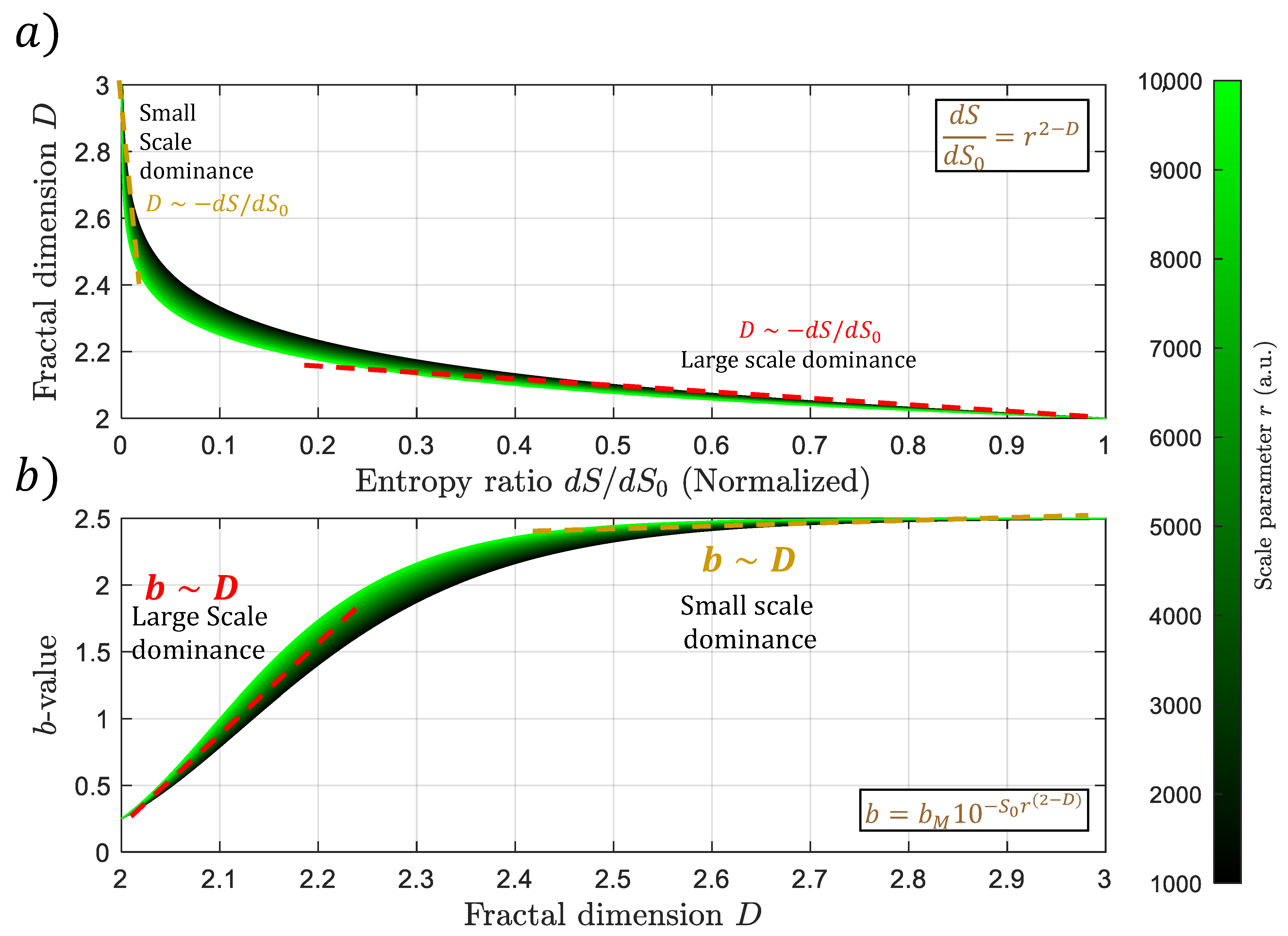
• Multiscale thermodynamics indicates that the b-value is proportional to the thermodynamic fractal dimension $D$ when either small-scale or large-scale energy dissipation dominates. This implies that the decreases in the b-value indicate the lithosphere is preparing to release energy macroscopically.
• The existence of small-scale dynamics within rocks plays a critical role in the multiscale cracking process and the generation of electromagnetic signals before earthquakes. This indicates that earthquakes can be triggered without evident large-scale stress changes.
• The electrification of rocks on a large scale can be achieved through two mechanisms: it can be directly proportional to the macroscopic stress change or inversely related to the microscopic stress. Therefore, when small-scale stress changes are reduced, it results in the generation of macroscopic electric currents.
• Future research endeavors should aim to establish a connection between the impact of small-scale dynamics and fault characteristics, such as the seismic moment, earthquake magnitude, or fault’s smoothness processes.

References

1. Mishnaevsky, L. Methods of the theory of complex systems in modelling of fracture: A brief review. Eng. Fract. Mech. 1997, 56, 47–56. [Google Scholar] [CrossRef]
2. Ansell, H.; Blom, A. Fatigue: Damage Tolerance Design. Encycl. Mater. Sci. Technol. 2016, 1, 2906–2910. [Google Scholar] [CrossRef]
3. Han, X.; Xiao, Q.; Cui, K.; Hu, X.; Chen, Q.; Li, C.; Qiu, Z. Predicting the fracture behavior of concrete using artificial intelligence approaches and closed-form solution. Theor. Appl. Fract. Mech. 2021, 112, 102892. [Google Scholar] [CrossRef]
4. Biswas, S.; Goehring, L.; Chakrabarti, B.K. Statistical physics of fracture and earthquakes. Philos. Trans. R. Soc. A Math. Phys. Eng. Sci. 2018, 377, 20180202. [Google Scholar] [CrossRef] [Green Version]
5. Clerc, G.; Brunner, A.J.; Niemz, P.; van de Kuilen, J.-W. Application of fracture mechanics to engineering design of complex structures. Procedia Struct. Integr. 2020, 28, 1761–1767. [Google Scholar] [CrossRef]
6. Taylor, D.; O’brien, F.; Lee, T. A Theoretical Model for the Simulation of Microdamage Accumulation and Repair in Compact Bone. Meccanica 2002, 37, 397–406. [Google Scholar] [CrossRef]
7. O’brien, F.J.; Brennan, O.; Kennedy, O.D.; Lee, T.C. Microcracks in cortical bone: How do they affect bone biology? Curr. Osteoporos. Rep. 2005, 3, 39–45. [Google Scholar] [CrossRef]
8. Tisbo, P.; Taylor, D. Simulation of Microcrack Growth and Repair in Living Bone. WIT Trans. Biomed. Health 2013, 17, 193–203. [Google Scholar] [CrossRef] [Green Version]
9. Enomoto, Y.; Hashimoto, H. Emission of charged particles from indentation fracture of rocks. Nature 1990, 346, 641–643. [Google Scholar] [CrossRef]
10. Xie, H. Fractals in Rock Mechanics, 1st ed.; CRC Press: Boca Raton, FL, USA, 1993. [Google Scholar]
11. Hsieh, A.; Dyskin, A.; Dight, P. The increase in Young׳s modulus of rocks under uniaxial compression. Int. J. Rock Mech. Min. Sci. 2014, 70, 425–434. [Google Scholar] [CrossRef] [Green Version]
12. Molent, L.; Spagnoli, A.; Carpinteri, A.; Jones, R. Using the lead crack concept and fractal geometry for fatigue lifing of metallic structural components. Int. J. Fatigue 2017, 102, 214–220. [Google Scholar] [CrossRef]
13. Chen, C.-F.; Xu, T.; Li, S.-H. Microcrack Evolution and Associated Deformation and Strength Properties of Sandstone Samples Subjected to Various Strain Rates. Minerals 2018, 8, 231. [Google Scholar] [CrossRef] [Green Version]
14. Cartwright-Taylor, A.; Main, I.G.; Butler, I.B.; Fusseis, F.; Flynn, M.; King, A. Catastrophic Failure: How and When? Insights From 4-D In Situ X-ray Microtomography. J. Geophys. Res. Solid Earth 2020, 125, e2020JB019642. [Google Scholar] [CrossRef]
15. Isah, B.W.; Mohamad, H.; Ahmad, N.R.; Harahap, I.S.H.; Al-Bared, M.A.M. Uniaxial compression test of rocks: Review of strain measuring instruments. IOP Conf. Ser. Earth Environ. Sci. 2020, 476, 012039. [Google Scholar] [CrossRef]
16. McBeck, J.; Ben-Zion, Y.; Renard, F. Fracture Network Localization Preceding Catastrophic Failure in Triaxial Compression Experiments on Rocks. Front. Earth Sci. 2021, 9, 778811. [Google Scholar] [CrossRef]
17. Mao, W.; Wu, L.; Xu, Y.; Yao, R.; Lu, J.; Sun, L.; Qi, Y. Pressure-Stimulated Rock Current as Loading Diorite to Failure: Particular Variation and Holistic Mechanisms. J. Geophys. Res. Solid Earth 2022, 127, e2022JB024931. [Google Scholar] [CrossRef]
18. Triantis, D.; Pasiou, E.D.; Stavrakas, I.; Kourkoulis, S.K. Hidden Affinities Between Electric and Acoustic Activities in Brittle Materials at Near-Fracture Load Levels. Rock Mech. Rock Eng. 2022, 55, 1325–1342. [Google Scholar] [CrossRef]
19. Guo, J.; Yu, L.; Wen, Z.; Feng, G.; Bai, J.; Wen, X.; Qi, T.; Qian, R.; Zhu, L.; Guo, X.; et al. Mechanical and Acoustic Emission Characteristics of Coal-like Rock Specimens under Static Direct Shear and Dynamic Normal Load. Materials 2022, 15, 6546. [Google Scholar] [CrossRef]
20. Costa, J.P.M.; Jumel, J. Theoretical analysis of self-similar crack propagation along viscoelastic and elasto–viscoplastic interface in a double cantilever beam test. Int. J. Fract. 2023, 1, 1–17. [Google Scholar] [CrossRef]
21. Stavrakas, I.; Triantis, D.; Agioutantis, Z.; Maurigiannakis, S.; Saltas, V.; Vallianatos, F.; Clarke, M. Pressure stimulated currents in rocks and their correlation with mechanical properties. Nat. Hazards Earth Syst. Sci. 2004, 4, 563–567. [Google Scholar] [CrossRef] [Green Version]
22. Pasiou, E.D.; Triantis, D. Correlation between the electric and acoustic signals emitted during compression of brittle materials. Frat. Ed Integrità Strutt. 2017, 11, 41–51. [Google Scholar] [CrossRef] [Green Version]
23. Li, D.; Wang, E.; Li, Z.; Ju, Y.; Wang, D.; Wang, X. Experimental investigations of pressure stimulated currents from stressed sandstone used as precursors to rock fracture. Int. J. Rock Mech. Min. Sci. 2021, 145, 104841. [Google Scholar] [CrossRef]
24. Anastasiadis, C.; Stavrakas, I.; Triantis, D.; Vallianatos, F. Correlation of pressure stimulated currents in rocks with the damage parameter. Ann. Geophys. 2009, 50, 1–6. [Google Scholar] [CrossRef]
25. Stroh, A.N. The formation of cracks in plastic flow. II. Proc. R. Soc. London. Ser. A Math. Phys. Sci. 1955, 232, 548–560. [Google Scholar] [CrossRef]
26. Slifkin, L. Seismic electric signals from displacement of charged dislocations. Tectonophysics 1993, 224, 149–152. [Google Scholar] [CrossRef]
27. Vallianatos, F.; Tzanis, A. Electric current generation associated with the deformation rate of a solid: Preseismic and coseismic signals. Phys. Chem. Earth 1998, 23, 933–938. [Google Scholar] [CrossRef]
28. Vallianatos, F.; Tzanis, A. On the nature, scaling and spectral properties of pre-seismic ULF signals. Nat. Hazards Earth Syst. Sci. 2003, 3, 237–242. [Google Scholar] [CrossRef]
29. Venegas-Aravena, P.; Cordaro, E.G.; Laroze, D. A review and upgrade of the lithospheric dynamics in context of the seismo-electromagnetic theory. Nat. Hazards Earth Syst. Sci. 2019, 19, 1639–1651. [Google Scholar] [CrossRef] [Green Version]
30. Agalianos, G.; Tzagkarakis, D.; Loukidis, A.; Pasiou, E.D.; Triantis, D.; Kourkoulis, S.K.; Stavrakas, I. Correlation of Acoustic Emissions and Pressure Stimulated Currents recorded in Alfas-stone specimens under three-point bending. The role of the specimens’ porosity: Preliminary results. 2nd Mediterranean Conference on Fracture and Structural Integrity. Procedia Struct. Integr. 2022, 41, 452–460. [Google Scholar] [CrossRef]
31. Lin, P.; Wei, P.; Wang, C.; Kang, S.; Wang, X. Effect of rock mechanical properties on electromagnetic radiation mechanism of rock fracturing. J. Rock Mech. Geotech. Eng. 2021, 13, 798–810. [Google Scholar] [CrossRef]
32. Scoville, J.; Heraud, J.; Freund, F. Pre-earthquake magnetic pulses. Nat. Hazards Earth Syst. Sci. 2015, 15, 1873–1880. [Google Scholar] [CrossRef] [Green Version]
33. Schekotov, A.; Hayakawa, M. Seismo-meteo-electromagnetic phenomena observed during a 5-year interval around the 2011 Tohoku earthquake. Phys. Chem. Earth Parts A/B/C 2015, 85, 167–173. [Google Scholar] [CrossRef]
34. Enomoto, Y.; Yamabe, T.; Okumura, N. Causal mechanisms of seismo-EM phenomena during the 1965–1967 Matsushiro earthquake swarm. Sci. Rep. 2017, 7, srep44774. [Google Scholar] [CrossRef] [Green Version]
35. De Santis, A.; Balasis, G.; Pavón-Carrasco, F.; Cianchini, G.; Mandea, M. Potential earthquake precursory pattern from space: The 2015 Nepal event as seen by magnetic Swarm satellites. Earth Planet. Sci. Lett. 2017, 461, 119–126. [Google Scholar] [CrossRef] [Green Version]
36. Potirakis, S.M.; Hayakawa, M.; Schekotov, A. Fractal analysis of the ground-recorded ULF magnetic fields prior to the 11 March 2011 Tohoku earthquake (M W = 9): Discriminating possible earthquake precursors from space-sourced disturbances. Nat. Hazards 2016, 85, 59–86. [Google Scholar] [CrossRef]
37. Cordaro, E.G.; Venegas, P.; Laroze, D. Latitudinal variation rate of geomagnetic cutoff rigidity in the active Chilean convergent margin. Ann. Geophys. 2018, 36, 275–285. [Google Scholar] [CrossRef] [Green Version]
38. De Santis, A.; Marchetti, D.; Pavón-Carrasco, F.J.; Cianchini, G.; Perrone, L.; Abbattista, C.; Alfonsi, L.; Amoruso, L.; Campuzano, S.A.; Carbone, M.; et al. Precursory worldwide signatures of earthquake occurrences on Swarm satellite data. Sci. Rep. 2019, 9, 20287. [Google Scholar] [CrossRef] [Green Version]
39. Cordaro, E.G.; Venegas-Aravena, P.; Laroze, D. Long-term magnetic anomalies and their possible relationship to the latest greater Chilean earthquakes in the context of the seismo-electromagnetic theory. Nat. Hazards Earth Syst. Sci. 2021, 21, 1785–1806. [Google Scholar] [CrossRef]
40. De Santis, A.; Perrone, L.; Calcara, M.; Campuzano, S.; Cianchini, G.; D’arcangelo, S.; Di Mauro, D.; Marchetti, D.; Nardi, A.; Orlando, M.; et al. A comprehensive multiparametric and multilayer approach to study the preparation phase of large earthquakes from ground to space: The case study of the June 15 2019, M7.2 Kermadec Islands (New Zealand) earthquake. Remote. Sens. Environ. 2022, 283, 113325. [Google Scholar] [CrossRef]
41. Venegas-Aravena, P.; Cordaro, E.G.; Laroze, D. The spatial–temporal total friction coefficient of the fault viewed from the perspective of seismo-electromagnetic theory. Nat. Hazards Earth Syst. Sci. 2020, 20, 1485–1496. [Google Scholar] [CrossRef]
42. Venegas-Aravena, P.; Cordaro, E.G.; Laroze, D. Entropy Approach from Cracks in the Semi Brittle-Ductile Lithosphere and Generalization. Entropy 2022, 24, 1337. [Google Scholar] [CrossRef]
43. Venegas-Aravena, P.; Cordaro, E.; Laroze, D. Fractal Clustering as Spatial Variability of Magnetic Anomalies Measurements for Impending Earthquakes and the Thermodynamic Fractal Dimension. Fractal Fract. 2022, 6, 624. [Google Scholar] [CrossRef]
44. Marzocchi, W.; Sandri, L. A review and new insights on the estimation of the b-valueand its uncertainty. Ann. Geophys. 2009, 46, 1271–1282. [Google Scholar] [CrossRef]
45. Scholz, C.H. On the stress dependence of the earthquake b value. Geophys. Res. Lett. 2015, 42, 1399–1402. [Google Scholar] [CrossRef] [Green Version]
46. Weeks, J.; Lockner, D.; Byerlee, J. Change in b-values during movement on cut surfaces in granite. Bull. Seism. Soc. Am. 1978, 68, 333–341. [Google Scholar] [CrossRef]
47. Colombo, I.S.; Main, I.G.; Forde, M.C. Assessing Damage of Reinforced Concrete Beam Using “b-value” Analysis of Acoustic Emission Signals. J. Mater. Civ. Eng. 2003, 15, 280–286. [Google Scholar] [CrossRef] [Green Version]
48. Guzmán, C.; Torres, D.; Hucailuk, C.; Filipussi, D. Analysis of the Acoustic Emission in a Reinforced Concrete Beam Using a Four Points Bending Test. Procedia Mater. Sci. 2015, 8, 148–154. [Google Scholar] [CrossRef] [Green Version]
49. Main, I.G. Damage mechanics with long-range interactions: Correlation between the seismic b-value and the fractal two-point correlation dimension. Geophys. J. Int. 1992, 111, 531–541. [Google Scholar] [CrossRef] [Green Version]
50. Rao, M.V.M.S.; Lakshmi, K.J.P. Analysis of b-value and improved b-value of acoustic emissions accompanying rock fracture. Curr. Sci. 2005, 89, 1577–1582. Available online: http://www.jstor.org/stable/24110936 (accessed on 1 June 2023).
51. Loukidis, A.; Tzagkarakis, D.; Kyriazopoulos, A.; Stavrakas, I.; Triantis, D. Correlation of Acoustic Emissions with Electrical Signals in the Vicinity of Fracture in Cement Mortars Subjected to Uniaxial Compressive Loading. Appl. Sci. 2022, 13, 365. [Google Scholar] [CrossRef]
52. Dong, L.; Zhang, L.; Liu, H.; Du, K.; Liu, X. Acoustic Emission b Value Characteristics of Granite under True Triaxial Stress. Mathematics 2022, 10, 451. [Google Scholar] [CrossRef]
53. Tzanis, A.; Vallianatos, F. A physical model of electrical earthquake precursors due to crack propagation and the motion of charged edge dislocations, in: Seismo Electromagnetics (Lithosphere–Atmosphere–Ionosphere-Coupling). TerraPub 2002, 1, 117–130. [Google Scholar]
54. Anastasiadis, C.; Triantis, D.; Stavrakas, I.; Vallianatos, F. Pressure Stimulated Currents (PSC)in marble samples. Ann. Geophys. 2009, 47, 21–28. [Google Scholar] [CrossRef]
55. Onsager, L. Reciprocal Relations in Irreversible Processes. I. Phys. Rev. 1931, 37, 405–426. [Google Scholar] [CrossRef] [Green Version]
56. Onsager, L. Reciprocal Relations in Irreversible Processes. II. Phys. Rev. 1931, 38, 2265–2279. [Google Scholar] [CrossRef] [Green Version]
57. Hirata, T.; Satoh, T.; Ito, K. Fractal structure of spatial distribution of microfracturing in rock. Geophys. J. Int. 1987, 90, 369–374. [Google Scholar] [CrossRef]
58. De Santis, A.; Cianchini, G.; Favali, P.; Beranzoli, L.; Boschi, E. The Gutenberg-Richter Law and Entropy of Earthquakes: Two Case Studies in Central Italy. Bull. Seism. Soc. Am. 2011, 101, 1386–1395. [Google Scholar] [CrossRef]
59. Kranz, R.L. Microcracks in rocks: A review. Tectonophysics 1983, 100, 449–480. [Google Scholar] [CrossRef]
60. Chen, H.; Han, P.; Hattori, K. Recent Advances and Challenges in the Seismo-Electromagnetic Study: A Brief Review. Remote Sens. 2022, 14, 5893. [Google Scholar] [CrossRef]
61. Dey, C.; Baruah, S.; Rawat, G.; Chetia, T.; Baruah, S.; Sharma, S. Appraisal of contemporaneous application of polarization ratio and fractal analysis for studying possible seismo-electromagnetic emissions during an intense phase of seismicity in and around Assam Valley and the Eastern Himalayas, India. Phys. Earth Planet. Inter. 2021, 318, 106759. [Google Scholar] [CrossRef]
62. D’incecco, S.; Petraki, E.; Priniotakis, G.; Papoutsidakis, M.; Yannakopoulos, P.; Nikolopoulos, D. CO2 and Radon Emissions as Precursors of Seismic Activity. Earth Syst. Environ. 2021, 5, 655–666. [Google Scholar] [CrossRef]
63. Feng, L.; Qu, R.; Ji, Y.; Zhu, W.; Zhu, Y.; Feng, Z.; Fan, W.; Guan, Y.; Xie, C. Multistationary Geomagnetic Vertical Intensity Polarization Anomalies for Predicting M ≥ 6 Earthquakes in Qinghai, China. Appl. Sci. 2022, 12, 8888. [Google Scholar] [CrossRef]
64. Florios, K.; Contopoulos, I.; Christofilakis, V.; Tatsis, G.; Chronopoulos, S.; Repapis, C.; Tritakis, V. Pre-seismic Electromagnetic Perturbations in Two Earthquakes in Northern Greece. Pure Appl. Geophys. 2019, 177, 787–799. [Google Scholar] [CrossRef]
65. Huang, J.; Wang, Q.; Yan, R.; Lin, J.; Zhao, S.; Chu, W.; Shen, X.; Zeren, Z.; Yang, Y.; Cui, J.; et al. Pre-seismic multi-parameters variations before Yangbi and Madoi earthquakes on May 21, 2021. Nat. Hazards Res. 2023, 3, 27–34. [Google Scholar] [CrossRef]
66. Weiyu, M.; Xuedong, Z.; Liu, J.; Yao, Q.; Zhou, B.; Yue, C.; Kang, C.; Lu, X. Influences of multiple layers of air temperature differences on tidal forces and tectonic stress before, during and after the Jiujiang earthquake. Remote Sens. Environ. 2018, 210, 159–165. [Google Scholar] [CrossRef]
67. Petraki, E.; Nikolopoulos, D.; Nomicos, C.; Stonham, J.; Cantzos, D.; Yannakopoulos, P.; Kottou, S. Electromagnetic Pre-earthquake Precursors: Mechanisms, Data and Models—A Review. J. Earth Sci. Clim. Chang. 2015, 6, 250. [Google Scholar] [CrossRef] [Green Version]
68. Sorokin, V.; Yaschenko, A.; Mushkarev, G.; Novikov, V. Telluric Currents Generated by Solar Flare Radiation: Physical Model and Numerical Estimations. Atmosphere 2023, 14, 458. [Google Scholar] [CrossRef]
69. Vargas, C.A.; Gomez, J.S.; Gomez, J.J.; Solano, J.M.; Caneva, A. Space–Time Variations of the Apparent Resistivity Associated with Seismic Activity by Using 1D-Magnetotelluric (MT) Data in the Central Part of Colombia (South America). Appl. Sci. 2023, 13, 1737. [Google Scholar] [CrossRef]
70. Sigalotti, L.D.G.; Ramírez-Rojas, A.; Vargas, C.A. Tsallis q-Statistics in Seismology. Entropy 2023, 25, 408. [Google Scholar] [CrossRef]
71. Gunarathna, G.; da Silva, B.G. Effect of the Triaxial State of Stress in the Hydraulic Fracturing Processes of Granite: Part 1—Visual Observations and Interpretation. Rock Mech. Rock Eng. 2021, 54, 2903–2923. [Google Scholar] [CrossRef]
72. Göğüş, D.; Avşar, E. Stress levels of precursory strain localization subsequent to the crack damage threshold in brittle rock. PLoS ONE 2022, 17, e0276214. [Google Scholar] [CrossRef]
73. Shams, G.; Rivard, P.; Moradian, O. Micro-scale Fracturing Mechanisms in Rocks During Tensile Failure. Rock Mech. Rock Eng. 2023, 1, 1–23. [Google Scholar] [CrossRef]
74. Borla, O.; Lacidogna, G.; Di Battista, E.; Niccolini, G.; Carpinteri, A. Electromagnetic Emission as Failure Precursor Phenomenon for Seismic Activity Monitoring. In Fracture, Fatigue, Failure, and Damage Evolution, Volume 5: Conference Proceedings of the Society for Experimental Mechanics Series; Carroll, J., Daly, S., Eds.; Springer: Cham, Switzerland, 2015. [Google Scholar] [CrossRef]
75. Niccolini, G.; Potirakis, S.M.; Lacidogna, G.; Borla, O. Criticality Hidden in Acoustic Emissions and in Changing Electrical Resistance during Fracture of Rocks and Cement-Based Materials. Materials 2020, 13, 5608. [Google Scholar] [CrossRef]
76. Chen, X.; Li, Y.; Chen, L. The characteristics of the b-value anomalies preceding the 2004 Mw9.0 Sumatra earthquake. Geomat. Nat. Hazards Risk 2022, 13, 390–399. [Google Scholar] [CrossRef]
77. Klyuchkin, V.N.; Novikov, V.A.; Okunev, V.I.; Zeigarnik, V.A. Acoustic and electromagnetic emissions of rocks: Insight from laboratory tests at press and shear machines. Environ. Earth Sci. 2022, 81, 64. [Google Scholar] [CrossRef]
78. Brantut, N.; Schubnel, A.; David, E.C.; Héripré, E.; Guéguen, Y.; Dimanov, A. Dehydration-induced damage and deformation in gypsum and implications for subduction zone processes. J. Geophys. Res. Atmos. 2012, 117. [Google Scholar] [CrossRef] [Green Version]
79. Hough, S.E. Predicting the Unpredictable: The Tumultuous Science of Earthquake Prediction; Princeton University Press: Princeton, NJ, USA, 2010. [Google Scholar]
80. Marinescu, I.D.; Pruteanu, M. Chapter 2—Deformation and Fracture of Ceramic Materials in Handbook of Ceramics Grinding and Polishing, 2nd ed.; William Andrew Publishing: Norwich, NY, USA, 2015; pp. 50–66. [Google Scholar] [CrossRef]
81. Bryant, M.D. Entropy and Dissipative Processes of Friction and Wear. FME Trans. 2009, 37, 55–60. [Google Scholar]
82. Nielsen, S.; Spagnuolo, E.; Violay, M.; Smith, S.; Di Toro, G.; Bistacchi, A. G: Fracture energy, friction and dissipation in earthquakes. J. Seism. 2016, 20, 1187–1205. [Google Scholar] [CrossRef] [Green Version]
Figure 1. The experimental setup is schematically represented, where the applied stress is considered almost constant, and despite this, electromagnetic and acoustic emissions can be observed from microcracks.
Geosciences 13 00169 g001
Figure 2. A study was conducted to analyze the relationship between the thermodynamic fractal dimension D , the b-value, the balance of entropy changes Ω V = ω 0 d S d S 0 (for ω 0 = 1), and the scaling factor r through parameterization. (a) Equation (7) shows a negative correlation between the fractal dimension and the entropy balance Ω V . However, for two regimes (indicated by red and dark yellow dashed lines), this relationship tends to be almost linear. This suggests that when the large- and small-scale entropy change dominates the system, the fractal dimension tends to be small (<2.2) for a system governed by large-scale entropy (large Ω V ). (b) When the fractal dimension is small, as in the above scenario, there is an almost linear relationship between b and D (indicated by the red dashed line). The relationship between the thermodynamic fractal dimension D , the b-value, and the balance of entropy changes Ω V . (a) Equation (7) shows a negative correlation between the fractal dimension and the entropy balance Ω V , with two regimes showing an almost linear relationship (red and dark yellow dashed lines). (b) A small fractal dimension (<2.2) corresponds to large-scale entropy in the system. In this scenario, there is an almost linear relationship between b and D , as indicated by the red dashed line.
Geosciences 13 00169 g002
Figure 3. (a) Relationship between electromagnetic signals, b-value, and entropy change balance. The b-value decreases as the entropy change ( d S ) increases, while the electromagnetic signals increase, as indicated by the green and red curves. (b) The schematic shows the evolution of stress (represented by a black constant line) and the negative relationship between the b-value (represented by a red line) and the electromagnetic emissions (represented by a blue line).
Geosciences 13 00169 g003
Figure 4. (a) A simplified depiction of the pulse-like behavior of b-value and electromagnetic signals discovered by Loukidis et al. [51] is shown with the red and blue curves, respectively. The b-value is computed using Equation (15). (b) The stress change balance Ω σ ˙ required to observe the pulse-like behavior of (a) is illustrated. The magenta curve denotes the nearly zero external applied stress change ( σ = 0.001 a.u.). Note that this curve is normalized. The red line represents the microscopic stress that must be evolving for the pulse-like behavior of b and J ^ e with an almost constant macroscopic applied stress. (c) A schematic representation of the small-scale dominance entropy production is displayed. Most of the system is filled with small-scale cracks. This is equivalent to t = 0 a.u. in (a,b). (d) A schematic representation of large-scale dominance of entropy production is presented. In this scenario, the system is filled with large-scale cracks. This scenario represents the case when the small-scale entropy production is minimal. That is, when t = 0.5 a.u. in (a,b).
Geosciences 13 00169 g004
Disclaimer/Publisher’s Note: The statements, opinions and data contained in all publications are solely those of the individual author(s) and contributor(s) and not of MDPI and/or the editor(s). MDPI and/or the editor(s) disclaim responsibility for any injury to people or property resulting from any ideas, methods, instructions or products referred to in the content.