
Commentary and Review of Modern Environmental Problems Linked to Historic Flow Capacity in Arid Groundwater Basins

Abstract
:1. Introduction
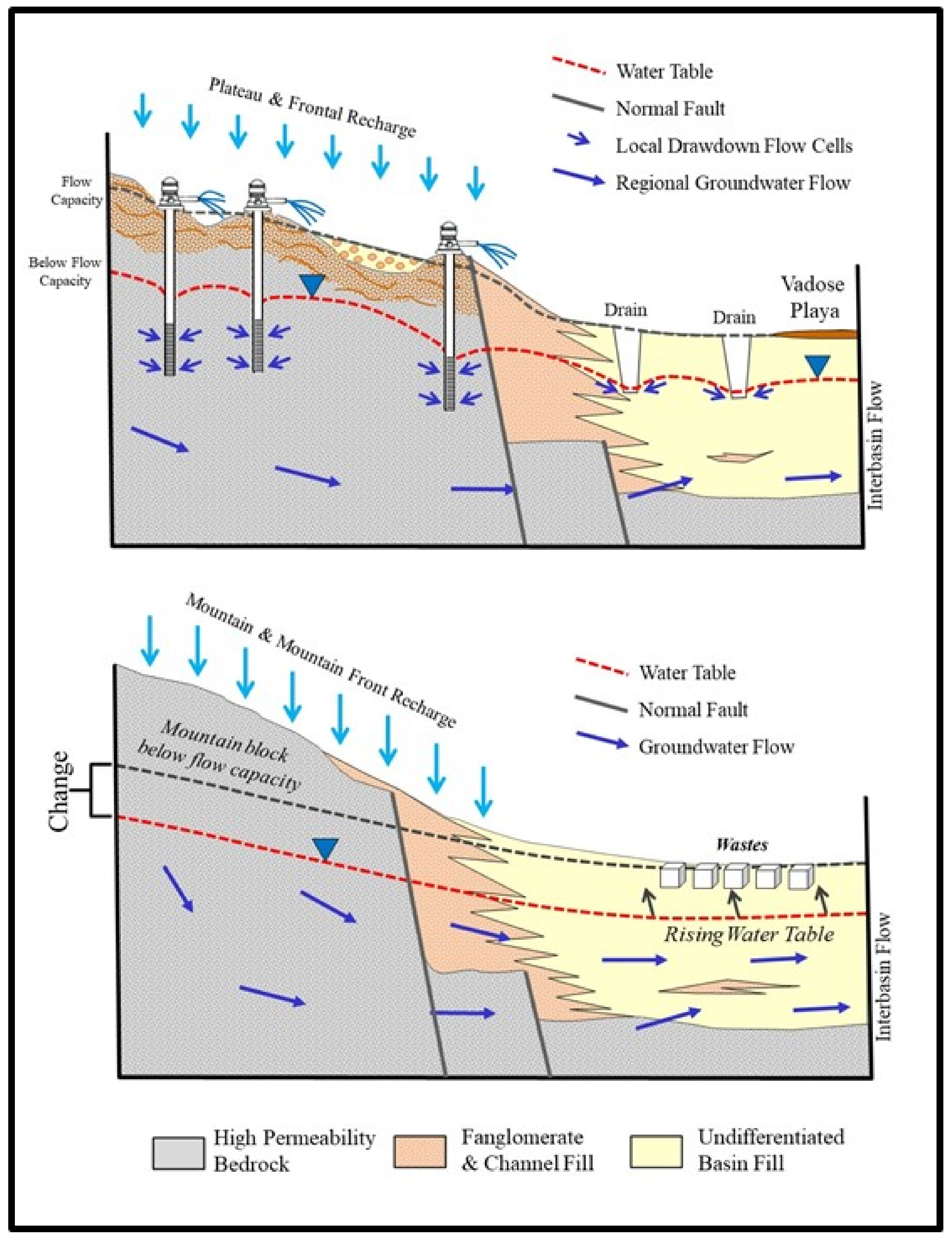
1.1. Previous Research on Aquifer Flow Capacity
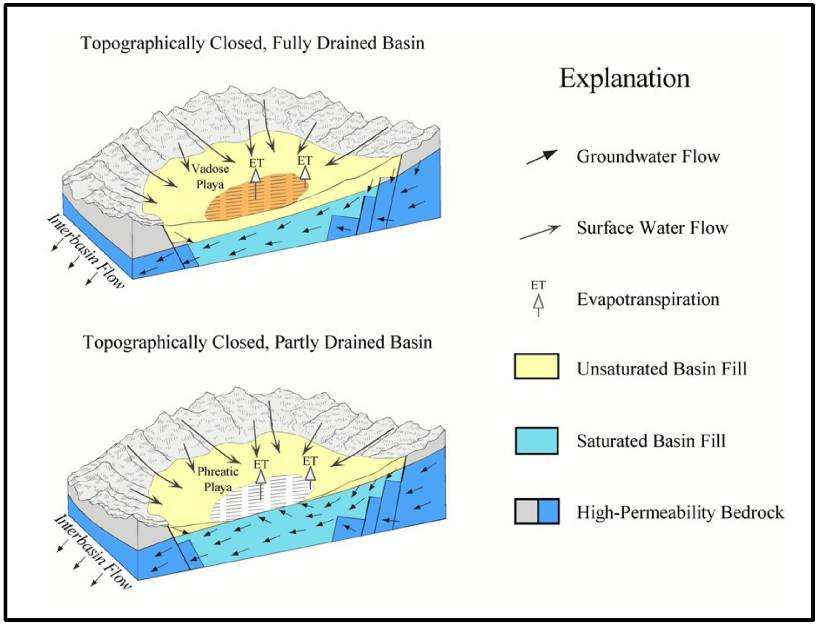
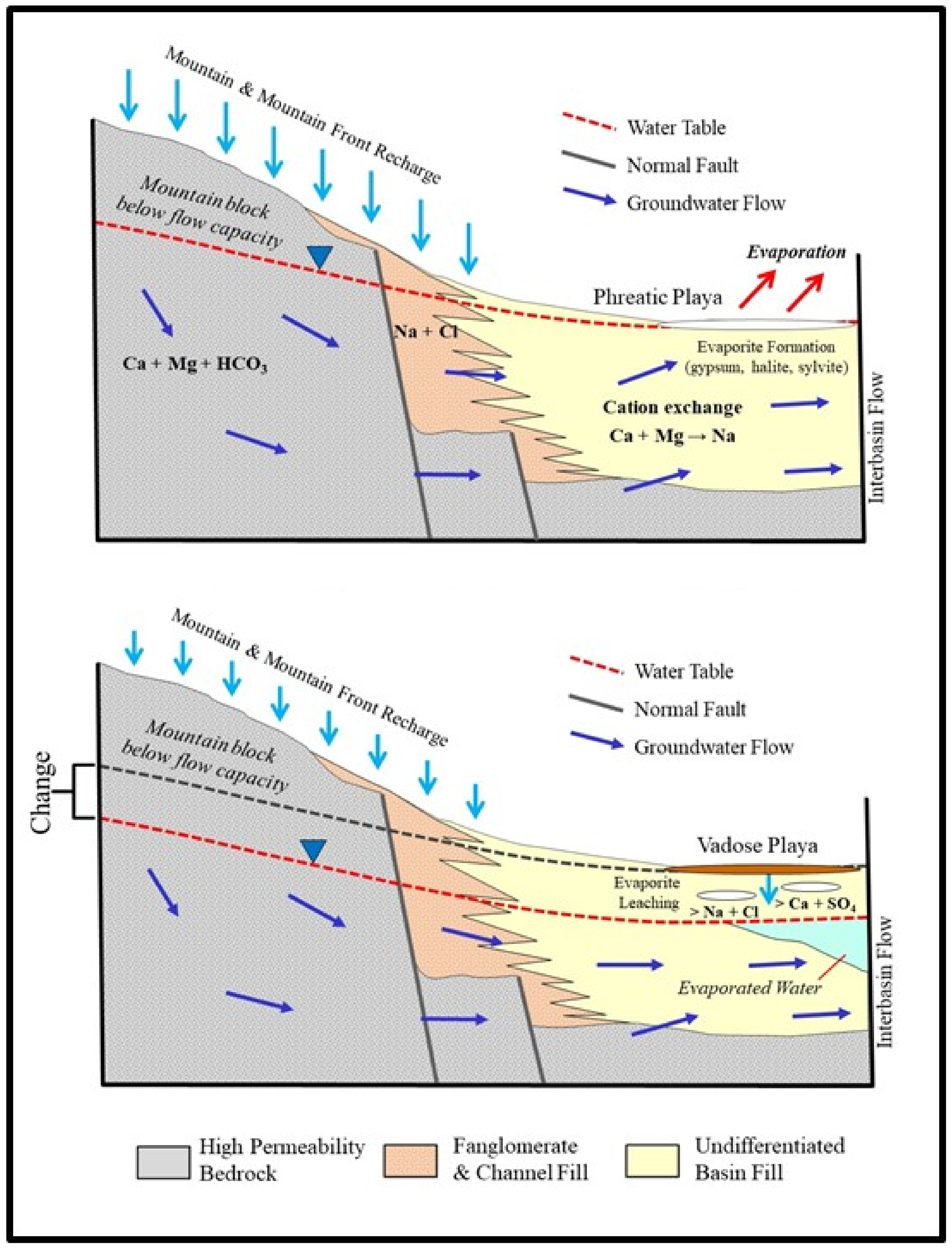
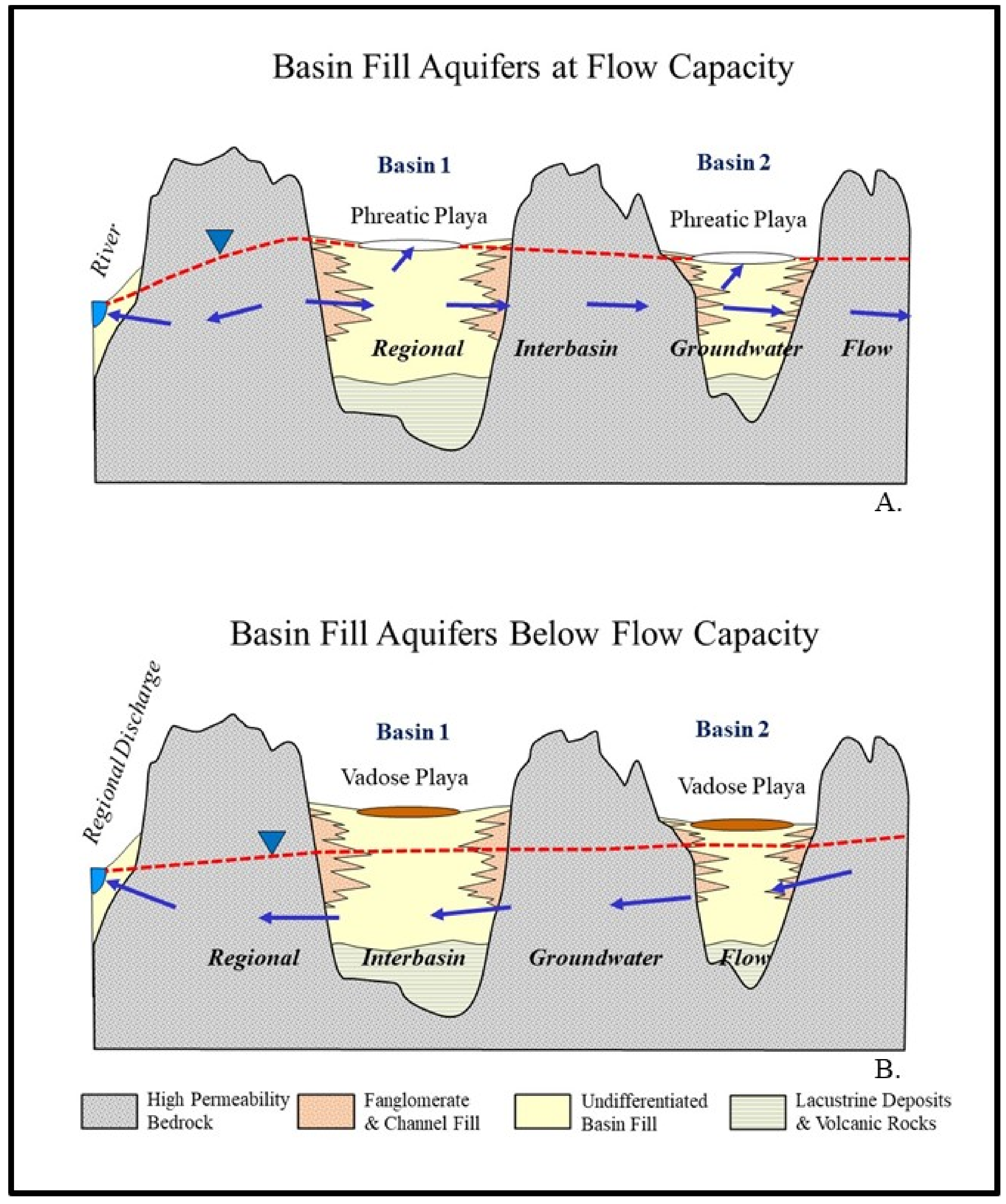
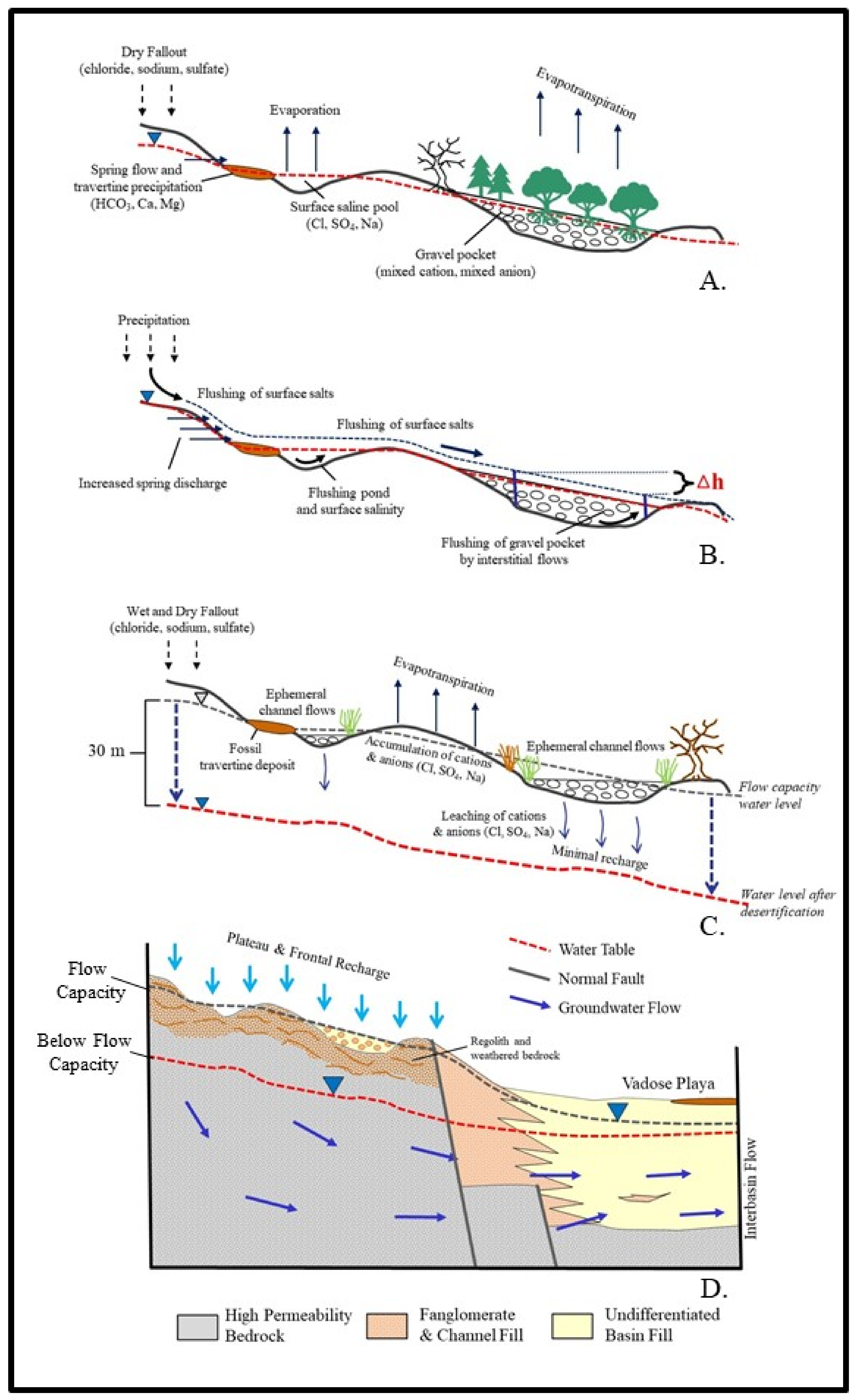
1.2. Relationship of Flow Capacity to Internal Playas in Groundwater Basins
2. Methods

| Topic | Case Example | Case Example: Source, Data, or Findings |
|---|---|---|
| 3.1. Flow Capacity and Aquifer Water Levels | Example 1. Paleo Spring Discharge in Death Valley, USA | Miner et al. [13] |
| 3.2. Flow Capacity and Groundwater Salinity | Example 2. Paleoclimate and Salinity of Ivanpah Valley, USA | Waring, [25]; Sims and Spaulding, [26]; This Paper |
| 3.3. Flow Capacity and Toxic Trace Elements | Example 3. Arsenic Loading to Ground- water from a Drained Phreatic Playa— San Diego Creek Watershed, USA | Hibbs and Andrus, [34] |
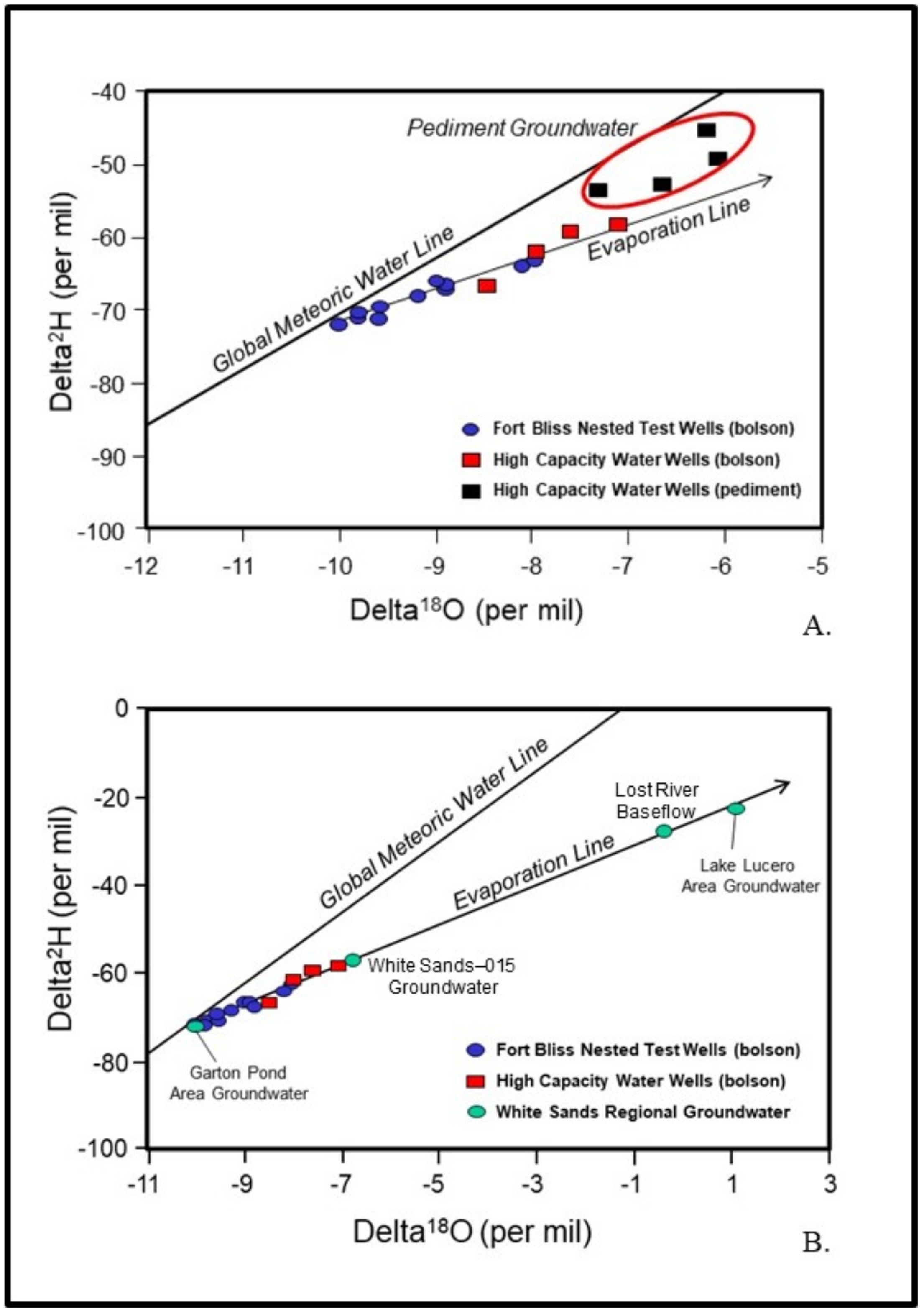
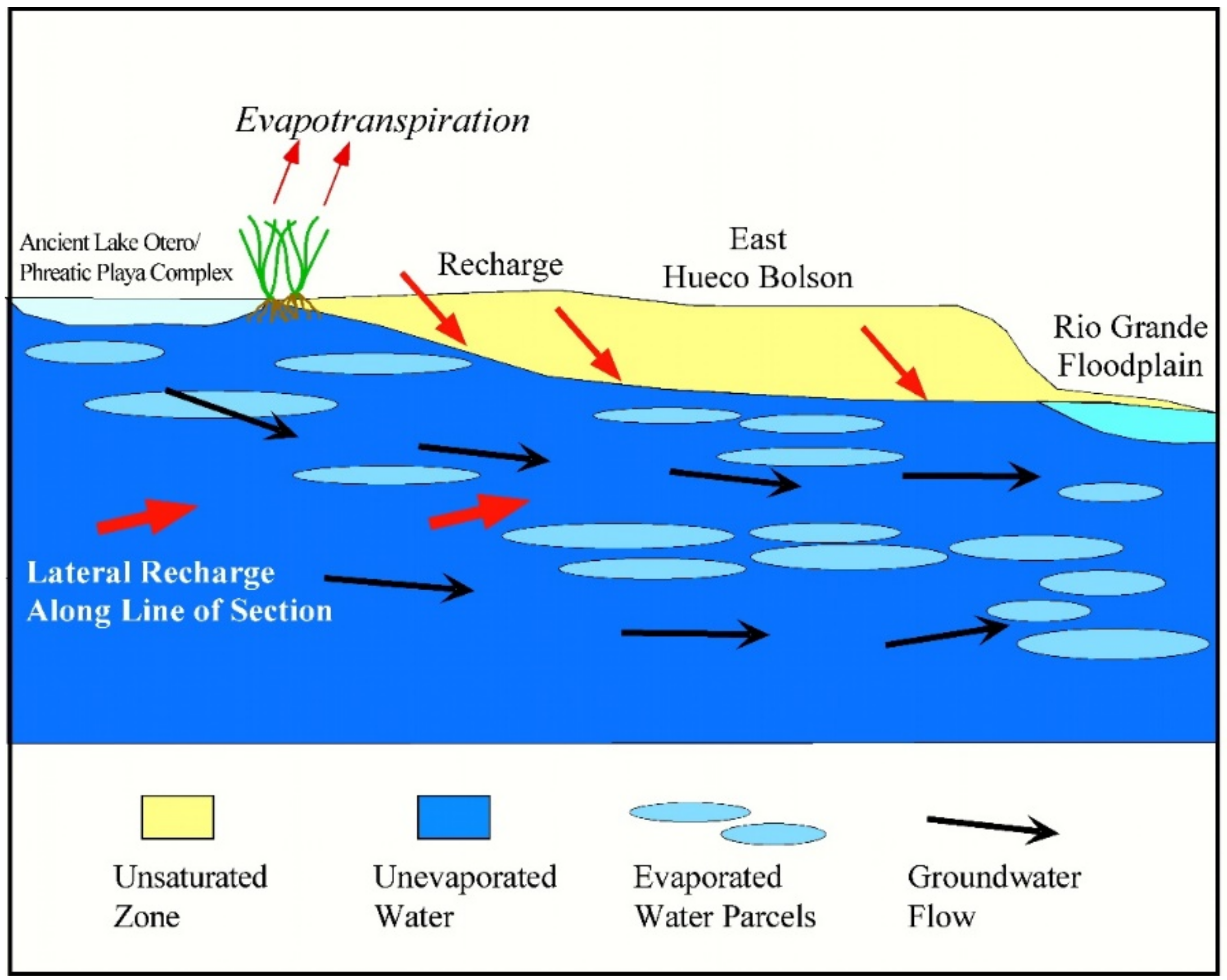
| 3.4. Isotope Hydrology and Flow Capacity | Example 4. Isotopically Evaporated Water in Eastern Hueco Bolson, USA | Hibbs and Ortiz, in press Newton and Allen, [35] |
| 3.5. Flow Capacity, Fossil Hydraulic Gradients, and Groundwater Modeling | Example 5. Variable Density Modeling of Groundwater Flow near a Phreatic Playa | Duffy and Al-Hassan, 1988 Hamann et al. [27,28] |
3. Topics and Case Examples Related to Aquifer Flow Capacity and Paleoclimate and Anthropogenic Change
3.1. Flow Capacity and Aquifer Water Levels
Case Example 1—Paleospring Discharge in Death Valley, USA
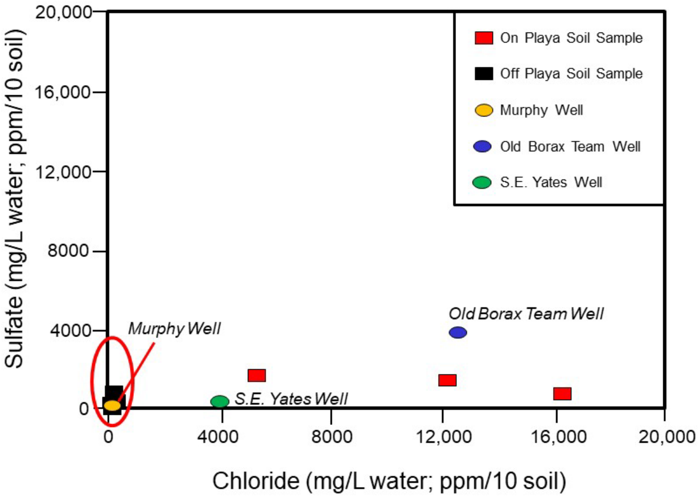
3.2. Flow Capacity and Groundwater Salinity
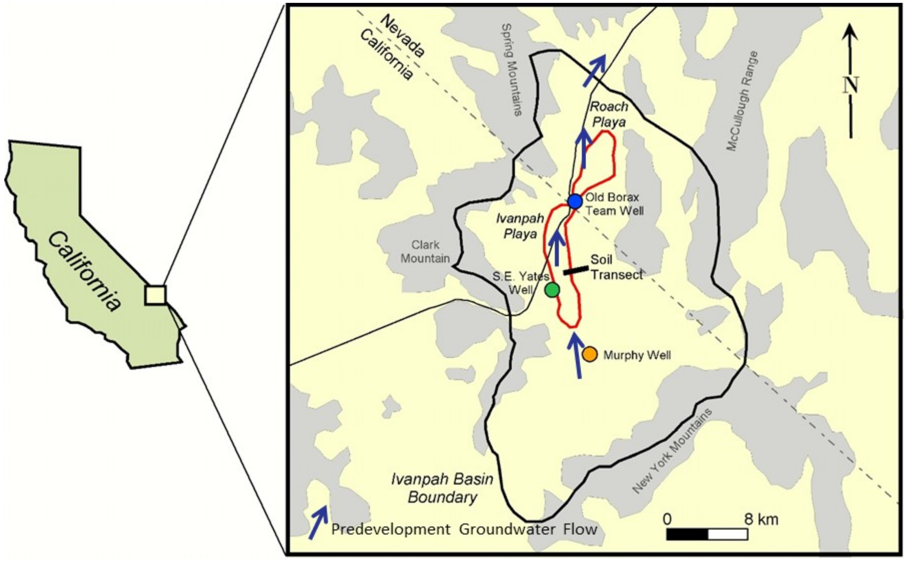
Case Example 2—Paleoclimate and Salinity of Ivanpah Valley, USA
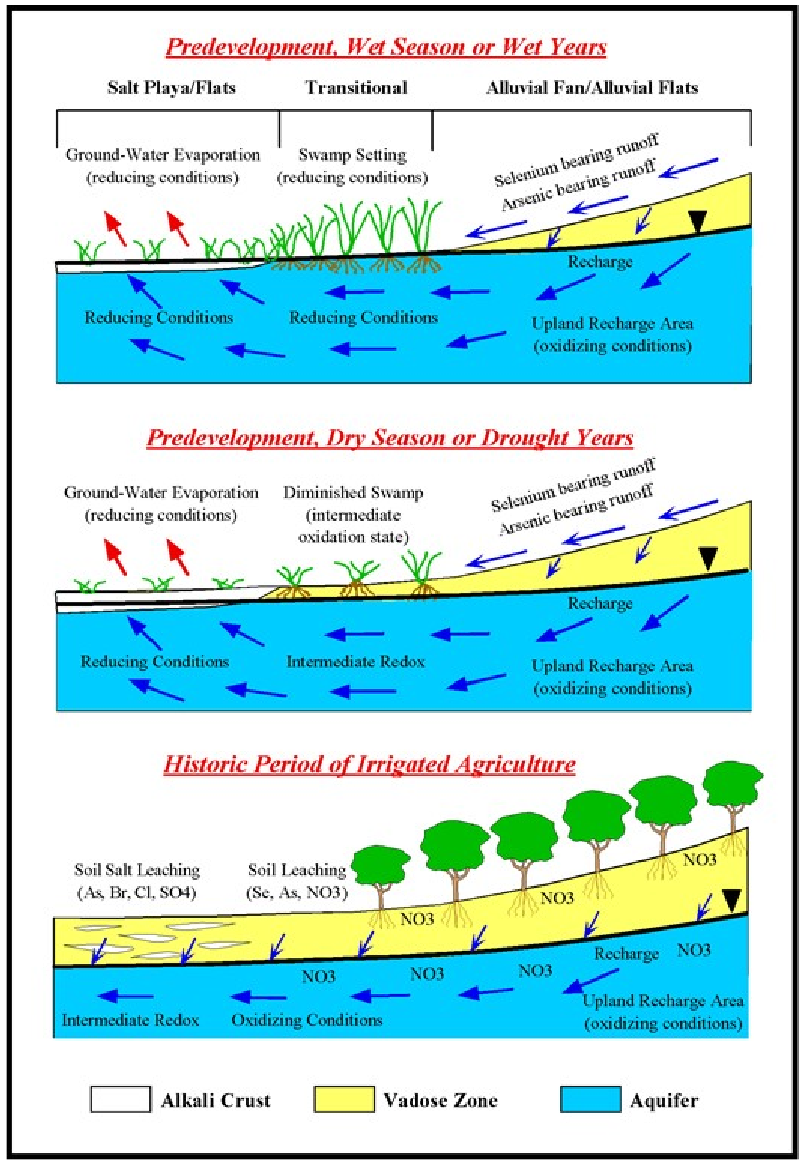
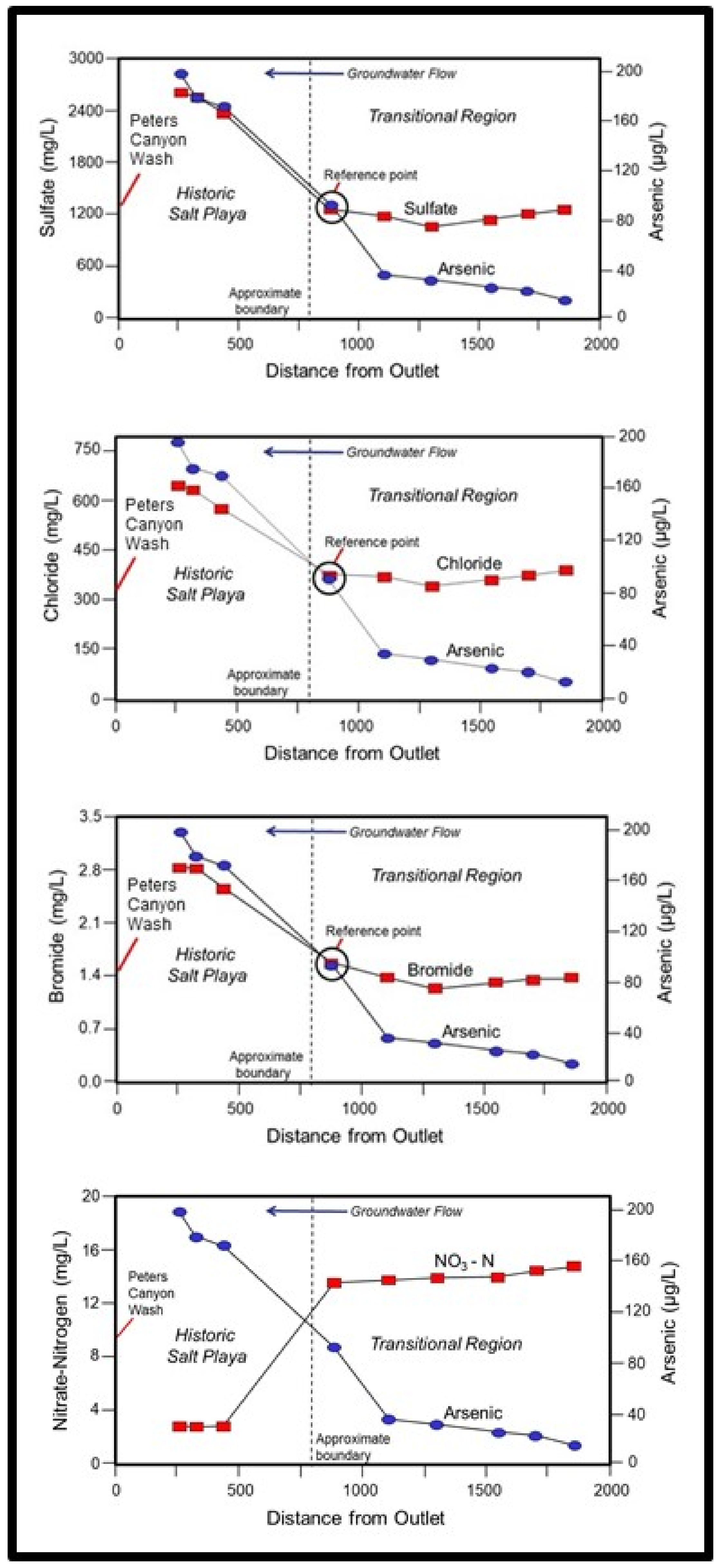
3.3. Flow Capacity and Toxic Trace Elements
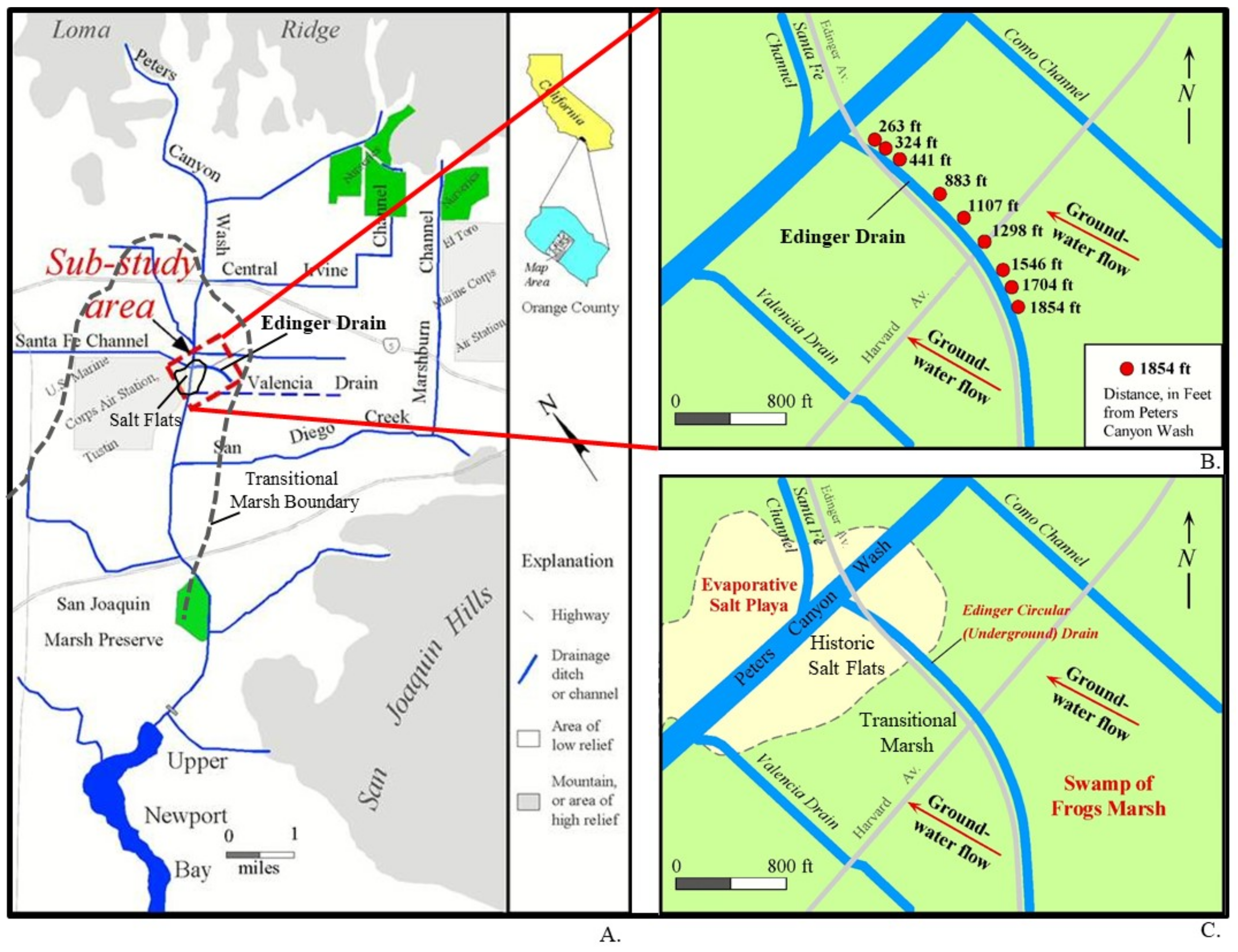
Case Example 3—Arsenic Loading to Groundwater from a Drained Phreatic Playa—San Diego Creek Watershed, USA
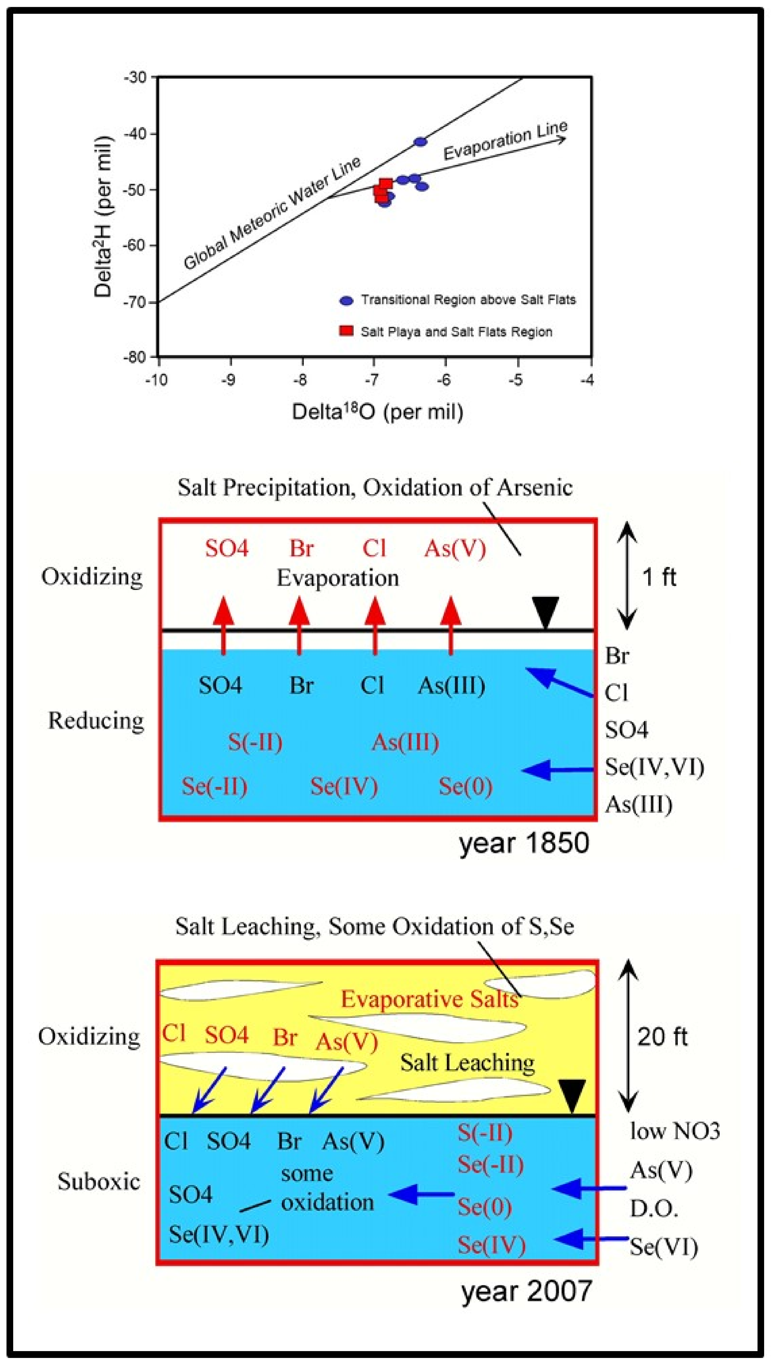
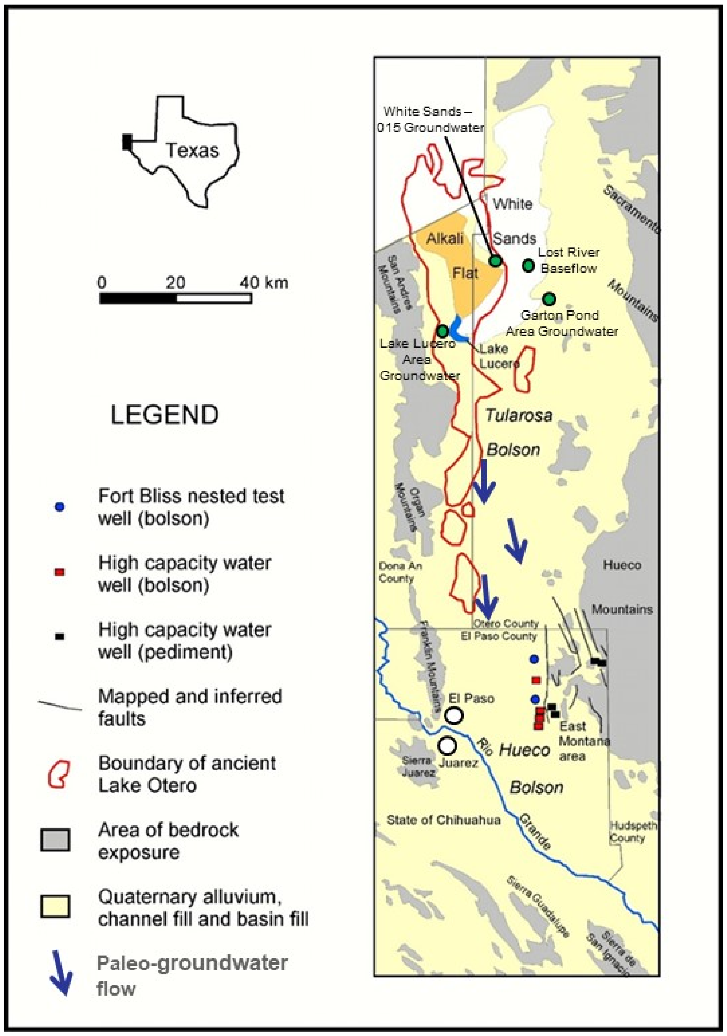
3.4. Isotope Hydrology and Flow Capacity
Case Example 4—Isotopically Evaporated Water in Eastern Hueco Bolson, USA
3.5. Flow Capacity, Fossil Hydraulic Gradients, and Groundwater Modeling
3.6. Fossil Hydraulic Gradients and Modeling Protocol
Case Example 5—Variable Density Modeling of Groundwater near a Phreatic Playa
4. Conclusions
Funding
Institutional Review Board Statement
Informed Consent Statement
Data Availability Statement
Acknowledgments
Conflicts of Interest
References
- Mifflin, M. Delineation of Groundwater Flow Systems in Nevada; Technical Report Series H-W, Hydrology and Water Resources Publication; University of Nevada-Reno, Desert Research Institute: Reno, NV, USA, 1968; Volume 4, p. 109. [Google Scholar]
- Hibbs, B.J.; Boghici, R.N.; Hayes, M.E.; Ashworth, J.B.; Hanson, A.T.; Samani, Z.A.; Kennedy, J.F.; Creel, B.J. Transboundary Aquifers of the El Paso/Ciudad Juarez/Las Cruces Region: Texas Water Development Board and New Mexico Water Resources Research Institute; Technical Contract Report; U.S. Environmental Protection Agency: Austin, TX, USA, 1997; p. 148.
- Hibbs, B. Long term climate change and environmental implications of aquifer flow capacity in arid groundwater basins. In Groundwater Sustainability, Hydro-Climate/Climate Change, and Environmental Engineering; Ahmad, S., Murray, R., Eds.; American Society of Civil Engineers: Reston, VA, USA, 2020; pp. 89–96. [Google Scholar]
- Anderson, T.W.; Welder, G.E.; Lesser, G.; Trujillo, A. Region 7, Central Alluvial Basins. In Hydrogeology—The Geology of North America; Back, W., Rosenshein, J.S., Seaber, P.R., Eds.; Geological Society of America: Boulder, CO, USA, 1988; Volume O-2, pp. 81–86. [Google Scholar]
- Gat, J.R. The relationship between surface and subsurface waters, water quality aspects in areas of low precipitation. Hydrol. Sci. J. 1980, 25, 257–267. [Google Scholar] [CrossRef] [Green Version]
- Sigstedt, S.; Phillips, F.; Ritchie, A. Groundwater flow in an ‘underfit’ carbonate aquifer in a semiarid climate: Application of environmental tracers to the Salt Basin, New Mexico (USA). Hydrogeol. J. 2016, 24, 841–863. [Google Scholar] [CrossRef]
- Haynes, C.V., Jr. Quaternary geology of the Tule Springs area, Clark County, Nevada. In Pleistocene Studies in Southern Nevada; Wormington, H.M., Ellis, D., Eds.; Nevada State Museum of Anthropology: Carson City, NV, USA, 1967; pp. 1–104. [Google Scholar]
- Mifflin, M.D.; Wheat, M.M. Pluvial lakes and estimated pluvial climates of Nevada. Nev. Bur. Mines Geol. Bull. 1979, 94, 57. [Google Scholar]
- Quade, J. Late Quaternary environmental changes in the upper Las Vegas Valley, Nevada. Quat. Res. 1986, 26, 340–357. [Google Scholar] [CrossRef]
- Hay, R.L.; Pexton, R.E.; Teague, T.T.; Kyser, T.K. Spring-related carbonate rocks, Mg clays and associated minerals in Pliocene deposits of the Amargosa Desert, Nevada and California. GSA Bull. 1986, 97, 1488–1503. [Google Scholar] [CrossRef]
- Quade, J.; Pratt, W.L. Late Wisconsin groundwater discharge environments of the Southwestern Indian Springs Valley, southern Nevada. Quat. Res. 1989, 31, 351–370. [Google Scholar] [CrossRef]
- Quade, J.; Mifflin, M.D.; Pratt, W.L.; McCoy, W.D.; Burckle, L. Fossil spring deposits in the southern Great Basin and their implications for changes in water-table levels near Yucca Mountain, Nevada, during Quaternary time. Geol. Soc. Am. Bull. 1995, 107, 213–230. [Google Scholar] [CrossRef]
- Miner, R.; Nelson, S.; Tingey, D.; Murrell, M. Using fossil spring deposits in the Death Valley region, USA to evaluate paleo flowpaths. J. Quat. Sci. 2007, 22, 373–386. [Google Scholar] [CrossRef]
- Matsubara, Y.; Howard, A.D. A spatially explicit model of runoff, evaporation, and lake extent; application to modern and late Pleistocene lakes in the Great Basin region, Western United States. Water Resour. Res. 2009, 45, W06425. [Google Scholar] [CrossRef]
- Pigati, J.S.; Miller, D.M.; Bright, J.; Mahan, S.A.; Nekola, J.C.; Paces, J.B. Chronology, sedimentology, and microfauna of ground-water discharge deposits in the central Mojave Desert, Valley Wells, California. Geol. Soc. Am. Bull. 2011, 123, 2224–2239. [Google Scholar] [CrossRef]
- Maxey, G. Hydrogeology of desert basins. Ground Water J. 1968, 6, 10–22. [Google Scholar] [CrossRef]
- Mifflin, M. Region 5, Great Basin. In Hydrogeology—The Geology of North America; Back, W., Rosenshein, J.S., Seaber, P.R., Eds.; Geological Society of America: Boulder, CO, USA, 1988; Volume O-2, pp. 69–78. [Google Scholar]
- Winograd, I.; Thordarson, W. Hydrogeologic and Hydrogeochemical Framework, South-Central Great Basin, Nevada-California, with Special Reference to the Nevada Test Sites; U.S. Geological Survey Professional Paper 712-C; U.S. Geological Survey: Reston, VA, USA, 1975; p. 126. [Google Scholar]
- Eakin, T.; Price, D.; Harrill, J.R. Summary Appraisals of the Nation’s Ground-Water Resources—Great Basin Region; U.S. Geological Survey Professional Paper 813-G; U.S. Geological Survey: Reston, VA, USA, 1976; p. 37. [Google Scholar]
- Hibbs, B.; Darling, B. Revisiting a classification scheme for USA-Mexico alluvial basin-fill aquifers. Ground Water J. 2005, 43, 750–763. [Google Scholar] [CrossRef]
- Hawley, J.; Kennedy, J.; Granados-Olivas, A.; Ortiz, M. Hydrogeologic Framework of the Binational Western Hueco Bolson-Paso del Norte Area, Texas, New Mexico, and Chihuahua; Technical Completion Report 349; New Mexico Water Resources Research Institute: Las Cruces, NM, USA, 2009. [Google Scholar]
- Boyd, F.; Kreitler, C. Hydrogeology of a Gypsum Playa, Northern Salt Basin, Texas; Report of Investigations No. 158; The University of Texas at Austin, Bureau of Economic Geology: Austin, TX, USA, 1986; p. 37. [Google Scholar]
- Stephens, D.B. Vadose Zone Hydrology; Lewis Publishers: Boca Raton, FL, USA, 1996; 347p. [Google Scholar]
- Newton, B.T.; Allen, B. Hydrologic Investigation at White Sands National Monument; Open-File Report; New Mexico Bureau Geology Mineral Resources: Socorro, NM, USA, 2014; Volume 0559, pp. 1–51. [Google Scholar]
- Waring, G.A. Ground Water in Pahrump, Mesquite, and Ivanpah Valleys Nevada and California; USGS Water Supply Paper, 450-C; USGS: Washington, DC, USA, 1920; pp. 51–85.
- Sims, D.B.; Spaulding, W.G. Shallow subsurface evidence for postglacial Holocene lakes at Ivanpah Dry Lake: An alternative energy development site in the Central Mojave Desert, California, USA. J. Geogr. Geol. 2017, 9, 1–24. [Google Scholar] [CrossRef] [Green Version]
- Duffy, C.; Al-Hassan, S. Groundwater circulation in a closed desert basin, topographic scaling and climatic forcing. Water Resour. Res. 1988, 24, 1675–1688. [Google Scholar]
- Hamann, E.; Post, V.; Kohfahl, C.; Prommer, H.; Simmons, C. Numerical investigation of coupled density-driven flow and hydrogeochemical processes below playas. Water Resour. Res. 2015, 51, 9338–9352. [Google Scholar] [CrossRef]
- Gehre, M.; Hoefling, R.; Lowski, P.; Strauch, G. Sample preparation device for quantitative hydrogen isotope analysis using chromium metal. Anal. Chem. 1996, 68, 4414–4417. [Google Scholar] [CrossRef]
- Craig, H. Isotopic variations in meteoric waters. Science 1961, 133, 1702–1703. [Google Scholar] [CrossRef]
- Craig, H. Standard for reporting concentrations of deuterium and oxygen-18 in natural waters. Science 1961, 133, 1833–1834. [Google Scholar] [CrossRef]
- Gonfiantini, R. Standards for stable isotope measurements in natural compounds. Nature 1978, 271, 534–536. [Google Scholar] [CrossRef]
- Pfaff, J.D. Method 300.0, Determination of Inorganic Anions by Ion Chromatography; Revision 2.1; United States Environmental Protection Agency: Washington, DC, USA, 1993.
- Hibbs, B.; Merino, M.; Andrus, R. Sources and Distribution of Selenium and Arsenic in Shallow Groundwater, San Diego Creek Watershed. In Selenium, Nitrate, and Other Constituents in San Diego Creek and Newport Bay Watersheds, 2004—2008; Technical Contract Report Prepared for the Santa Ana Regional Water Quality Control Board; California State University: Los Angeles, CA, USA, 2008. [Google Scholar]
- Hibbs, B.; Ortiz, M. New conceptual models of groundwater flow and salinity in the eastern Hueco Bolson aquifer. In Hydrological Resources in Transboundary Basins between Mexico and the United States; Granados, A., Ed.; University of Ciudad Press: Ciudad Juarez, Mexico, in press.
- Bedinger, M.S.; Sargent, K.A.; Langer, W.H. (Eds.) Studies of Geology and Hydrology in the Basin and Range Province, Southwestern United States, for Isolation of High-Level Radioactive Waste—Characterization of the Trans-Pecos region, Texas; U.S. Geological Survey Professional Paper 1370-B; U.S. Geological Survey: Reston, VA, USA, 1989; p. 43. [Google Scholar]
- Bedinger, M.S.; Sargent, K.A.; Langer, W.H. (Eds.) Studies of Geology and Hydrology in the Basin and Range Province, Southwestern United States, for Isolation of High-Level Radioactive Waste—Characterization of the Rio Grande Region, New Mexico and Texas; U.S. Geological Survey Professional Paper 1370-C; U.S. Geological Survey: Reston, VA, USA, 1989; p. 42. [Google Scholar]
- Montazer, P.; Wilson, W. Conceptual Hydrologic Model of Flow in the Unsaturated Zone, Yucca Mountain, Nevada; USGS Water-Resources Investigations Report 84-4345; U.S. Geological Survey: Reston, VA, USA, 1984. [Google Scholar]
- Montazer, P. Monitoring hydrologic conditions in the vadose zone in fractured rocks, Yucca Mountain, Nevada. In Flow and Transport through Unsaturated Fractured Rock; Geophysical Monograph; Evans, D.D., Nicholson, T.J., Eds.; American Geophysical Union: Washington, DC, USA, 1987; Volume 42. [Google Scholar]
- Nativ, R.; Adar, E.; Dahan, O.; Geyh, M. Water recharge and solute transport through the vadose zone of fractured chalk under desert conditions. Water Resour. Res. 1995, 31, 253–261. [Google Scholar] [CrossRef]
- Yang, I.; Rattray, G.; Yu, P. Interpretation of Chemical and Isotopic Data from Boreholes in the Unsaturated-Zone at Yucca Mountain, Nevada; 96-4058; U.S. Geological Survey: Reston, VA, USA, 1996. [Google Scholar]
- Scanlon, B.; Langford, R.; Goldsmith, R. Relationship between geomorphic settings and unsaturated flow in an arid setting. Water Resour. Res. 1999, 35, 983–999. [Google Scholar] [CrossRef]
- Scanlon, B.; Keese, K.; Flint, A.; Flint, L.; Gaye, C.; Edmunds, W.; Simmers, I. Global synthesis of groundwater recharge in semiarid and arid regions. Hydrol. Processes 2006, 20, 3335–3370. [Google Scholar] [CrossRef]
- Flint, A.; Flint, L.; Bodvarsson, G.; Kwickless, E.; Fabryka-Martin, J. Evolution of the conceptual model of the unsaturated zone hydrology at Yucca Mountain. J. Hydrol. 2001, 247, 1–30. [Google Scholar] [CrossRef]
- Stuckless, J.; Levich, R. Characterizing the proposed geologic repository for high-level radioactive waste at Yucca Mt. Nevada-Hydrology and Geochemistry. In Hydrology and Geochemistry of Yucca Mountain and Vicinity, Southern Nevada and California; Stuckless, J.S., Ed.; Geological Society of America: Boulder, CO, USA, 2012; p. 393. [Google Scholar]
- Stofhoff, S.; Walter, G. Average infiltration at Yucca Mountain over the next million years. Water Resour. Res. 2013, 49, 7528–7545. [Google Scholar] [CrossRef]
- Sheng, Z.; Devere, J. Systematic management for a stressed transboundary aquifer, the Hueco Bolson in the Paso del Norte region. J. Hydrogeol. 2005, 13, 813–825. [Google Scholar] [CrossRef]
- Hutchison, W. Groundwater Management in El Paso, Texas. Ph.D. Dissertation, The University of Texas, El Paso, TX, USA, 2006. [Google Scholar]
- Sneed, M.; Brandt, J.; Solt, M. Land Subsidence along the Delta–Mendota Canal in the Northern Part of the San Joaquin Valley, California, 2003–10; U.S. Geological Survey Scientific Investigations Report 2013–5142; U.S. Geological Survey: Reston, VA, USA, 2013; p. 87. [Google Scholar]
- Upper Los Angeles River Area Watermaster. Watermaster Service in the Upper Los Angeles River Area, Los Angeles County, 2012–2013; Watermaster Report for Water Year; Watermaster Service: Los Angeles, CA, USA, 2014. [Google Scholar]
- McGuire, V.L. Water-Level and Recoverable Water in Storage Changes, High Plains Aquifer, Predevelopment to 2015 and 2013–15; U.S. Geological Survey Scientific Investigations Report 2017–5040; U.S. Geological Survey: Reston, VA, USA, 2017; p. 14. [Google Scholar]
- James, M.; Montgomery, Inc. Remedial Investigation of Groundwater Contamination in San Fernando Valley, Remedial Investigation Report; Contract Report; City of Los Angeles Department of Water and Power: Los Angeles, CA, USA, 1992. [Google Scholar]
- Tetra Tech. Final Report, a Study on Seepage and Subsurface Inflows to Salton Sea and Adjacent Wetlands; Contract Report; Salton Sea Authority: La Quinta, CA, USA, 1999. [Google Scholar]
- Hibbs, B.; Sharp, J. Hydrogeological impacts of urbanization. Environ. Eng. Geosci. J. 2012, 18, 51–64. [Google Scholar] [CrossRef] [Green Version]
- Darling, B.K. Delineation of the ground-water flow systems of the Eagle Flat and Red Light Basins of Trans-Pecos Texas. Ph.D. Dissertation, The University of Texas at Austin, Austin, TX, USA, 1997; p. 179. [Google Scholar]
- Rosen, M.R.; Warren, J.K. The origin of groundwater-seepage gypsum from Bristol Dry Lake, California, U.S.A. Sedimentology 1990, 37, 983–996. [Google Scholar] [CrossRef]
- Rosen, M. Sedimentologic and geochemical constraints on the hydrologic evolution of Bristol Dry Lake, California, U.S.A. Paleogeography Palaeoclimatol. Paleoecol. 1991, 84, 229–257. [Google Scholar] [CrossRef]
- Rosen, M. The importance of groundwater in playas, a review of playa classifications and the sedimentology and hydrology of playas. Geol. Soc. Am. Spec. Publ. 1994, 289, 1–18. [Google Scholar]
- Hibbs, B.; Merino, M. A geologic source of salinity in the Rio Grande Aquifer. New Mex. J. Sci. 2006, 44, 165–181. [Google Scholar]
- Kreitler, C.W.; Mullican, W.F., III; Nativ, R. Hydrogeology of the Diablo Plateau, Trans-Pecos Texas. In Hydrogeology of Trans-Pecos Texas; Kreitler, C.W., Sharp, J.M., Jr., Eds.; The University of Texas at Austin Bureau of Economic Geology Guidebook: Austin, TX, USA, 1990; Volume 25, pp. 49–58. [Google Scholar]
- Izbicki, J.A.; Radyk, J.; Michel, R.L. Movement of water through the thick unsaturated zone underlying Oro Grande and Sheep Creek washes in the western Mojave Desert, USA. Hydrogeol. J. 2002, 10, 409–427. [Google Scholar] [CrossRef]
- Walvoord, M.A.; Scanlon, B.R. Hydrologic processes in deep vadose zones in interdrainage arid environments. In Groundwater Recharge in a Desert Environment: The Southwestern United States; Water Science and Applications Series; Hogan, J.F., Phillips, F.M., Scanlon, B.R., Eds.; American Geophysical Union: Washington, DC, USA, 2004; Volume 9, pp. 15–28. [Google Scholar]
- Dettinger, M.D. Reconnaissance estimates of natural recharge to desert basins in Nevada, U.S.A.; by using chloride balance calculations. J. Hydrol. 1989, 106, 55–78. [Google Scholar] [CrossRef]
- Hawley, J.W.; Hibbs, B.J.; Kennedy, J.F.; Creel, B.; Johnson, M.; Remmenga, M.; Lee, M.; Dinterman, P. Trans-International Boundary Aquifers in Southwestern New Mexico; Technical Contract Report Prepared for the U.S. Environmental Protection Agency; New Mexico Water Resources Research Institute: Las Cruces, NM, USA, 2000; p. 190. [Google Scholar]
- Anderholm, S.K. Mountain-Front Recharge Along the Eastern Side of the Middle Rio Grande Basin, Central New Mexico; U.S. Geological Survey Water-Resources Investigation Report 00-4010; U.S. Geological Survey: Reston, VA, USA, 2000. [Google Scholar]
- House, P.K.; Ramelli, A.R.; Buck, B.J. Surficial Geologic Map of the Ivanpah Valley Area, Clark County, Nevada; Map 156, Scale 1:50,000; Nevada Bureau of Mines and Geology: Reno, NV, USA, 2006. [Google Scholar]
- Malmberg, G.T. Hydrology of the Valley-Fill and Carbonate-Rock Reservoirs, Pahrump Valley, Nevada-California; U.S. Geological Survey Water-Supply Paper 1032; United States Government Publishing Office: Washington, SC, USA, 1967. [Google Scholar]
- ENSR Corporation. Final Report, Molycorp Supplemental Environmental Project Numerical Groundwater Flow Model Ivanpah Valley, San Bernardino County California and County, Nevada; Document No. 12044-001-300; California Regional Water Quality Control Board: Victorville, CA, USA, 2008. [Google Scholar]
- Glancy, P. Water-Resources Appraisal of Mesquite-Ivanpah Valley Area, Nevada and California; Reconnaissance Series Report 46; Nevada Department of Conservation and Natural Resources, Water Resources: Carson City, NV, USA, 1968; p. 57. [Google Scholar]
- Moyle, W. Water Wells and Springs in Ivanpah Valley, San Bernardino County, California; California Department of Water Resources Bulletin 91-21; Forgotten Books: London, UK, 1972; p. 56. [Google Scholar]
- TRC. New Ivanpah Evaporative Ponds RWCQB Cleanup and Abatement Order 6-98-20; Molycorp and California Regional Water Quality Control Board: Victorville, CA, USA, 2000. [Google Scholar]
- Antinao, J.L.; McDonald, E.V. An enhanced role for the Tropical Pacific on the humid Pleistocene-Holocene transition in southwestern North America. Quat. Sci. Rev. 2013, 78, 319–341. [Google Scholar] [CrossRef]
- Gill, T.E.; Gillette, D.A.; Niemeyer, T.; Winn, R.T. Elemental geochemistry of wind-erodible playa sediments, Owens Lake, California. Nucl. Instrum. Methods Phys. Res. Sect. B 2002, 189, 209–213. [Google Scholar] [CrossRef]
- Gao, S.; Fujii, R.; Chalmers, A.T.; Tanji, K.K. Evaluation of adsorbed arsenic and potential contribution to shallow groundwater in Tulare Lake bed area, Tulare Basin, California. Soil Sci. Soc. Am. J. 2004, 68, 89–95. [Google Scholar] [CrossRef]
- Gao, S.; Goldberg, S.R.; Chalmers, A.T.; Herbel, M.J.; Fujii, R.; Tanji, K.K. Sorption processes affecting arsenic solubility in Tulare lake bed sediments, California. Chem. Geol. 2006, 228, 33–43. [Google Scholar] [CrossRef]
- Kleinfelder. Screening Level Ecological Risk Assessment of Select Dust Control Measures Being Applied at Owens Lake, Keeler and Inyo County, California; Sapphos Environmental, Inc.: Pasadena, CA, USA, 2007; p. 44. [Google Scholar]
- ECORP Consulting, Inc. Tulare Lake Basin Hydrology and Hydrography, a Summary of the Movement of Water and Aquatic Species; U.S. Environmental Protection Agency: Austin, TX, USA, 2007; p. 87. [Google Scholar]
- US Bureau of Reclamation. A Summary of Hydrologic Data for the Test Case on Acreage Limitation in Tulare Lake, Sacramento, California; US Bureau of Reclamation: Sacramento, CA, USA, 1970. [Google Scholar]
- Summers Engineering. Tulare Lake Bed Coordinated Groundwater Management Plan. Prepared for Joint Powers Agreement. 2012, p. 26. Available online: http://kingsgroundwater.info/_documents/GWMPs/TLB-Coordinated-GWMP-lowres.pdf (accessed on 4 December 2021).
- Tulare Lake Basin Water Storage District. Proposed MUN Delisting Boundary Description; Tulare Lake Basin Water Storage District: Corcoran, CA, USA, 2012; p. 14. [Google Scholar]
- Swain, W.C.; Duell, L.F., Jr. Water Quality Data for Shallow Wells in the Western and Southern Tulare Basin, San Joaquin Valley, California, March to August, 1989; USGS Open-File Report 92-655; U.S. Geological Survey: Reston, VA, USA, 1993; p. 30. [Google Scholar]
- Fujii, R.; Swain, W.C. Areal Distribution of Selected Trace Elements, Salinity, and Major Ions in Shallow Ground Water, Tulare Basin, Southern San Joaquin Valley, California; U.S. Geological Survey Water-Resources Investigation Report 9504048; U.S. Geological Survey: Reston, VA, USA, 1995. [Google Scholar]
- Liebeck, J. Irvine—A History of Innovation and Growth; Malone, M., Ed.; Pioneer Publications: Houston, TX, USA, 1990; p. 156. [Google Scholar]
- Hibbs, B.; Lee, M. Sources of Selenium in the San Diego Creek Watershed, Orange County, California; Defend the Bay & California Urban Environmental Research and Education Center: Irvine, CA, USA, 2000. [Google Scholar]
- CRWQCB (California Regional Water Quality Control Board). Santa Ana Region. Draft Selenium (Se) Total Maximum Daily Load (TMDL); Newport Bay and San Diego Creek Watershed: Riverside, CA, USA, 2001. [Google Scholar]
- Meixner, T.; Hibbs, B.; Sjolin, J.; Walker, J. Sources of Selenium, Arsenic, and Nutrients in the Newport Bay Watershed; Contract Report Prepared for the Santa Ana Regional Water Quality Control Board. 2004. Available online: https://www.waterboards.ca.gov/rwqcb8/water_issues/programs/tmdl/docs/Meixner_etal_2004.pdf (accessed on 10 November 2021).
- Holmes, J.G. Soil survey around Santa Ana, Cal. In Field Operations of the Division of Soils; U.S. Department of Agriculture: Washington, DC, USA, 1901. [Google Scholar]
- Eckmann, E.C.; Strahorn, A.T.; Holmes, L.C.; Guernsey, J.E. Soil Survey of the Anaheim Area, California; U.S. Department of Agriculture, Advance Sheets-Field Operations of the Bureau of Soils; Nabu Press: Charleston, SC, USA, 1919; p. 79. [Google Scholar]
- Phillips, F.M.; Peeters, L.A.; Tansey, M.K.; Davis, S.N. Paleoclimatic inferences from an isotopic investigation of groundwater in the Central San Juan Basin, New Mexico. Quat. Res. 1986, 26, 179–193. [Google Scholar] [CrossRef]
- Dutton, A.R. Groundwater isotopic evidence for paleorecharge in US High Plains aquifers. Quat. Res. 1995, 43, 221–231. [Google Scholar] [CrossRef]
- Darling, B.K.; Hibbs, B.J.; Sharp, J.M. Integration of Carbon-14 and Oxygen-18 as a Basis for Differentiating Between Late Pleistocene and Post-Pleistocene Groundwater Ages Along Flow Paths of Two West Texas Bolson Aquifers; Geological Society of America Abstracts with Programs: Reston, VA, USA, 2017; Volume 49. [Google Scholar]
- Clark, I.; Fritz, P. Environmental Isotopes in Hydrogeology; CRC Press: New York, NY, USA, 1997; p. 328. [Google Scholar]
- Mazor, I.E. Chemical and Isotopic Groundwater Hydrology, the Applied Approach, 3rd ed.; Dekker, M., Ed.; CRC Press: Boca Raton, FL, USA, 2003; p. 472. [Google Scholar]
- Aggarwal, P.K. Isotope methods for dating old groundwater. In Isotope Methods for Dating Old Groundwater; Suckow, A., Aggarwal, P.K., Araguas-Araguas, L.J., Eds.; IAEA: Vienna, Austria, 2013; pp. 16–19. [Google Scholar]
- Deverel, S.; Thomas, J.; Decker, D.; Earman, S.; Mihevc, T.; Acheampong, S. Groundwater Evaporation Estimates Using Stable Isotope and Chloride Data, Yelland Playa, Spring Valley, Nevada; Publication No. 41219; Desert Research Institute: Las Vegas, NV, USA, 2005; p. 16. [Google Scholar]
- Dincer, T.; Al-Mugrin, A.; Zimmermann, U. Study of the infiltration and recharge through the sand dunes in arid zones with special reference to the stable isotopes and thermonuclear tritium. J. Hydrol. 1974, 23, 79–109. [Google Scholar] [CrossRef]
- US National Park Service. Geology of White Sands. Available online: https://www.nps.gov/whsa/learn/geology-of-white-sands.htm (accessed on 14 September 2021).
- Seager, W.R. Quaternary fault system in the Tularosa and Hueco Basins, southern New Mexico and West Texas. In New Mexico Geological Society, 31st Field Conference; New Mexico Geological Society: Socorro, NM, USA, 1980; pp. 131–135. [Google Scholar]
- Henry, C.D.; Gluck, J.K. A Preliminary Assessment of the Geologic Setting, Hydrology, and Geochemistry of the Hueco Tanks Geothermal Area, Texas and New Mexico; The University of Texas at Austin, Bureau of Economic Geology, Geological Circular 81-1: Austin, NV, USA, 1981; p. 48. [Google Scholar]
- Eastoe, C.; Hibbs, B.; Granados, A.; Hogan, J.; Hawley, J.; Hutchison, W. Isotopes in the Hueco Bolson aquifer, Texas (USA) and Chihuahua (Mexico)—Local and general implications for recharge sources in alluvial basins. Hydrogeol. J. 2009, 16, 737–747. [Google Scholar] [CrossRef]
- Bourdon, D.J. Flow of fossil groundwater. Q. J. Eng. Geol. Hydrogeol. 1977, 10, 97–124. [Google Scholar] [CrossRef]
- Lloyd, J.W.; Farag, M.H. Fossil ground-water gradients in arid regional sedimentary basins. Ground Water 1978, 16, 388–392. [Google Scholar] [CrossRef]
- Lloyd, J.; Miles, J. An examination of the mechanisms controlling groundwater gradients in hyper-arid regional sedimentary basins. J. Am. Water Resour. Assoc. 1986, 22, 471–478. [Google Scholar] [CrossRef]
- Heinl, M.; Brinkmann, P.J. A groundwater model of the Nubian aquifer system. Hydrol. Sci. J. 1989, 34, 425–447. [Google Scholar] [CrossRef] [Green Version]
- Schulz, S.; Walther, M.; Michelsen, N.; Rausch, R.; Dirks, H.; Al-Saud, M.; Merz, R.; Kolditz, O.; Schüth, C. Improving large-scale groundwater models by considering fossil gradients. Adv. Water Resour. 2017, 103, 32–43. [Google Scholar] [CrossRef]
- Bakiewicz, W.; Milne, D.; Noori, M. Hydrogeology of the Umm Er Radhuma aquifer, Saudi Arabia, with reference to fossil gradients. Q. J. Eng. Geol. Hydrogeol. 1982, 15, 105. [Google Scholar] [CrossRef]
- Howard, K.; Griffith, A. Can the impacts of climate change on groundwater resources be studied without the use of transient models? Hydrol. Sci. J. 2009, 54, 754–764. [Google Scholar] [CrossRef] [Green Version]
- Faulkner, R. Fossil water or renewable resource, The case for one Arabian aquifer: Proceedings of the Institution of Civil Engineers. Water Marit. Energy 1994, 106, 325–331. [Google Scholar]
- Tsur, Y.; Park, H.; Issar, A. Fossil groundwater resources as a basis for arid zone development? Int. J. Water Resour. Dev. 1989, 5, 191–201. [Google Scholar] [CrossRef]
- Ram, R.; Burg, A.; Zappala, J.; Yokochi, R.; Yechieli, Y.; Purtschert, R.; Jiang, W.; Lu, Z.; Mueller, P.; Bernier, R.; et al. Identifying recharge processes into a vast “fossil” aquifer based on dynamic groundwater 81Kr age evolution. J. Hydrol. 2020, 587, 124946. [Google Scholar] [CrossRef]
- De Vries, J.J.; Selaolo, E.T.; Beekman, H.E. Groundwater recharge in the Kalahari, with reference to paleo-hydrologic conditions. J. Hydrol. 2000, 238, 110–123. [Google Scholar] [CrossRef]
- Wulff, H.E. The Qanats of Iran. Sci. Am. 1968, 218, 94. [Google Scholar] [CrossRef]
- Garbrecht, G. Ancient Water Works—Lessons from History; Impact of Science on Society, UNESCO No.1; Science on Society: Paris, France, 1983; p. 10. [Google Scholar]
- English, P. Qanats and lifeworlds in Iranian plateau villages. In Transformation of Middle Eastern Natural Environment, Bulletin Series 103, Yale School of Forestry and Environmental Studies; Yale University: New Haven, CT, USA, 1997. [Google Scholar]
- Wilson, J.L.; Guan, H. Mountain-block hydrology and mountain-front recharge. In Groundwater Recharge in a Desert Environment: The Southwestern United States; Phillips, F., Hogan, J., Scanlon, B., Eds.; American Geophysical Union: Washington, DC, USA, 2004. [Google Scholar]
- Gleeson, T.; Manning, A.H. Regional groundwater flow in mountainous terrain: Three-dimensional simulations of topographic and hydrogeologic controls. Water Resour. Res. 2008, 44, W10403. [Google Scholar] [CrossRef]
- Gilbert, J.M.; Maxwell, R.M. Examining regional groundwater-surface water dynamics using an integrated hydrologic model of the San Joaquin River basin. Hydrol. Earth Syst. Sci. 2017, 21, 923–947. [Google Scholar] [CrossRef] [Green Version]
- Markovich, K.H.; Manning, A.H.; Condon, L.E.; McIntosh, J.C. Mountain-block recharge—A review of current understanding. Water Resour. Res. 2019, 55, 8278–8304. [Google Scholar] [CrossRef] [Green Version]
- Wright, E.P.; Benfield, A.C.; Edmunds, W.M.; Kitching, R. Hydrogeology of the Kufra and Sirte basins, eastern Libya. Q. J. Eng. Geol. Hydrogeol. 1982, 15, 83–103. [Google Scholar] [CrossRef] [Green Version]
- Houston, J.; Hart, D. Theoretical head decay in closed basin aquifers, an insight into fossil groundwater and recharge events in the Andes of northern Chile. Q. J. Eng. Geol. Hydrogeol. 2004, 37, 131–139. [Google Scholar] [CrossRef]
- Muller, T. Recharge and residence times in an arid area aquifer. Ph.D. Dissertation, Technical University of Dresden, Dresden, Germany, 2012; p. 157. [Google Scholar]
- Simmons, C.; Fenstemaker, T.; Sharp, J. Variable-density groundwater flow and solute transport in heterogeneous porous media: Approaches, resolutions and future challenges. J. Contam. Hydrol. 2001, 52, 245–275. [Google Scholar] [CrossRef]
- Brookings, D.G.; Thomson, B.M. Geochemical considerations for disposal facilities—Waste disposal in desert playas: In Deserts and Dumps? In The Disposal of Hazardous Materials in Desert Ecosystems; Reith, C.C., Thomson, B.M., Eds.; University of New Mexico Press: Albuquerque, NM, USA, 1992; p. 330. [Google Scholar]
- Whittemore, D.O. Geochemical differentiation of oil and gas brine from other saltwater sources contaminating water resources—Case studies from Kansas and Oklahoma. Environ. Geosci. 1995, 2, 15–31. [Google Scholar]
- Davis, S.N.; Whittemore, D.O.; Martin, J.F. Use of chloride/bromide ratios in studies of potable water. Groundwater 1998, 36, 338–350. [Google Scholar] [CrossRef]
- Cartwright, I.; Weaver, T.R.; Fifield, L.K. Cl/Br ratios and environmental isotopes as indicators of recharge variability and groundwater flows, an example from the southeast Murray Basin, Australia. Chem. Geol. 2006, 231, 38–56. [Google Scholar] [CrossRef]
- Freeman, J.T. The use of bromide and chloride mass ratios to differentiate salt-dissolution and formation brines in shallow groundwaters of the Western Canadian Sedimentary Basin. Hydrogeol. J. 2007, 15, 1377–1385. [Google Scholar] [CrossRef]


| Dug Wells at and above Ivanpah Playa—Sampled 1916 to 1917 | |||||||
|---|---|---|---|---|---|---|---|
| Well ID | Location | Chloride (mg/L) | Sulfate (mg/L) | Sodium + Potassium (mg/L) | TDS (mg/L) | Well Depth (m) | Depth to Water Table (m) |
| Old Borax Team Well | At Playa | 12,489 | 3921 | 8927 | 27,501 | 92 | 90 |
| S.E. Yates Well | At Playa | 3984 | 429 | 2416 | 7702 | 91 | 81 |
| Murphy Well | Above Playa | 30 | 51 | 55 | 335 | 116 | 92 |
| Soil Core Data, On and Off Playa Samples | |||||||||||||
|---|---|---|---|---|---|---|---|---|---|---|---|---|---|
| Core/ Parameter | 1 | 2 | 3 | Playa Edge | 4 | 5 | 6 | 7 | 8 | 9 | 10 | 11 | 12 |
| Location | At Playa | At Playa | At Playa | Above Playa | Above Playa | Above Playa | Above Playa | Above Playa | Above Playa | Above Playa | Above Playa | Above Playa | |
| Elevation (m) | 794.4 | 794.7 | 794.5 | 796.3 | 796.4 | 797.4 | 799.7 | 800.6 | 801.9 | 803.2 | 804.2 | 807.1 | |
| Chloride (mg/kg) | 53,061 | 121,664 | 162,911 | 2134 | 558 | 1572 | 725 | 689 | 391 | 211 | 637 | 1537 | |
| Sulfate (mg/kg) | 17,148 | 15,285 | 8212 | 7306 | 1592 | 2523 | 1072 | 1021 | 554 | 976 | 817 | 882 | |
| Sample ID | As(V) (µg/L) | As(III) (µg/L) | DMAs (µg/L) | MMAs (µg/L) | % as As (V) |
|---|---|---|---|---|---|
| Edinger Drain 1854 feet | 13.5 | <0.08 | <0.08 | <0.08 | ~100 |
| Edinger Drain 1704 feet | 20.8 | <0.08 | <0.08 | <0.08 | ~100 |
| Edinger Drain 1546 feet | 23.3 | <0.08 | <0.08 | <0.08 | ~100 |
| Edinger Drain 1298 feet | 29.2 * | -- | -- | -- | -- |
| Edinger Drain 1107 feet | 33.6 | <0.08 | <0.08 | <0.08 | ~100 |
| Edinger Drain 883 feet | 90.3 | <0.08 | <0.08 | <0.08 | ~100 |
| Transition Point | |||||
| Edinger Drain 441 feet | 170.0 | <0.08 | <0.08 | <0.08 | ~100 |
| Edinger Drain 324 feet | 176.0 | <0.08 | <0.08 | <0.08 | ~100 |
| Edinger Drain 263 feet | 196.0 | <0.08 | <0.08 | <0.08 | ~100 |
| Peters Canyon Wash—0 Feet | |||||
Publisher’s Note: MDPI stays neutral with regard to jurisdictional claims in published maps and institutional affiliations. |
© 2022 by the author. Licensee MDPI, Basel, Switzerland. This article is an open access article distributed under the terms and conditions of the Creative Commons Attribution (CC BY) license (https://creativecommons.org/licenses/by/4.0/).
Share and Cite
Hibbs, B.J. Commentary and Review of Modern Environmental Problems Linked to Historic Flow Capacity in Arid Groundwater Basins. Geosciences 2022, 12, 124. https://doi.org/10.3390/geosciences12030124
Hibbs BJ. Commentary and Review of Modern Environmental Problems Linked to Historic Flow Capacity in Arid Groundwater Basins. Geosciences. 2022; 12(3):124. https://doi.org/10.3390/geosciences12030124
Chicago/Turabian StyleHibbs, Barry J. 2022. "Commentary and Review of Modern Environmental Problems Linked to Historic Flow Capacity in Arid Groundwater Basins" Geosciences 12, no. 3: 124. https://doi.org/10.3390/geosciences12030124