CPT Data Interpretation Employing Different Machine Learning Techniques

Abstract

The classification of soils into categories with a similar range of properties is a fundamental geotechnical engineering procedure. At present, this classification is based on various types of cost- and time-intensive laboratory and/or in situ tests. These soil investigations are essential for each individual construction site and have to be performed prior to the design of a project. Since Machine Learning could play a key role in reducing the costs and time needed for a suitable site investigation program, the basic ability of Machine Learning models to classify soils from Cone Penetration Tests (CPT) is evaluated. To find an appropriate classification model, 24 different Machine Learning models, based on three different algorithms, are built and trained on a dataset consisting of 1339 CPT. The applied algorithms are a Support Vector Machine, an Artificial Neural Network and a Random Forest. As input features, different combinations of direct cone penetration test data (tip resistance q_c, sleeve friction f_s, friction ratio R_f, depth d), combined with “defined”, thus, not directly measured data (total vertical stresses σ_v, effective vertical stresses σ’_v and hydrostatic pore pressure u₀), are used. Standard soil classes based on grain size distributions and soil classes based on soil behavior types according to Robertson are applied as targets. The different models are compared with respect to their prediction performance and the required learning time. The best results for all targets were obtained with models using a Random Forest classifier. For the soil classes based on grain size distribution, an accuracy of about 75%, and for soil classes according to Robertson, an accuracy of about 97–99%, was reached.

1. Introduction

With the increasing number of available high-quality datasets, the application of machine learning algorithms has gained the interest of various fields of research over the last 10 years [1]. The classification of soils into groups with similar properties is a fundamental engineering task in the preliminary stages of a construction project. At this stage, the feasibility of the desired project is often not yet proved. Hence, monetary investments are associated with high risks. To keep the financial consequences of an unfeasible project low, (soil) investigation studies are usually cost-optimized. At present, investigation into subsoil using a combination of field and laboratory tests is inevitably associated with high costs; therefore, this process is often as minimal as possible. In recent years, the Cone Penetration Test (CPT) has gained interest as a powerful and cost-effective tool for the investigation of subsoil conditions. The goal of this paper is to utilize CPT data for the automatic interpretation of subsoil conditions.

Recent publications related to Cone Penetration Test data interpretation and soil classification using Artificial Intelligence show promising results. In these studies, Machine learning has been used to classify soils from CPT data [2,3,4,5] and to successfully estimate soil and design parameters [2,6]. Compared to these investigations, the basis of the present study is formed of a very large dataset of 1339 CPT tests, which were all performed in similar soils and conditions, with 490 of these tests are complemented by traditional soil classifications based on the European Soil Classification System (ESCS) [7,8]. Additionally, the ML models are used to predict soil classes from CPT tests conducted in the Netherlands, and thus outside the test area of the training data.

In this paper, a machine learning classifier based on a Support Vector Machine, Artificial Neural Network and Random Forest were used to predict soil classes according to Oberhollenzer et al. [8] and soil behavior types according to Robertson [9,10,11]. To identify the algorithm that is best suited to this task, 24 models were built and trained with varying sets of input features. The best results for each target, in terms of both prediction accuracy and training time, were obtained using the Random Forest classifier. The Random Forest models were also used to identify and predict soil strata from unseen CPT data from sites in Austria and the Netherlands, and led to very satisfying results.

It has to be noted that the application of machine learning does not automatically lead to cost-efficiency. However, regarding the interpretation of a high number of data or finding patterns in the obtained test data, machine learning could help to improve the interpretation quality and could reduce the time required for the classification. Thus, it may lead (in certain circumstances) to a reduction in costs.

2. Cone Penetration Test, Models and Methods

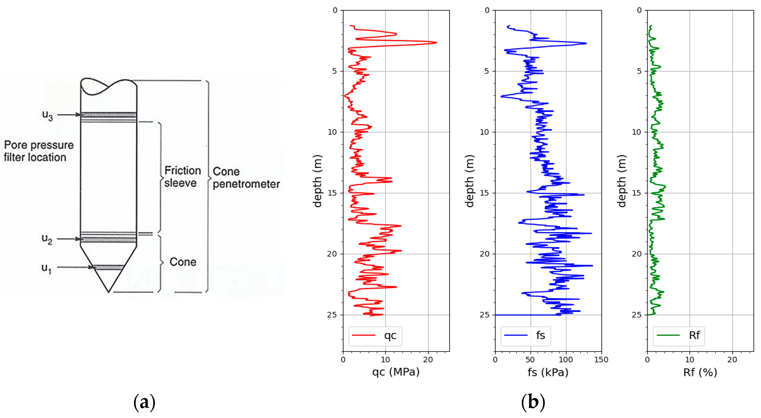
2.1. Cone Penetration Test (CPT)

In a CPT, a cone with a specific diameter gets pushed vertically into the ground under a constant rate. Based on the measured data, e.g., tip resistance q_c and sleeve friction f_s, various soil behavior charts were developed to identify the soil strata and soil behavior types [9,10,11,12,13]. Additionally, various empirical correlations have been published for a quick and easy interpretation of CPT data (including parameter determination). However, these correlations are generally not applicable to all soils and subsurface conditions and might need to be validated before their application (e.g., for over-consolidated soils [14,15] or reclaimed fills [16]). Figure 1a shows the scheme of the cone and Figure 1b shows a plot of the measured tip resistance q_c, sleeve friction f_s and the resulting friction ratio R_f (f_s/q_c in percent). In a piezocone test (CPTu), additional pore-pressures, due to groundwater (and installation effects) are measured (u₁, u₂, u₃). In a seismic cone penetration test (SCPT, SCPTu), the shear wave velocity Vs at specific penetration depth intervals (usually 50–100 cm) is measured. CPTs are mainly performed to determine subsoil conditions, such as soil type and strata, and to estimate geotechnical parameters (e.g., effective friction angle φ’, cohesion c, etc.) [17]. The disadvantages of a cone penetration test are that its application is limited to predominantly fine-grained soils and that the subsoil is not visible to the engineer. Therefore, the CPT tests are usually complemented by core drillings to verify the applicability of the correlations (e.g., for parameter identification).

2.2. Dataset

The dataset used for this study was published in 2021 by Graz University of Technology, in cooperation with the company Premstaller Geotechnik GmbH [8]. It is open-source and available for download under the following link: https://www.tugraz.at/en/institutes/ibg/research/computational-geotechnics-group/database/ (accessed on 1 October 2020).

The dataset consists of 1339 CPT tests from sites in Austria and southern Germany. All tests were performed by the company “Premstaller Geotechnik ZT GmbH”. For the tests, a CPT-truck or CPT-rig with a standardized 15 cm² probe was used.

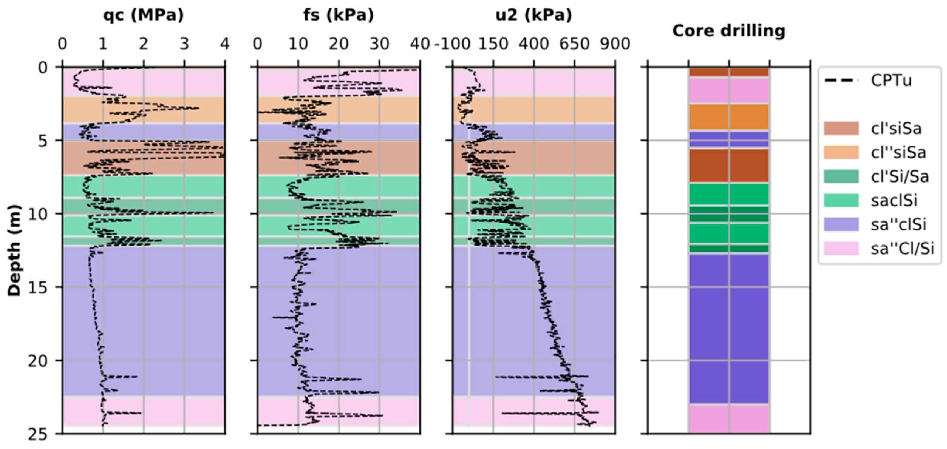
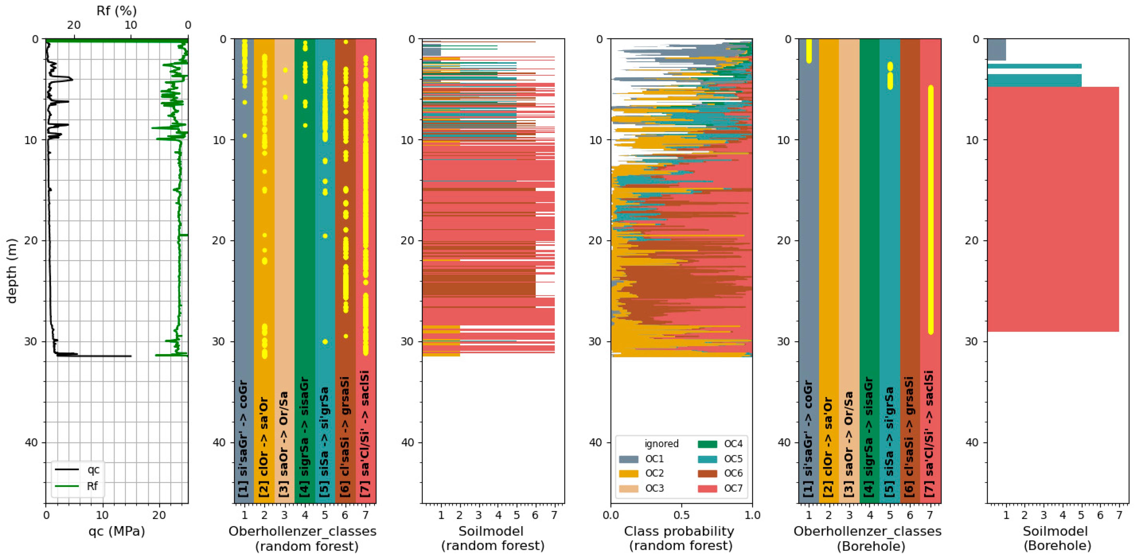
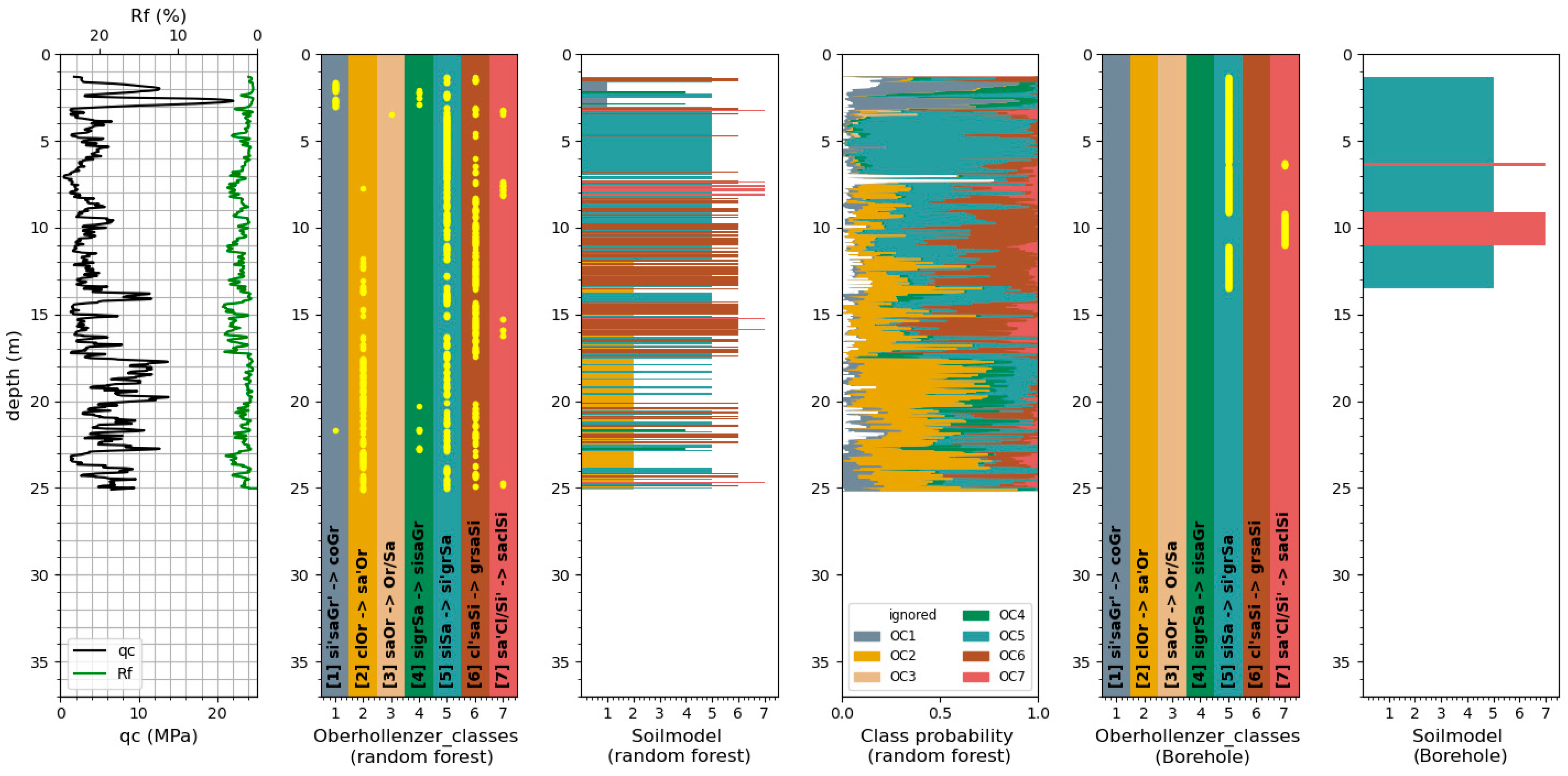
For the interpretation, the test data were processed with the software bundle CPeT-IT of Geologismiki to identify the soil behavior types according to Robertson [9,10,11]. Additionally, 490 of them were classified based on grain size distribution from adjacent boreholes. Figure 2 shows an example of the assignment of soil classification from borehole samples to the CPT data. The maximum distance between the CPT test and its adjacent borehole is approximately 50 m. Differences in the position of the soil layer changes, due to the distance between the CPT and borehole, were considered by manually adjusting the location of the soil layers by Oberhollenzer et al. [8].

The database contains 28 columns and 2,516,978 rows. The feature columns are distinguished in raw test data, data defined by an engineer and data based on empirical correlations (using the test and defined data). Measurement errors and outliers are eliminated by setting threshold values for the measured data of −100 and +10,000. Datapoints which exceed those boundaries are left blank.

The soil behavior types determined with the software package of Geologismiki [18] are based on the publications of Robertson from 2009, 2010 and 2016. In 1986, Robertson published the first chart for soil classification based on the cone penetration test data. With the cone resistance q_t (Pa), the friction ratio R_f (%) and the pore pressure ratio B_q (-), the chart distinguishes between 12 behavior types for predominantly fine-grained soils [13]. In 1990, Robertson provided a new soil behavior type classification based on normalized, and thus adapted to ground water conditions, CPT data. Additionally, the number of soil behavior types was decreased to nine [12]. An updated version of this chart using normalized parameters was published in 2009, where the normalized soil behavior types are determined by the soil behavior type index, I_c (-) (Equation (3)), which is calculated with the normalized cone resistance Q_t (-) and the normalized friction ratio F_r (-) [9]. In 2010, Robertson published an updated version of the soil behavior chart from 1986, where the 12 behavior types were adjusted to the nine types of 1990 [10]. Instead of q_t (Pa), this chart uses the dimensionless cone resistance q_c/p_a (-), where p_a (Pa) is the atmospheric pressure, and the friction ratio R_f (%), on both log scales. In 2016, Robertson published a new version of the soil behavior types, where the chart distinguishes between soil beyond the type, based on its behavior under loading. This is based on the updated normalized cone resistance Q_tn (-) (Equation (1)) and the normalized friction ratio F_r (%) (Equation (4)) [11]. The discussed soil behavior type charts are provided in Figure 3.

$$Q_{tn}=\left[\frac{\left(q_t-{\sigma }_v\right)}{p_a}\right]\ast {\left(\frac{p_a}{{\sigma }_v^{\prime }}\right)}^n$$

(1)

where n (-) is the stress exponent (Equation (2) and ≤1, which is based on the soil behavior type index I_c (-) (Equation (3)).

$$n=0.381\left(I_c\right)+0.05\left(\frac{{{\sigma }^{\prime }}_{vo}}{p_a}\right)-0.15$$

(2)

$$I_c=\sqrt{{\left(3.47-log{Q}_t\right)}^2+{\left(log{F}_r+1.22\right)}^2}$$

(3)

$$F_R=\frac{f_s}{q_t-{\sigma }_{vo}}\times 100\%$$

(4)

As mentioned above, an additional soil classification based on grain size distribution from adjacent boreholes was assigned to the 490 CPTs in the dataset by Oberhollenzer et al., in 2021 [8]. In this project, the borehole samples were classified according to ESCS [7]. Due to the fact that the soil classification of the borehole samples was performed by different engineers, the determined soil classes spread with regard to their denotation. Oberhollenzer et al. [8] summarized all classifications into seven different soil classes, henceforth called Oberhollenzer_classes (OC). These soil classes are summarized in

Table 1. Soil classification provided by Oberhollenzer et al. [8].

Name	Grain Size Range	Mainly Contents	Label
Group 1	Gr,sa,si’ → Gr,co	gravel	1
Group 2	Or,cl → Or,sa’	fine grained organic soils	2
Group 3	Or,sa → Or/Sa	coarse grained organic soils	3
Group 4	Sa,gr,si → Gr,sa,si	sand to gravel	4
Group 5	Sa,si → Sa,gr,si’	sand	5
Group 6	Si,sa,cl’ → Si,sa,gr	silt to fine sand	6
Group 7	Cl/Si,sa’ → Si,cl,sa	clay to silt	7
Ignored Group *	--	--	0

Gr = gravel; Sa = sand; Si = silt; Cl = clay; Or = organic soil; according to EN ISO 14688-1 [7]. * EN ISO 14688 classes which could not be assigned to OC Group 1–7.

. Classes which could not be assigned to one of the seven classes, e.g., due to the too widely spread classifications, are summarized in class 0 (ignored classifications).

2.2.1. Data Pre-Processing

In the pre-processing step, the dataset is evaluated with regard to its completeness and amount of data.

Since the number of samples is sufficiently high, rows with not a number (NAN) or null entries are deleted. For the learning models using grain-size-based soil classes as targets (Oberhollenzer_classes) 1,025,284 samples are available and, for the learning models using soil behavior types (SBT, SBTn, Mod. SBTn) as targets, 2,514,262 samples are available.

Table 2. Statistical information of the input features.

Target	Feature	Mean	Standard Deviation	Min	Max
Oberhollenzer_classes	Depth (m)	13.22	10.58	0.01	75.92
	qc (MPa)	5.34	8.41	−8.61	101.73
	fs (kPa)	54.76	70.40	−99.90	1591.40
	Rf (%)	2.49	38.16	−100.00	22,000.00
	σv (kPa)	251.12	200.94	0.19	1442.48
	u0 (kPa)	122.54	103.23	0.00	744.48
	σ’v (kPa)	128.58	99.69	0.09	697.70
Soil Behavior Types (SBT, SBTn, ModSBTn)	Depth (m)	12.40	10.43	0.01	103.00
	qc (MPa)	5.57	8.48	−8.61	122.90
	fs (kPa)	64.56	254.20	−100.00	47,436.00
	Rf (%)	2.70	43.32	−100.00	30,000.00
	σv (kPa)	235.68	198.21	0.19	1957.00
	u0 (kPa)	114.86	101.48	0.00	1010.43
	σ’v (kPa)	120.83	98.62	0.09	946.57

provides the mean, standard deviation, and numerical range of the input features.

For every target, two different sets of features are defined for training: one where only directly measured data, namely, q_c, f_s, R_f, and the depth are considered, and one where the total and effective vertical stresses σ_v and σ’_v, as well as the hydrostatic groundwater conditions u₀, are additionally considered. This leads to a total number of 24 models which are investigated in this study. Note: It was the intention of the authors to utilize as many data as possible to train the ML models, but only 362 CPTs were performed as CPTu. Therefore, it was decided to use q_c instead of q_t as an input feature.

The split of the data into subsets for training and validation and testing was done with the scikit-learn feature “train_test_split”, which randomly splits the samples into two datasets. The ratio of training and test data is defined as 80/20.

To ensure the uniform contribution of each feature to the training and prediction process, the features are scaled using the “StandardScaler” module. The features are scaled between −1 and +1 while the median is kept on the same level; therefore, the data are not biased by this process.

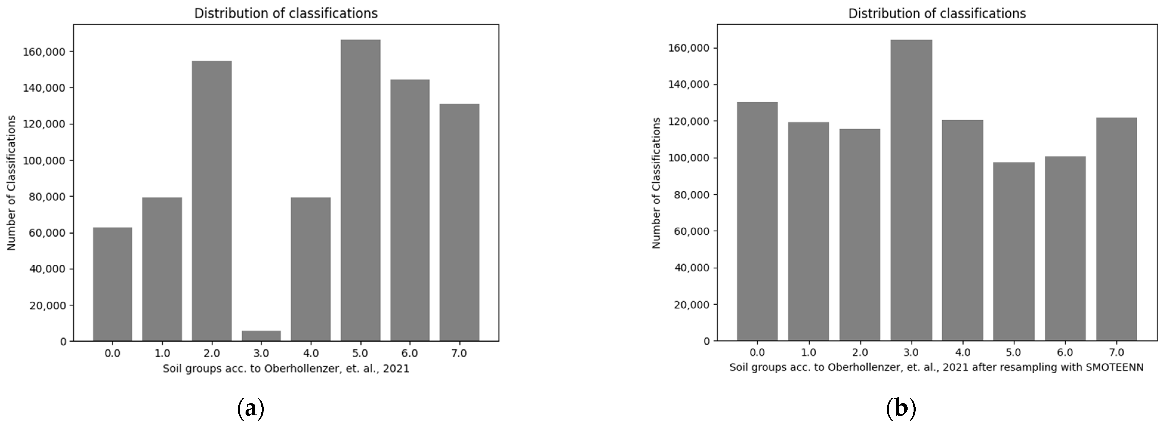
The uneven distribution of data between the classes could cause problems for the prediction performance of many machine learning algorithms. Unbalanced datasets can affect the learning model, e.g., if one class is highly underrepresented compared to the rest of the dataset, the model might ignore this class and still compute sufficient accuracy, but if the goal of the model is to find this specific class, then the model might be completely useless. In this study, the class balance of the data is considered within the Random forest models by setting the model parameter “class_weight” to ‘balanced’. This setting assigns a higher penalty to wrong classifications in minority classes. Another possible way to handle unbalanced data is the application of resampling algorithms. Two popular algorithms for this task are SMOTEENN and SMOTETomek. Both algorithms resample the data using a combination of under- and oversampling, which means that underrepresented classes are filled with synthetic data (which is based on the already available data), and data of overrepresented classes are removed, while statistical parameters like the mean and median of the data are kept on the same level. The difference between raw and resampled data is shown in Figure 4.

Preliminary studies showed that the application of these algorithms did not improve the overall model performance in this study and, additionally, the Random Forest models were barely susceptible to unbalanced data. Therefore, all models were trained with unbalanced datasets. More information on the sampling algorithms is provided on the imbalanced learning website [19].

2.3. Machine Learning Models—General Information

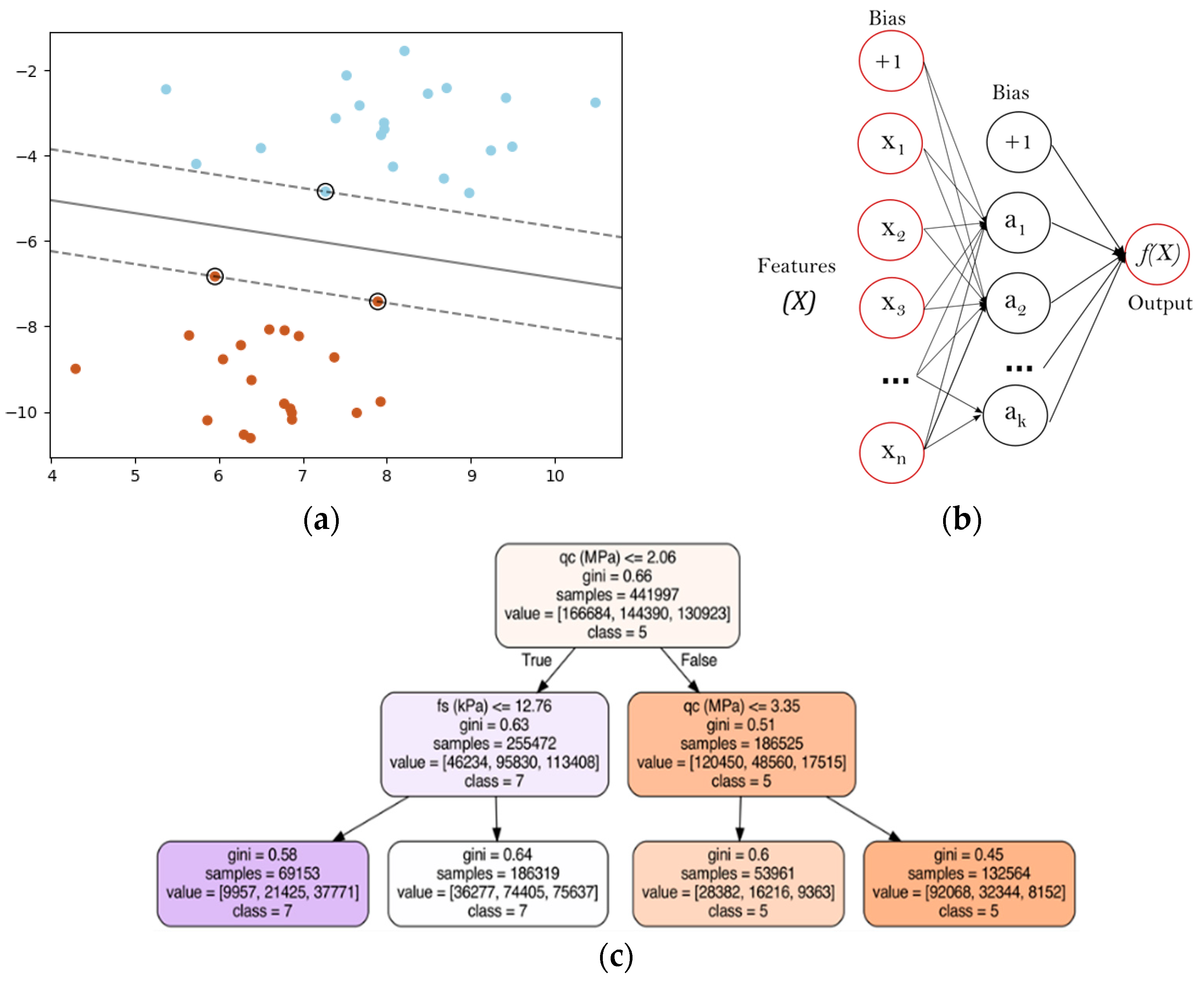
Machine learning (ML) has become a popular tool in various sciences for the interpretation of large datasets. The difference in the function principle of machine learning models compared to common computing algorithms is mainly that, rather than computing the results from an input and a predefined solution, the ML model finds a solution by learning from the input (features) with the respective output (targets), regardless of the specific algorithm (ANN, RF, etc.). The present study evaluates three different machine learning algorithms, namely, the Support Vector Machine, Artificial Neural Network and Random Forest. Their function principles are described briefly in the following section (Figure 5).

The Support Vector Machine (SVM) is a supervised learning algorithm for classification, regression, and detection of outliers [20]. For different tasks like classification and regression, the separating hyperplanes in a high or infinite dimensional space with the largest margin are to be found by the algorithm. The larger the margin, the lower the generalization error of the model. Figure 5a shows an example of a linear SVM. The samples on the boundaries are called support vectors. SVMs have recently been used in geotechnical engineering for soil classification [21], to estimate the bearing capacity of bored piles from CPT data [22] or for the assessment of soil compressibility [23].

The Artificial Neural Network is based on the function principle of a brain, and consists of three different types of layer (Figure 5b): first, the input layer, where the input features are handed to the model, second, the hidden layer(s), where the information of the input layers is combined with the weights, and third, the output layer, where the results are computed. The applied neural network in this study is a backpropagation algorithm, which is trained iteratively. Then, the output of the model is compared with the real targets of the training set to calculate the error and update the weights in the hidden layer(s). This process is performed until a minimum error is reached or the incremental improvement between iterations reaches zero. In recent research, ANNs have been used to classify soils from CPT data [3], identify soil parameters [24] or estimate the cone resistance of a cone penetration test [25].

The Random Forest (RF) is an ensemble of decision trees. A decision tree is a non-parametric supervised learning method that can summarize the decision rules from a series of data with features and labels, and use the structure of the tree to present these rules to solve classification and regression problems [26]. The solution of decision trees is comprehensible, and it is possible to identify the contribution of each input feature to the classification or regression model. Random forest models were recently used to predict the pile drivability [26], estimate geotechnical parameters [24] and, notably, the undrained shear strength [6]. Figure 5c shows an example of a decision tree with two splits for an ML model with two input features and three targets. The first line of the node provides the decision function; the second line provides the Gini impurity, which represents the probability of a random datapoint being classified as wrong and indicates the quality of a split (0.0 is best case; 1.0 is worst case). The third line indicates the number of samples which are observed in the node. The fourth line provides the final classification of the observed samples. The last line provides the most common resulting class, which was observed in the node [20].

The hyperparameter settings and input features of the applied machine learning models for this study are described in the following sections. All models are built on a MacBook Pro 13” 2018 (CPU: INTEL core i5 2.3 GHz quad core, RAM: 8 GB, GPU: Intel Iris Plus Graphics 655 1536 MB) using the SPYDER python environment. The Machine Learning algorithms used are part of the open-source-software library of scikit-learn [20].

2.3.1. Support Vector Machine

The evaluated Support Vector Classifier (SVC) uses a linear kernel function in order to keep training times low. A change in the kernel was investigated and showed that, for this interpretation, a radial basis function does not significantly improve the prediction accuracy but considerably increases the necessary learning time. The SVC models targeting soil classes based on grain size distribution (Oberhollenzer_classes) are evaluated without further hyperparameter modifications. The training and evaluation of SVC models targeting soil behavior types were cancelled due to the long necessary training time (compared to the other models), which exceeded 24 h. In contrast, the training times of ANN and RF models are within a few minutes.

Table 3. Proposed Models for each target and feature set.

Target	Model ID	Features
Oberhollenzer_classes	OC1_SVM, OC1_ANN, OC1_RF	Depth, qc, fs, Rf
	OC2_SVM, OC2_ANN, OC2_RF	Depth, qc, fs, σv, u0, σ’v, Rf
Soil Behavior Type (2010)	SBT1_SVM *, SBT1_ANN, SBT1_RF	Depth, qc, fs, Rf
	SBT2_SVM *, SBT2_ANN, STB2_RF	Depth, qc, fs, σv, u0, σ’v, Rf
Normalized Soil Behavior Type (2009)	SBTn1_SVM *, SBTn1_ANN, SBTn1_RF	Depth, qc, fs, Rf
	SBTn2_SVM *, SBTn2_ANN, SBTn2_RF	Depth, qc, fs, σv, u0, σ’v, Rf
Modified Normalized Soil Behavior Type (2016)	ModSBTn1_SVM *, ModSBTn1_ANN, ModSBTn1_RF	Depth, qc, fs, Rf
	ModSBTn2_SVM *, ModSBTn2_ANN, ModSBTn2_RF	Depth, qc, fs, σv, u0, σ’v, Rf

* These models were planned but not evaluated using SVM due to training times beyond 24 h.

shows the originally planned models for the support vector classifier. However, as stated above, only the two models for Oberhollenzer_classes are further analyzed and compared to the Artificial Neural Network and Random Forest models.

The influence of class balance on the model quality was considered by setting the hyperparameter “class_weight” to ‘balanced’. Then, the penalty size for wrong predictions is assigned with respect to the amount of data in each class. This leads to a higher penalty for wrong predictions in minority classes. The evaluation of the obtained results shows that, in the considered problem, the overall performance of the SVM models does not increase when considering the class balance with the hyperparameter “class_weight”. Sampling algorithms are not used for the SVM models.

2.3.2. Artificial Neural Network Models

The artificial neural network models are built using the MLPCLassifier module of the scikit-learn library. The network size is chosen based on recommendations provided by Heaton [27]. Similar to the support vector classifier, eight different models are analyzed. The best combination of hyperparameters is evaluated and determined using grid search techniques, where a range for each parameter is defined. The chosen hyperparameters are then validated using cross-validation. In order to keep the training times within acceptable limits, the number of hidden layers is set to a maximum of three and the number of neurons in these layers is set to a maximum of 10. (Note: It would be possible to increase the number of hidden layers and neurons, which would also slightly increase the prediction accuracy of the models. However, the training times would increase significantly, and thus would no longer be comparable to the training times of Random Forest models).

During the grid search analysis, a range of settings was tested for the number of hidden layers, the number of neurons, the activation function, the learning rate and the solver. For the activation function, learning rate and the solver modifications, aside from the default settings, do not significantly increase the model performance; therefore, the default parameters are used for model evaluation. The number of hidden layers and neurons are evaluated in individual steps. First, three sets with one, two and three layers of 10 neurons are evaluated. Then, three different sets of neurons in one layer are evaluated. The best combination was identified with three layers of 10 neurons for both targets, the soil classes based on grain size distribution and soil behavior types. Note: To obtain the best possible prediction accuracy for soil classes based on grain size distribution, the number of hidden layers and neurons must be increased further. This would result in a higher accuracy of about 8–10%. However, the resulting model accuracy is still much lower (10–15%) compared to the Random Forest models (see next chapter). Therefore, it was decided to keep the training times comparable in this study, within the range of from 10 to 30 min. The further optimization of the prediction with neural networks with deeper and more sophisticated networks is part of the ongoing research at the Institute of Soil Mechanics, Foundation Engineering and Numerical Geotechnics at Graz University of Technology.

2.3.3. Random Forest Models

The Random Forest classifier used in this study is part of the ensemble learning module of scikit-learn. Similar to the ANN models, the best set of hyperparameters is determined via cross-validation. Additionally, cross-validation is used to plot learning and validation curves to identify the bias and variance of the model. Cross-validation and hyperparameter tuning are performed for the models targeting Oberhollenzer_classes and soil behavior types. Since the properties of all soil behavior types are quite similar, they are only performed once for all models targeting soil behavior types (SBT, SBTn, ModSBTn). An overview of the models based on the random forest classifier is provided in Table 3.

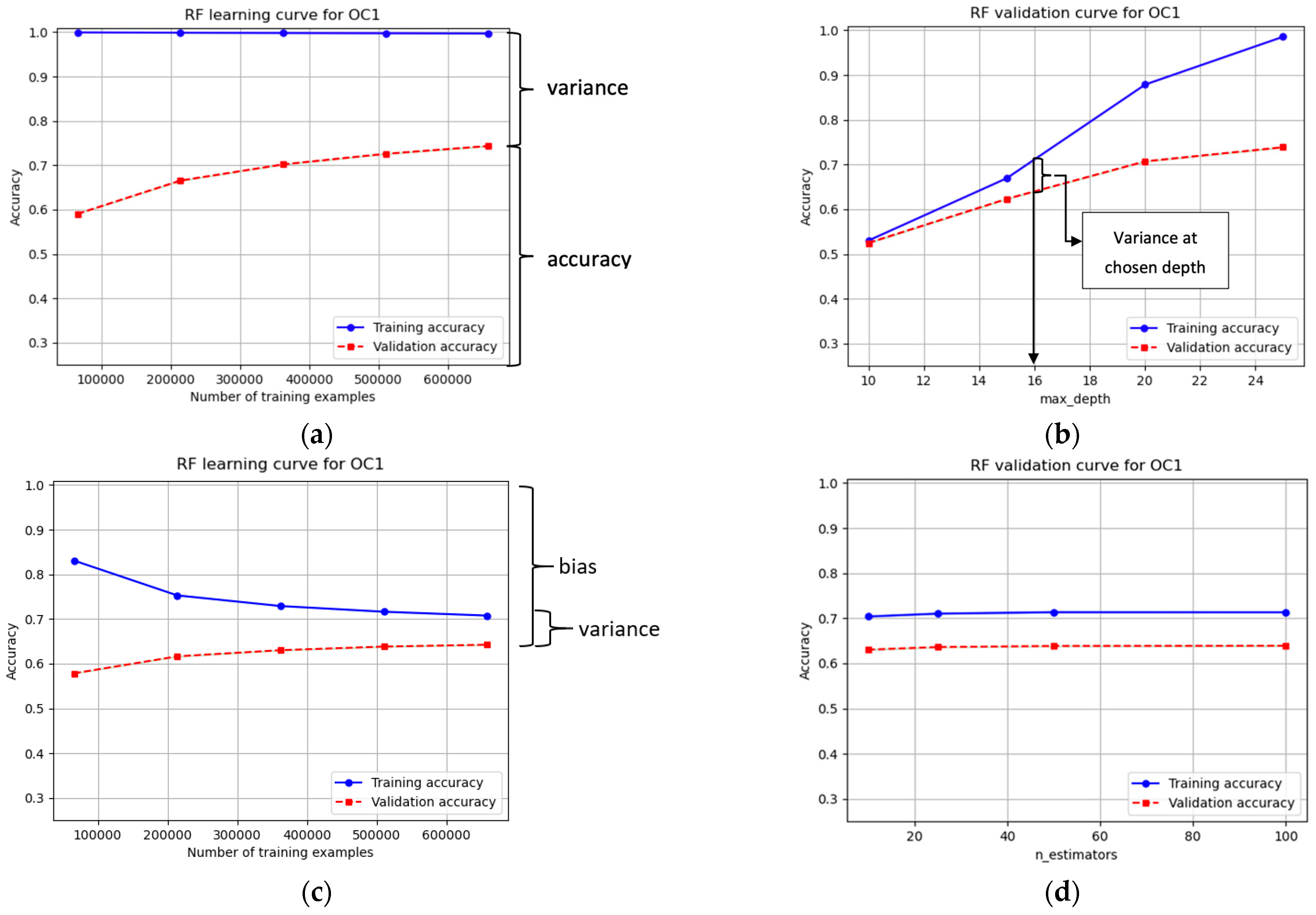
The RF models are analyzed using learning and validation curves to visualize bias and variance, which indicates susceptibility to over- or underfitting. In order to obtain a robust model, bias and variance should be kept low [28]. The difference between training and validation accuracy is referred to as variance. High variance causes a model that is not able to generalize very well, which results in a much higher training accuracy than validation accuracy. A high bias means that the data are too complex for the model. One of the main hyperparameters governing bias and variance of an RF model, is the maximum size of each tree (“max_depth”) in the forest. Figure 6 displays the process of hyperparameter optimization. In the learning curve without the limitation of tree-size (Figure 6a), the curves show high variance. By plotting the validation curve (Figure 6b), the influence of a specific hyperparameter, in this case the “max_depth” is visualized. After adjusting the settings for the respective hyperparameter (in this case, to 16), the learning curve is plotted again (Figure 6c), and a reduced variance of nearly 20% can be seen. By reducing the variance, the bias also increases (in this case, ~10%); therefore, a good trade-off must be found. Compared to the size of each tree, the number of trees (n_estimators) does not influence the bias and variance of the model, which is shown in Figure 6d.

2.4. Training, Validation and Testing

After pre-processing the data, the building process of a machine learning models can be divided into three different steps: First the training step, where the machine learning algorithm learns from the training data. This is an iterative process, which ends when a desired minimum error or maximum accuracy, or a predefined maximum number of iterations, is reached. Second, the validation step, where the model is analyzed regarding generalization properties such as overfitting and underfitting, whereas overfitting (high variance) means that the model fits better to the training data than to validation data and underfitting (high bias) means that the data are too complex for the chosen model. To eliminate errors due to the distribution of the data in the dataset, the validation is usually performed with cross-validation (CV) techniques [28]. The most common form of the CV is k-fold cross validation. Here, the training data are split k-times into sets for training and testing. As a result of the CV, learning and validation curves can be plotted. Third, the testing step where the model with the desired hyperparameter set is tested on unseen data from the test dataset (usually 20–30% of the entire data) [28]. A schema of the data used for the three aforementioned steps is given in

Table 4. Schema of utilized data in k-fold cross validation [20].

Schema of k-fold Cross Validation
	Entire Dataset
Split	Training Data				Test Data (not used for validation)
1st fold	Validate	Train			Not used for validation
2nd fold	Train	Validate	Train
3rd fold	Train		Validate	Train
4th fold	Train			Validate

. The results of the testing step are then used to generate the classification report and confusion matrix.

2.5. Model Comparison

The confusion matrix contains information about the distribution and uniformity of classification results through the target classes, and thus also indicates the influence of class balance on the model. Table 4 schematically shows the content of a confusion matrix, where true positive means that the model prediction is positive, and the actual state is positive. False negative means that the model prediction is negative, but the actual state is positive. False positive means that the model prediction is positive, but the actual state is negative and true negative means that the predicted and actual state are both negative. The classification report (

Table 5. Schema of a confusion matrix for the evaluation of results [20].

		Actual
		Positive	Negative
Predicted	Positive	True Positive (TP)	False Positive (FP)
	Negative	False Negative (FN)	True Negative (TN)

), however, contains the classification results in terms of accuracy (describes the percentage of the correct classifications), precision (defined as the positive correct predictions), recall (describes what percentage of positive cases the model catches) and the f1-score (weighted ratio between the precision and recall). All values are given as a percentage, where 100% is the best and 0% is the worst. In addition, the results of the classification report are provided as a weighted average (Equation (5)), which is the average score of all classes, weighted by the number of classifications.

$$weighted avg=\frac{{\displaystyle \sum }\left(score of each class\ast n_{classifications in class}\right)}{n_{all classifications}}$$

(5)

3. Results

3.1. Support Vector Machine

As mentioned in Section 2.2.1 for the support vector machine, the results are only obtained from models using Oberhollenzer_classes as targets. The database for soil behavior type models contains approximately twice as many data as the OC database. Therefore, the training times of the support vector classifier for SBT models are extremely high when compared to ANN and RF models. Regardless of the applied kernel function, the training times always exceed 25 h. On the contrary, the training times of ANN and RF models are consistently within a few minutes (depending on the simultaneously running processes of the hardware). Hence, it was decided to not evaluate these models any further. Additionally, since the training time of the OC_SVM models is approximately 12 h, which is far longer than ANN or RF (in combination with poor classification accuracy), the cross-validation step was skipped.

However, the results of the two analyzed models, OC1_SVM and OC2_SVM, are provided in Table 9. Although the training times of the SVM models are the longest by far, regardless of the kernel function, the obtained accuracies are the lowest. With an accuracy of about 38% and a training time of about 12 h, it can be assumed that the SVM is not sufficient for this dataset or, in other words, not well-suited to this type of application.

3.2. Artificial Neural Network

Classification models based on artificial neural network algorithms also lead to low prediction accuracies when used for Oberhollenzer_classes. However, the training times are similar to RF and within a few minutes. The obtained accuracies for OC models are 46% and 47% for OC1_ANN and OC2_ANN, respectively. To evaluate the influence of the number of hidden layers and neurons on the overall model quality, one training run is carried out, where these hyperparameters are set to three layers, with 100 neurons in each. The computed results showed that this leads to an increased accuracy (~55%); however, as a consequence of this hyperparameter adjustment, the training time increases to 12 h. Considering the highly increased training time, with only a small effect on the gained accuracy, it is assumed that the model with three hidden layers of 10 neurons (as described in Section 2.3.2) is a good trade-off for this study.

In contrast to the OC_ANN models, the models for soil behavior type classifications predict a very high accuracy, consistently above 94%. The models using additional information related to the vertical stresses and hydrostatic pore pressures (SBT2_ANN, SBTn2_ANN, ModSBTn2_ANN) give even better results, with accuracies consistently at about 98% (and beyond). Additionally, the training times are similar to the random forest models (a few minutes). The result of each ANN model is provided in Table 8.

3.3. Random Forest

The models based on a random forest algorithm lead to the highest prediction accuracies of all evaluated models. Models for the Oberhollenzer_classes predicted an accuracy of about 65% (OC1_RF) and 75% (OC2_RF). Additionally, the training times of the RF models are the lowest, being within a few minutes.

The prediction accuracy of random forest models for the soil behavior type classifications is nearly 100% (97–99%). The training times of these models are also slightly lower than the training times of ANN models. Another point which should be mentioned is that the RF models are the easiest to apply regarding hyperparameter settings.

Table 6. Confusion matrix for OC2_RF.

OC2_RF		Confusion Matrix
		Predicted
		0	1	2	3	4	5	6	7
Actual	0	10,789	1358	716	12	588	1322	588	421
	1	1084	13,968	505	19	1240	2236	609	281
	2	474	409	30,722	38	729	2630	2066	1403
	3	51	39	413	689	32	68	55	65
	4	870	2015	800	14	12,104	2908	534	297
	5	719	1304	1121	13	985	33,760	2805	1042
	6	800	581	1596	50	526	4713	26,080	1817
	7	509	285	993	43	220	1433	2579	26,722

Bold values are related to correct classifications.

,

Table 7. Confusion matrix for ModSBTn2_RF.

ModSBT n2_RF		Confusion Matrix
		Predicted
		0	1	2	3	4	5	6	7
Actual	0	18,243	114	69	0	142	78	122	139
	1	110	38,476	477	0	113	0	4	3
	2	17	367	120,717	286	154	13	0	1
	3	0	2	267	34,202	1	192	0	0
	4	15	113	220	0	30,499	89	238	14
	5	6	0	3	197	111	32,106	1	278
	6	35	2	0	0	245	2	64,811	480
	7	48	0	0	0	5	244	491	158,291

Bold values are related to correct classifications.

and

Table 8. Classification report for ModSBTn2_RF and OC2_RF.

Classification Report
Model	Score	Weighted Avg.
ModSBTn2_RF	Accuracy	0.99
	Precision	0.99
	Recall	0.99
	F1-score	0.99
OC2_RF	Accuracy	0.75
	Precision	0.76
	Recall	0.75
	F1-score	0.75

provide the confusion matrices of the models OC2_RF and ModSBTn2_RF, respectively. The corresponding classification reports are provided in Table 8. The confusion matrix provides the distribution of correct and incorrect classifications for the obtained test samples. The diagonal values (in bold) indicate the correct predictions, and the rest show the incorrect predictions for each class. A relatively uniform distribution of correct and incorrect classifications across all classes, combined with high accuracy, usually indicates a good generalization performance of the evaluated model. The classification report provides the scores described earlier in Section 2.4. From the confusion matrix and classification report of OC2_RF and ModSBTn2_RF, it could be concluded that RF models seem to be very efficient for the interpretation of CPT data.

3.4. Comparison

The best model performance through all classification targets and feature sets is obtained using a random forest algorithm, in terms of both accuracy and training time. The result of each model is provided in

Table 9. Results of all analyzed models.

Target	Model ID	Algorithm	Features	Accuracy
OC	OC1_SVM	SVM	Depth, qc, fs, Rf	0.38
	OC2_SVM	SVM	Depth, qc, fs, σv, u0, σ’v, Rf	0.38
	OC1_ANN	ANN	Depth, qc, fs, Rf	0.46
	OC2_ANN	ANN	Depth, qc, fs, σv, u0, σ’v, Rf	0.47
	OC1_RF	RF	Depth, qc, fs, Rf	0.65
	OC2_RF	RF	Depth, qc, fs, σv, u0, σ’v, Rf	0.75
SBT	SBT1_ANN	ANN	Depth, qc, fs, Rf	0.98
	SBT2_ANN	ANN	Depth, qc, fs, σv, u0, σ’v, Rf	0.98
	SBT1_RF	RF	Depth, qc, fs, Rf	0.99
	SBT2_RF	RF	Depth, qc, fs, σv, u0, σ’v, Rf	0.99
SBTn	SBTn1_ANN	ANN	Depth, qc, fs, Rf	0.95
	SBTn2_ANN	ANN	Depth, qc, fs, σv, u0, σ’v, Rf	0.97
	SBTn1_RF	RF	Depth, qc, fs, Rf	0.97
	SBTn2_RF	RF	Depth, qc, fs, σv, u0, σ’v, Rf	0.99
Mod.SBTn	MSBTn1_ANN	ANN	Depth, qc, fs, Rf	0.94
	MSBTn2_ANN	ANN	Depth, qc, fs, σv, u0, σ’v, Rf	0.98
	MSBTn1_RF	RF	Depth, qc, fs, Rf	0.97
	MSBTn2_RF	RF	Depth, qc, fs, σv, u0, σ’v, Rf	0.99

.

In summary, it can be concluded that the SVM models are not well-suited to this type of task and data. The ANN models perform very well for the determination of soil behavior types from the CPT data, but, in contrast, the prediction of soil classes based on grain-size distribution was not sufficient. The RF models resulted in the best classifications for each combination of input features and target classes analyzed. Furthermore, the positive influence of additional information on the stresses and groundwater conditions in the subsoil is recognizable in the improved model accuracies after adding the effective and total vertical stresses, σ’_v and σ_v, as well as the hydrostatic pore pressures, u₀, to the feature set.

4. Application—Classification of Unseen CPT Data

Since the random forest model yielded adequate results for soil classification, both in the prediction of soil classes based on grain size distribution and soil classes based on empirical correlations with the CPT data (SBT, SBTn, ModSBTn), the RF models are used in the next step to predict the soil classes of unseen CPT data from sites inside and outside Austria. In the following, the results of one CPT from Austria and one from a CPT performed in the Netherlands are discussed.

4.1. CPT Data from Austria

The results of soil classification using the random forest model are provided below. Figure 7 displays the CPT data (q_c, R_f) along with the predicted soil classes (OC) and the resulting soil model, as well as the probability of each class. Additionally, for comparison, the soil classes and the soil model determined from an adjacent borehole are presented. The class probability plot provides the probability of each class for every depth step, where the class with the highest probability is also the resulting soil class predicted by the ML model.

From 0 to 5 m below surface elevation, the model predicts mixtures of sand, gravel and silt (OC 1–5). From 5–10 m, mainly sand, silt and clay are identified (OC 5–7), whereas below 10 m, the model mainly classifies silt and clay (OC 6–7). (Note: Class 2 consists of fine-grained organic soils; therefore, the physical behavior under cone penetration seems to be quite similar to class 7. This could be a possible explanation for the classification of fine-grained organic soils in the last 4–5 m). The comparison of the predicted soil model with the soil model from the adjacent borehole shows that the RF model is able to identify the coarse-grained soils in the first 5 m of the test quite well. The range between 5 and 10 m deviates somewhat from the borehole classification, but the most-predicted classes refer to a mixture of sands, silts and clays, which is quite comprehensible in view of the CPT data. Additionally, the predicted classes below 10 m in depth are nearly similar to the borehole classification. The depth of the borehole is not equal to the penetration depth of the CPT; therefore, the last meters cannot be compared.

Besides the soil classification based on grain size distribution, classification based on soil behavior types is also evaluated. Figure 8 shows the CPT data, along with the predicted, modified, normalized soil behavior type (Mod.SBTn) of the RF model. Additionally, for comparison, the soil behavior type is determined using the software bundle of Geologismiki. As expected from the testing results of the model, the classification result is almost identical to the one determined based on empirical correlations using Geologismiki, since, compared to the Oberhollenzer_classes, soil behavior types are determined with empirical correlations from the CPT data. Consequently, the random forest models for soil behavior types predictwith a higher accuracy than those for Oberhollenzer_classes. Additionally, the plotted class probabilities are much more clearly distributed than those in the prediction of OCs and, thus, the classifications are more robust.

4.2. CPT Data from The Netherlands

The random forest models are additionally used to classify soils from CPT performed in the Netherlands, and thus the model is applied to soils which did not originate in fine-grained deposits of the Alpine regions. Figure 9 displays the predicted soil classes, their probability distribution and (for comparison) the soil classification and soil model determined from an adjacent borehole. (Note: The original soil classification was adjusted to the Oberhollenzer_classes and the depth of the borehole was only about 13.5 m; therefore, the comparison is only possible for half of the CPT data.)

One can see that the random forest model predicts a mixture of sands, silt and clay over the entire depth of the test. The results clearly indicate that the model is able to estimate the predominant soil types, but is not able to predict their correct distribution over depth. The borehole soil classification yields sand-dominated ground conditions with mixtures of silt and clay and two interlayers of clay-dominated soil. In this case, the model was not able to identify those clay layers correctly.

The Mod.SBTn2_RF model is again used to classify the soil behavior type of the CPT performed in Holocene deposits. The results are shown in Figure 10. Similar to the CPT tests from Austria, the model is able to identify almost all of the soil behavior types correctly. Since the soil behavior types classified using Geologismiki are based on the same correlations as used for the Austrian CPT, the performance of the RF model is similar.

5. Conclusions and Discussion

The paper has shown that machine learning algorithms are able to classify soils into classes based on grain size distribution (Oberhollenzer_classes) and, additionally, classes based on empirical correlations using measured test data (SBT, SBTn, ModSBTn). The best results regarding prediction accuracy and learning time were obtained using a random forest classifier. However, it should be noted that more sophisticated neural networks (deep neural networks (DNN)) may lead to even better results. These investigations are part of ongoing research. The results also indicate that the machine learning models are unable to differentiate between Class 2 and 7 of the Oberhollenzer_classes very well. This is most probably related to the fact that both classes contain fine-grained soils (silt and clay). In order to eliminate this error, further research and revision of the classification is necessary.

The different prediction accuracies for CPT tests from Austria compared to CPT tests from the Netherlands for the Oberhollenzer_classes are probably due to the locally limited training data from mainly Austrian sites. The training data mainly consist of tests performed in fine-grained postglacial deposits of the Alpine region. The CPTs from the Netherlands are performed in Holocene deposits; therefore, it is assumed that more training data from CPTs in these deposits are needed to decrease the generalization error of the model and thus obtain robust predictions.

The ANN and RF models used for the determination of soil behavior types yielded very accurate results, and thus could become useful tools, employed within other software packages for geotechnical engineering to obtain fast and reliable soil classifications without depending on third-party software solutions.

The studies presented here are limited with respect to the previously performed soil classifications (Oberhollenzer_classes), as well as the algorithms taken only from the scikit-learn library. In future research, the classification based on the ESCS (Oberhollenzer_classes) of the database will be revised to increase the efficiency of machine learning models. Another task is to analyze the effect of deeper and more sophisticated neural networks on the model performance.

References

1. Padarian, J.; Minasny, B.; McBratney, A.B. Machine learning and soil sciences: A review aided by machine learning tools. Soil 2020, 6, 35–52. [Google Scholar] [CrossRef] [Green Version]
2. Tsiaousi, D.; Travasarou, T.; Drosos, V.; Ugalde, J.; Chacko, J. Machine Learning Applications for Site Characterization Based on CPT Data. In Geotechnical Earthquake Engineering and Soil Dynamics V: Slope Stability and Landslides; Laboratory Tesing and In Situ Testing; American Society of Civil Engineers: Reston, VA, USA, 2018; pp. 461–472. [Google Scholar]
3. Reale, C.; Gavin, K.; Librić, L.; Jurić-Kaćunić, D. Automatic classification of fine-grained soils using CPT measurements and Artificial Neural Networks. Adv. Eng. Inform. 2018, 36, 207–215. [Google Scholar] [CrossRef] [Green Version]
4. Wang, H.; Wang, X.; Wellmann, J.F.; Liang, R.Y. A Bayesian unsupervised learning approach for identifying soil stratification using cone penetration data. Can. Geotech. J. 2019, 56, 1184–1205. [Google Scholar] [CrossRef]
5. Kurup, P.U.; Griffin, E. Prediction of Soil Composition from CPT Data Using General Regression Neural Network. J. Comput. Civ. Eng. 2006, 20, 281–289. [Google Scholar] [CrossRef]
6. Zhang, W.; Wu, C.; Zhong, H.; Li, Y.; Wang, L. Prediction of undrained shear strength using extreme gradient boosting and random forest based on Bayesian optimization. Geosci. Front. 2021, 12, 469–477. [Google Scholar] [CrossRef]
7. EN ISO 14688-1 (2019): Geotechnical Investigation and Testing—Identification and Classification of Soil; Austrian Standards: Vienna, Austria, 2019.
8. Oberhollenzer, S.; Premstaller, M.; Marte, R.; Tschuchnigg, F.; Erharter, G.H.; Marcher, T. Cone penetration test dataset Premstaller Geotechnik. Data Brief 2021, 34, 106618. [Google Scholar] [CrossRef] [PubMed]
9. Robertson, P.K. Interpretation of cone penetration tests—A unified approach. Can. Geotech. J. 2009, 46, 1337–1355. [Google Scholar] [CrossRef] [Green Version]
10. Robertson, P.K. Soil Behaviour Type from the CPT: An Update. In Proceedings of the 2nd International Symposium on Cone Penetration Testing, Huntington Beach, CA, USA, 9–11 May 2010. [Google Scholar]
11. Robertson, P. Cone penetration test (CPT)-based soil behaviour type (SBT) classification system—An update. Can. Geotech. J. 2016, 53, 1910–1927. [Google Scholar] [CrossRef]
12. Robertson, P.K. Soil classification using the cone penetration test. Can. Geotech. J. 1990, 27, 151–158. [Google Scholar] [CrossRef]
13. Robertson, P.K.; Campanella, R.; Gillespie, D.; Greig, J. Use of Piezometer Cone data. In Use of In Situ Tests in Geotechnical Engineering; American Society of Civil Engineers: Reston, VA, USA, 1986; pp. 1263–1280. [Google Scholar]
14. Lunne, T.; Robertson, P.K.; Powell, J.J.M. Cone-penetration testing in geotechnical practice. Soil Mech. Found. Eng. 2009, 46, 237. [Google Scholar] [CrossRef] [Green Version]
15. Mayne, P.W. In-situ test calibrations for evaluating soil parameters. In Characterisation and Engineering Properties of Natural Soils; CRC Press: London, UK, 2007; Volume 3, pp. 1601–1652. [Google Scholar]
16. Long, M.; Donohue, S. Characterization of Norwegian marine clays with combined shear wave velocity and piezocone cone penetration test (CPTU) data. Can. Geotech. J. 2010, 47, 709–718. [Google Scholar] [CrossRef]
17. Wang, H.; Wu, S.; Qi, X.; Chu, J. Site characterization of reclaimed lands based on seismic cone penetration test. Eng. Geol. 2021, 280, 105953. [Google Scholar] [CrossRef]
18. GeoLogismiki. CPeT-Ituser’smanual v.1.4. Available online: https://www.geologismiki.gr/Documents/CPeT-IT/CPeT-IT%20manual.pdf (accessed on 15 March 2021).
19. Lemaitre, G.; Nogueira, F.; Oliveira, D.V.; Aridas, C. Imbalanced-Learn. 2020. Available online: https://imbalanced-learn.readthedocs.io/en/stable/ (accessed on 1 November 2020).
20. Scikit-Learn Developers. Scikit-Learn. 2020. Available online: https://scikit-learn.org/stable/index.html (accessed on 1 October 2020).
21. Harlianto, P.A.; Adji, T.B.; Setiawan, N.A. Comparison of Machine Learning Algorithms for Soil Type Classification. In Proceedings of the 2017 3rd International Conference on Science and Technology Computer (ICST), Yogyakarta, Indonesia, 11–12 July 2017. [Google Scholar]
22. Alkroosh, I.S.; Bahadori, M.; Nikraz, H.; Bahadori, A. Regressive approach for predicting bearing capacity of bored piles from cone penetration test data. J. Rock Mech. Geotech. Eng. 2015, 7, 584–592. [Google Scholar] [CrossRef] [Green Version]
23. Kirts, S.; Panagopoulos, O.P.; Xanthopoulos, P.; Nam, B.H. Soil-Compressibility Prediction Models Using Machine Learning. J. Comput. Civ. Eng. 2018, 32, 04017067. [Google Scholar] [CrossRef]
24. Puri, N.; Prasad, H.D.; Jain, A. Prediction of Geotechnical Parameters Using Machine Learning Techniques. Procedia Comput. Sci. 2018, 125, 509–517. [Google Scholar] [CrossRef]
25. Erzin, Y.; Ecemis, N. The use of neural networks for the prediction of cone penetration resistance of silty sands. Neural Comput. Appl. 2016, 28, 727–736. [Google Scholar] [CrossRef]
26. Zhang, W.; Wang, L.; Wu, C. Assessment of pile driveability using random forest regression and multivariate adaptive regression splines. Georisk Assess. Manag. Risk Eng. Syst. Geohazards 2019, 15, 27–40. [Google Scholar] [CrossRef]
27. Heaton, J. Artificial Intelligence for Humans, Volume 3: Neural Networks and Deep Learning; Heaton Research, Inc.: Chesterfield, UK, 2015. [Google Scholar]
28. Raschka, S.; Mirjalili, V. Python Machine Learning, 3rd ed.; Packt Publishing Ltd.: Birmingham, UK, 2019. [Google Scholar]
Figure 1. (a) Scheme of the CPT probe, which is pushed into the subsoil [17]. (b) Example of measured data from the cone penetration test (cone resistance qc, sleeve friction fs and the friction ratio Rf).
Geosciences 11 00265 g001
Figure 2. Example of the assignment of core drillings to CPT-data by Oberhollenzer et al. [8].
Geosciences 11 00265 g002
Figure 3. Soil behavior type charts provided by Robertson. (a) Updated normalized soil behavior type chart from 1990 published in 2009 [9]. (b) Updated soil behavior type chart from 1987 published in 2010 [10]. (c) Modified normalized soil behavior type chart published in 2016 [11].
Geosciences 11 00265 g003
Figure 4. Distribution of classifications in the dataset for Oberhollenzer_classes. (a) Without any application of sampling methods. (b) After resampling with SMOTEENN.
Geosciences 11 00265 g004
Figure 5. Visualization of the applied machine learning algorithms. (a) Support Vector Classifier using a linear kernel in 2D space [20]. (b) Artificial Neural Network with one hidden layer [20]. (c) Decision tree with 2 splits and 7 nodes.
Geosciences 11 00265 g005
Figure 6. Model evaluation and optimization with learning and validation curves for target class OC1. (a) Learning curve for Random Forest model without limitation of max depth. (b) Influence of the tree size on bias and variance with chosen trade-off. (c) Learning curve for chosen tree size. (d) Validation curve for varying number of trees.
Geosciences 11 00265 g006
Figure 7. CPT data and soil classification obtained with the random forest model in comparison with the actual soil classification from adjacent boreholes. CPT data from Austria.
Geosciences 11 00265 g007
Figure 8. Comparison of soil behavior types determined using the random forest model and using the software bundle Geologismiki.
Geosciences 11 00265 g008
Figure 9. Soil classification (OC) with the random forest model in comparison to the soil classification from an adjacent borehole sample.
Geosciences 11 00265 g009
Figure 10. SBT classification from CPT data of Holocene deposits using the random forest model compared to the classification using Geologismiki.
Geosciences 11 00265 g010