Article

A Hierarchical Lane-Changing Trajectory Planning Method Based on the Least Action Principle

State Key Laboratory of Automotive Simulation and Control, Jilin University, Changchun 130022, China
*
Author to whom correspondence should be addressed.
Actuators 2024, 13(1), 10; https://doi.org/10.3390/act13010010
Submission received: 5 December 2023 / Revised: 22 December 2023 / Accepted: 25 December 2023 / Published: 26 December 2023
(This article belongs to the Topic Advances in Mobile Robotics Navigation, 2nd Volume)

Abstract

:
This paper presents a hierarchical lane-changing trajectory planner based on the least action principle for autonomous driving. Our approach aims to achieve reliable real-time avoidance of static and moving obstacles in multi-vehicle interaction scenarios on structured urban roads. Unlike previous studies that rely on subjective weight allocation and single weighting methods, we propose a novel trajectory planning strategy that decomposes the process into two stages: candidate trajectory generation and optimal trajectory decision-making. The candidate trajectory generation employs a path-velocity decomposition method, using B-spline curves to generate a multi-objective optimal lane-changing candidate path. Collision checking eliminates paths at risk of collision with static obstacles. Dynamic programming (DP) and quadratic programming (QP) are then used to plan the velocity of safe paths, generating candidate lane-changing trajectories based on curvature checking. The optimal trajectory decision-making process follows the decision mechanism of excellent drivers. We introduce a comprehensive evaluation function, the average action, which considers safety, comfort, and efficiency based on the least action principle. Feasible trajectories are ranked based on their average action, and the trajectory with the minimum average action and no collision risk with moving obstacles is selected as the tracking target. The effectiveness of the proposed method is validated through two common lane-changing scenarios. The results demonstrate that our approach enables smooth, efficient, and safe lane-changing while effectively tracking the planned velocity and path. This method offers a solution to local trajectory planning problems in complex environments and holds promising prospects in the field of autonomous driving.

1. Introduction

Intelligent vehicles have emerged as a strategic focus in the global automotive industry. The development of intelligent vehicles holds significant importance for increasing driving safety, optimizing travel efficiency, reducing traffic congestion, and increasing passenger comfort [1]. The key functional modules required for achieving autonomous driving capabilities include perception, decision-making, and control modules. Among them, the decision-making module uses information from the perception module to determine future driving behaviors (such as going straight ahead, turning left, making a U-turn, turning right, overtaking, parking, etc.) and the corresponding local trajectories. Trajectory planning’s primary goal is to provide local motion trajectories that align with the intended driving behaviors. Surrounding traffic participants’ spatial position, orientation, and temporal information must be considered during the trajectory planning process. The objective is to create a collision-free trajectory from the starting point to the destination state in real time, with a focus on driving safety, maneuvering stability, comfort, and efficiency in driving scenarios with dynamic traffic flow and static obstacles. This is achieved by satisfying constraints such as vehicle kinematics and dynamics, moving and static obstacles, road geometry constraints, and traffic regulations. During the driving process, due to the presence of static and moving obstacles, the global path provided by the navigation module cannot guarantee the vehicle’s safety. Therefore, given a known global path and optimal driving behavior, considering the current motion state of the vehicle, surrounding obstacle information, and the desired driving behavior, the vehicle needs to perform local trajectory planning to guide it safely and swiftly to the target position [2]. The purpose of intelligent vehicle lane-changing trajectory planning is to provide trajectory references for safe driving [3]. The planned local trajectory has spatiotemporal characteristics that directly determine the vehicle’s motion state over a certain period of time in the future.
Trajectory planning is mostly done using two methods. The first is the direct construction method, which uses time parameters to define the trajectory function directly. For instance, the trajectory is explicitly defined as [ x ( t )   y ( t ) ] T by the Mercedes-Benz intelligent driving system. Sequential quadratic programming can be used to calculate a trajectory that meets safety standards and optimization goals, including vehicle yaw rate [4]. This approach requires multiple adjustments of the time period in order to ensure boundedness of velocity, acceleration, curvature, and curvature rate along the entire trajectory, which is a significant challenge. The second method is the path-velocity decomposition method. It first plans a path that satisfies continuous and bounded curvature constraints, and then it plans a velocity profile on this path that satisfies continuous and bounded constraints [5]. It also ensures bounded acceleration and bounded curvature derivatives. Since this method decouples the constraints of path and velocity, it is relatively simpler compared to the first method and has been widely applied. Depending on the different path generation approaches, trajectory planning methods based on “path-velocity decomposition” can be classified into four types: graph-based, space sampling-based, geometric curve-based, and numerical optimization-based [6]. Graph-based methods require the establishment of a grid-based environmental map of the driving space. Nodes are expanded based on a cost strategy to search for feasible paths within the grid-based environment map [7,8]. Representative graph-based path planning methods include Dijkstra, A*, D*, etc. However, the paths generated by this method are relatively coarse and require additional post-processing steps for fine-tuning before being applied to motion control execution. Space sampling-based methods connect a series of sampled nodes in obstacle-free spaces to establish a path from the initial state to the target state [9,10]. Representative space sampling-based path planning methods include the Probabilistic Roadmap Method (PRM) and the Rapidly-exploring Random Tree (RRT) method. This method avoids explicitly constructing obstacles in the state space, and the feasibility of the trajectory is verified by collision checking, saving computational costs. However, random sampling has limitations in dealing with complex constraint conditions accurately. Geometric curve-based path planning methods use specific types of function expressions to interpolate or fit a series of discrete waypoints, resulting in a smooth path [11,12]. Common curve types include polynomial curves, Bezier curves, spline curves, etc. This method is simple to implement, flexible in curve shape, and can satisfy requirements such as path curvature continuity and motion planning consistency. However, the quality of the path is influenced by waypoints or control points, and it is challenging to balance curve shape and continuity. The idea behind numerical optimization-based methods is to treat all aspects of the trajectory planning process as a complete dynamic system, where the vehicle’s state, motion model, starting point, target point, and surrounding environment are considered constraints [13,14]. Model Predictive Control (MPC) is considered the most promising numerical optimization-based planning method [15], and it has been widely applied in the fields of trajectory tracking and steering control [16]. However, this method requires significant computational resources and often involves linearization of the original model to reduce the complexity of solving it. In addition, there is another commonly used path planning method in the field of robotics known as the Artificial Potential Field (APF) method. This method establishes a repulsive potential field for obstacles and an attractive potential field for the target point. The comprehensive potential field guides the vehicle to navigate towards the target position, completing the path planning process. However, the parameter calibration process for establishing the potential field model can be cumbersome, and this method may result in non-smooth paths. Common potential field modeling methods include the driving risk field [17] and elastic band theory [18], among others.
The trajectory planning method based on the path-velocity decomposition generally involves sampling multiple target points according to specific methods to calculate multiple trajectories. Then, through behavior commands and collision analysis of trajectory clusters, safe candidate paths are selected. Finally, the candidate paths are evaluated to determine the optimal path [19]. After the generation of trajectory clusters, an optimization system needs to be established to output the optimal trajectory. The evaluation criteria and objective functions established in the optimization system directly affect the quality of the output trajectory. The authors of [20] decomposed the overall goal of vehicle lane-changing control in mixed traffic scenarios into three sub-goals: safety, feasibility, and efficiency. The safety sub-goal used a dynamic circle equation to describe the vehicle’s geometric profile and achieve collision avoidance. The feasibility sub-goal ensured the feasibility of the trajectory by using constraint equations for motion parameters such as velocity and acceleration. The efficiency sub-goal comprehensively considered factors such as vehicle speed, lane-changing duration, and lane-changing comfort. The authors of [21] evaluated paths from three aspects: safety, smoothness, and coherence. The authors of [22] selected the optimal path based on static safety, comfort, and dynamic safety as the overall cost. Static safety was evaluated using a combination of discrete Gaussian convolution and collision checking, while dynamic safety considered the influence of trajectory acceleration and travel distance. The authors of [23] generated candidate trajectory clusters based on multiple target points and established a non-linear programming model with the objectives of optimizing driving efficiency, safety, comfort, and economy. The evaluation criteria for the trajectory included speed constraints, acceleration constraints, and collision safety risks. A rough evaluation of the trajectory curve was used to select the optimal solution instead of the best solution to improve computational efficiency. The authors of [24] used a hierarchical approach, where obstacle costs were divided into three levels: safe, dangerous, and fatal. Longitudinal acceleration costs were divided into a range based on safety limits for maximum acceleration and deceleration and a flexible range based on comfort settings. If the lateral acceleration cost exceeded the limit, it was considered fatal; otherwise, it was set linearly proportional to the lateral acceleration value within the safe range. Since the trajectory performance evaluation function needs to consider factors such as the distance of the vehicle deviating from the reference path, maximum speed limits, ride comfort, curvature rate limits, and trajectory planning consistency, the trajectory planning problem belongs to a typical multi-objective coupled optimization problem. However, the subjective nature of assigning weights to the factors in the objective function can lead to weight preferences. Some studies have proposed dynamically adjusting the weights of the objective function based on driving style types or the characteristics of natural driving data, which can enhance the adaptability of trajectories to drivers and driving scenarios [25,26]. Therefore, the trajectory cost function should have different forms in different environments, making it challenging to design a performance cost function with environmental adaptability.
In this context, this work proposes a lane-changing trajectory hierarchical planning approach based on the least action principle with the goal of achieving high-quality, efficient, and flexible lane-changing trajectory planning. First, the lane-changing trajectory planning problem is divided into path planning and velocity planning problems in order to simplify the solution process and increase computational efficiency. Prior to velocity planning, multi-objective optimization of path planning is carried out, and then lane-changing trajectory decision-making is made. Second, the theory of the driving safety field is applied to the optimal trajectory decision-making process in order to improve the flexibility of the lane-changing trajectory planning approach in complicated contexts. A Lagrangian function for assessing the quality of lane-changing trajectories is established by applying the least action principle, which is learned from the decision-making processes of highly skilled human drivers [27]. Finally, by selecting the trajectory with the lowest overall cost, it ensures that the vehicle can carry out the lane-changing operation in accordance with the recommended strategy in a smooth, efficient, and safe manner.

2. Trajectory Planning Framework

The framework of the proposed hierarchical lane-changing trajectory planning method based on the least action principle is shown in Figure 1. The upper level is responsible for generating candidate lane-changing trajectories, while the lower level focuses on lane-changing trajectory decision-making. To increase the efficiency of solving the planning problem, this study adopts the path-velocity decoupling method for lane-changing trajectory planning. First, the potential region for the lane-changing endpoint is determined based on the surrounding vehicle’s motion state before the lane-changing begins. A quasi-uniform B-spline curve is used to connect the lane-changing start and end points to generate the lane-changing path, which is then optimized. Collision checking is performed to eliminate paths that collide with static obstacles. Next, a temporal and spatial graph is established based on the prediction of the surrounding vehicle’s trajectories. The feasible region for velocity planning is determined by combining lane-changing decision-making behaviors. Dynamic programming (DP) and quadratic programming (QP) are used to plan velocities for collision-free paths, resulting in a set of lane-changing trajectories. Curvature detection is applied to check each lane-changing trajectory, obtaining a feasible candidate set of lane-changing trajectories that are collision-free and satisfy the vehicle’s motion constraints. To address the issues of weight preference and poor robustness when using a single-weighting approach for the trajectory evaluation function, this study proposes a trajectory performance evaluation function based on the least action principle, defined as the average action along the trajectory. First, a virtual mechanical system for the lane-changing process is established based on the theory of the driving safety field, analyzing the virtual field forces acting on the ego vehicle within the driving safety field. Then, the average action of each trajectory is calculated based on the definition of the least action principle, and the trajectories are ranked. The trajectory with the smallest average action and no collisions with moving obstacles is selected as the target for tracking.

3. Hierarchical Lane-Changing Trajectory Planning Method

3.1. Generation of Candidate Lane-Changing Trajectories

3.1.1. Coordinate Transformation

In order to accurately represent the relative position relationship between the vehicle and the road, the authors of [19] introduced the concept of the Frenet coordinate system into trajectory planning on structured roads in 2011. Unlike the Cartesian coordinate system, which uses orthogonal lines to construct the coordinate system, the Frenet coordinate system sets the road reference line (curve) as the x-axis and the orthogonal direction of the road reference line as the y-axis. The position and state information of the vehicle in both the Cartesian coordinate system and the Frenet coordinate system can be mutually transformed. The transformation principle is illustrated in Figure 2. Given the known position and state variables of the vehicle in the Frenet coordinate system, represented as { s , s ˙ , s ¨ , l , l , l , l ˙ , l ¨ } , the corresponding position and state information of the vehicle in the Cartesian coordinate system { X , v h , a h , θ h , k h } can be calculated using the following formulas:
{ x h = x r l sin ( θ r ) y h = y r + l cos ( θ r ) θ h = tan 1 ( l 1 k r l ) + θ r [ π , π ] v h = [ s ˙ ( 1 k r l ) ] 2 + ( s ˙ l ) 2 a h = s ¨ ( 1 k r l ) cos ( θ h θ r ) + s ˙ 2 cos ( θ h θ r ) [ l ( ( 1 k r l ) cos ( θ h θ r ) k h k r ) ( k r l + k r l ) ] k h = ( ( l + ( k r l + k r l ) tan ( θ h θ r ) ) cos 2 ( θ h θ r ) ( 1 k r l ) + k r ) cos ( θ h θ r ) ( 1 k r l )
where s is the longitudinal coordinate of the vehicle in the Frenet coordinate system. s ˙ is the derivative of the longitudinal coordinate with respect to time in the Frenet coordinate system, representing the velocity along the reference path. s ¨ is the second derivative of the longitudinal coordinate with respect to time in the Frenet coordinate system, representing the acceleration along the reference path. l   is the lateral coordinate of the vehicle in the Frenet coordinate system. l ˙ is the derivative of the lateral coordinate with respect to time in the Frenet coordinate system, representing the lateral velocity. l ¨ is the second derivative of the lateral coordinate with respect to time in the Frenet coordinate system, representing the lateral acceleration. l is the derivative of the lateral coordinate with respect to the longitudinal coordinate s in the Frenet coordinate system. l is the second derivative of the lateral coordinate with respect to the longitudinal coordinate s in the Frenet coordinate system. X is the coordinates of the vehicle in the Cartesian coordinate system, represented as a vector X = [ x h ,   y h ] . θ h is the heading angle of the vehicle in the Cartesian coordinate system. θ r is the tangent angle of the projected point on the reference path in the Cartesian coordinate system. k h is the actual curvature of the vehicle’s path in the Cartesian coordinate system. k r is the curvature of the projected point ( x r , y r ) on the reference path in the Cartesian coordinate system. v h is the vehicle speed in the Cartesian coordinate system, v h = d s h / d t . a h is the acceleration in the Cartesian coordinate system, a h = d v h / d t .
Given the known position and state information of the vehicle in the Cartesian coordinate system { X , v h , a h , θ h , k h } , the calculation of the vehicle’s position and state information in the Frenet coordinate system { s , s ˙ , s ¨ , l , l , l } can be performed using the following formulas:
{ s = s r s ˙ = v h cos ( θ h θ r ) ( 1 k r l ) s ¨ = a h cos ( θ h θ r ) s ˙ 2 [ l ( ( 1 k r l ) cos ( θ h θ r ) k h k r ) ( k r l + k r l ) ] 1 k r l l = s i g n ( ( y h y r ) cos ( θ r ) ( x h x r ) sin ( θ r ) ) ( x h x r ) 2 + ( y h y r ) 2 l = ( 1 k r l ) tan ( θ h θ r ) l = ( k r l + k r l ) tan ( θ h θ r ) + ( 1 k r l ) cos 2 ( θ h θ r ) ( ( 1 k r l ) cos ( θ h θ r ) k h k r )
When using Equations (1) and (2) for coordinate transformation, there are two possible scenarios where singularities can occur. However, in the rare event that singularities do occur, several approaches can be adopted to address the issue. One approach is to use offset or regularization techniques. By introducing a small offset or regularization term to the equations when such singularities are detected, we can ensure a continuous and well-defined transformation between the Cartesian and Frenet coordinate systems. Another approach is to implement numerical stability checks during the transformation process. By using these approaches, we can enhance the robustness and stability of the coordinate transformation process.

3.1.2. Lane-Changing Path Planning Based on B-Spline Curves

The lane-changing path is generated in the Frenet coordinate system and then transformed to the Cartesian coordinate system through the aforementioned coordinate transformation.
(1)
Selection of a feasible area for the lane-changing endpoint
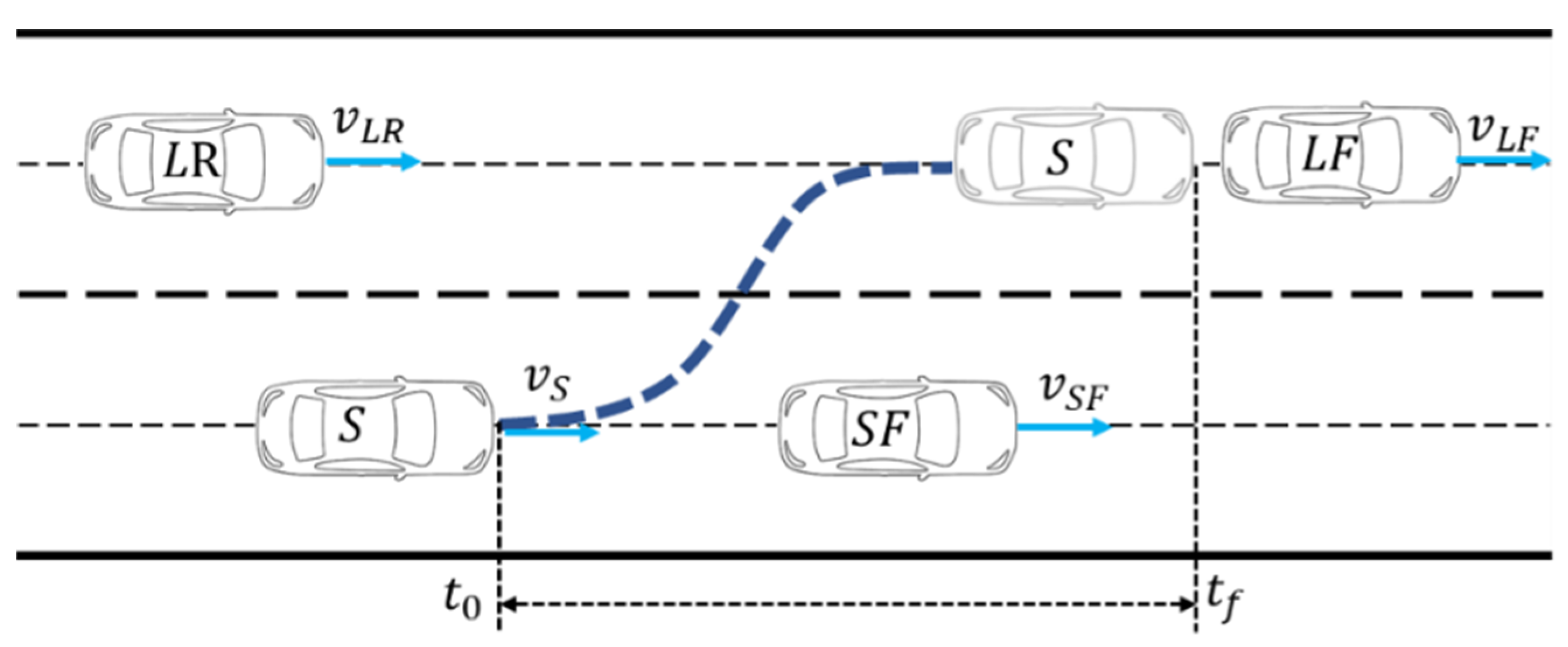
In the lane-changing scenario as shown in Figure 3, the ego vehicle is denoted as S with a velocity of v s . During the lane-changing process, the influences of three surrounding vehicles on the ego vehicle are considered. These vehicles are the front vehicle S F in the current lane, the front vehicle L F in the target lane, and the rear vehicle L R in the target lane. Their speeds are denoted as v S F , v L F , and v L R , respectively. The starting time of the lane-changing is denoted as t 0 , and the ending time is denoted as t f .
The shape of the lane-changing endpoint distribution area is a rectangle [28], as indicated by the dashed box in Figure 4. Within this region, the red dots represent possible lane-changing endpoints. The boundary of this area is defined as follows:
The upper boundary along the direction of vehicle travel is denoted as S u p , and the lower boundary along the direction of vehicle travel is denoted as S l o . The upper boundary perpendicular to the lane marking is denoted as L u p , and the lower boundary perpendicular to the lane marking is denoted as L l o . The calculation formulas for each boundary are as follows:
S u p = k 1 m a x { v S , v L F }
S l o = k 2 m i n { v S , v L F }
L u p = L l o = D s a f e
where k 1 and k 2 are lane-changing path adjustment coefficients that are related to the driver’s style. The values are smaller for aggressive drivers compared to conservative drivers. Typically, k 1 = 3 and k 2 = 6 . D s a f e represents the minimum safe distance that the vehicle maintains with road boundaries and lane markers. Usually, D s a f e = 0.3 .
(2)
Generation of candidate lane-changing paths
There are many types of geometric curves used to generate lane-changing paths. Different geometric curves require different input information and unknown parameters and result in different path qualities. In this paper, we adopt B-spline curves to generate lane-changing paths. The lane-changing paths generated using this method ensure curvature continuity, and the curvatures at the starting and ending points of the lane-changing match those of the reference path. Assuming we have P 0 ,   P 1 , P 2 ,   P n , as a set of n + 1 control points that define the direction and bounds of the spline curve, the definition of a k -th B-spline curve is as follows:
p ( u ) = [ P 0 ,   P 1 , P 2 ,   P n ] [ B 0 , k ( u ) B 1 , k ( u ) B n , k ( u ) ] = i = 0 n P i B i , k ( u )
where B i , k ( u ) represents the i -th k th-order B-spline basis function, corresponding to the control point P i . Here, k 1 , and u is the independent variable. The basis functions have the following recursive formula:
B i , 0 ( u ) = { 1 u [ u i , u i + 1 ) 0 u [ u i , u i + 1 )
B i , k ( u ) = u u i u i + k 1 u i B i , k 1 ( u ) + u i + k u u i + k u i + 1 B i + 1 , k 1 ( u )
where u i represents a set of continuously changing values known as the knot vector, which is a non-decreasing sequence. The initial and final values are typically defined as 0 and 1, respectively, that is, u 0 = 0 and u n + k = 1 . This sequence is denoted as [ u 0 , u 1 , , u k , u k + 1 , , u n , u n + 1 , , u n + k ] , and it satisfies u 0 u 1 u k u k + 1 u n u n + 1 u n + k . To alter the shape of the B-spline curve, one or more control parameters can be modified, such as the position of control points, the location of knots, or the degree of the curve.
The 4th-order quasi-uniform B-spline curve is used in this paper to generate lane-changing paths, as shown in Figure 5. By selecting six control points based on the lane-changing starting and ending points, a curvature-continuous lane-changing path can be generated, represented by points A, B, C, D, E, and F in Figure 5. The initial position of the vehicle at the lane-changing starting point is defined as point A, while any sampled point within the feasible region in Figure 4 can be chosen as the lane-changing endpoint, represented by point F. According to the characteristics of the quasi-uniform B-spline curve, when points A, B, and C, as well as D, E, and F, lie on the same line parallel to the lane centerline (i.e., ABC//DEF//lane centerline), it is possible to achieve zero curvature at the lane-changing starting and ending points. To ensure that the generated lane-changing path is symmetric about the centerline, it is required that ABC and DEF exhibit symmetric distributions. Therefore, by determining the positions of points B and C, a lane-changing path based on a 4th-order quasi-uniform B-spline curve can be generated. To ensure the optimality of the generated lane-changing path between the starting point A and the ending point F, this paper evaluates the quality of the lane-changing path using two metrics: path length and average curvature. Path length reflects the distance traveled during the lane-changing process, while average curvature represents the comfort of lateral vehicle control during the lane-changing process. By employing a multi-objective linear weighting approach, the lane-changing path evaluation function can be formulated as follows [29]:
C o s t p a t h = ω 1 i = 1 n 1 Δ d i , i + 1 + ω 2 i = 1 n κ i n
where ω 1 and ω 2 are the weighting coefficients of the sub-objective functions; Δ d i , i + 1 represents the distance between adjacent waypoints i and i + 1 in the lane-changing path; κ i denotes the curvature corresponding to waypoint i in the lane-changing path, which can be estimated assuming that three consecutive waypoints lie on the same circle; and n represents the number of waypoints included in the path.
By using a linear weighting approach, the combination of path length and average curvature is used as the optimization objective. Through an optimization algorithm, the positions of points B and C can be determined, thus selecting the six control points based on the lane-changing starting and ending points. Additionally, to simplify the optimization process and improve the efficiency of the path search, AB is set to be equal to AC, transforming the two-dimensional optimization problem into a one-dimensional optimization problem. Considering the differences in scale between path length and curvature, in the process of constructing the optimization objective, each of them is normalized and then combined through weighted summation to obtain the comprehensive optimization objective function.
Figure 6 shows the optimization results of lane-changing path control points under different weight distributions. It can be observed that with different weights, different path control points can be obtained, thereby affecting the shape of the generated lane-changing path when the starting and ending points of the lane-changing path are the same. When ω 1 = 0.1 and ω 2 = 0.9 , the optimal path control points correspond to AB = EF = 5.26   m and AC = DF = 10.52   m . When ω 1 = 0.9 and ω 2 = 0.1 , the optimal path control points correspond to AB = EF = 6.68   m and AC = DF = 13.36   m . When ω 1 = 0.6 and ω 2 = 0.4 , the optimal path control points correspond to AB = EF = 5.74   m and AC = DF = 11.48   m .
By using equidistant sampling within the possible region of lane-changing endpoints, multiple lane-changing target endpoints can be generated. Similarly, using the same approach, the candidate lane-changing paths can be generated, as shown by the solid red lines in Figure 4.
(3)
Collision checking for static obstacle
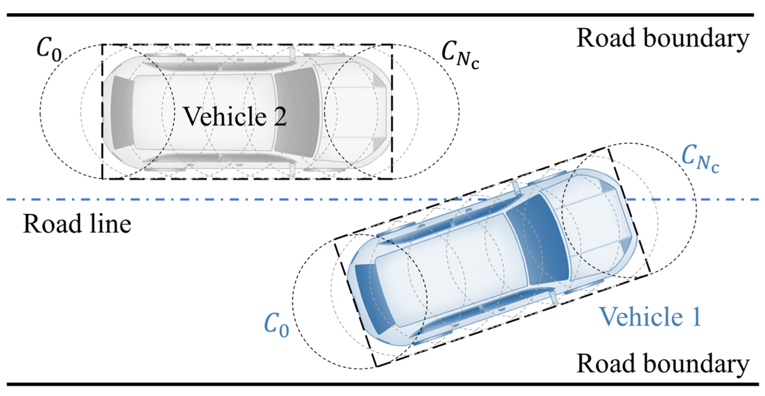
In this paper, the vehicle collision checking is performed using the dynamic circle envelope method. N c circles with the same radius are uniformly placed to cover the minimum bounding rectangle of the vehicle contour. The radius of the envelope circle is equal to half of the vehicle width. C 0 represents the envelope circle corresponding to the rear position of the vehicle, while C N c represents the envelope circle corresponding to the front position of the vehicle. The center coordinates of C 0 and C N c can be calculated based on the vehicle’s centroid position obtained from the vehicle positioning system and the vehicle’s size information. Let the center coordinates of C 0 and C N c be denoted as ( S C 0 , L C 0 ) and ( S C N c , L C N c ) , respectively. The calculation formula for the center coordinates of any envelope circle C i of the vehicle is as follows:
{ S i = S C 0 + λ N c 1 ( S C N c S C 0 ) L i = L C 0 + λ N c 1 ( L C N c L C 0 )
where λ is the independent variable defined on the interval [ 0 ,   N c 1 ] , and it is an integer.
The collision detection between two vehicles based on dynamic circular envelopes can be transformed into determining whether there is an overlapping region between any envelope circle covering the ego vehicle and any envelope circle covering the surrounding vehicles. The existence of overlap between two circles can be determined based on the distance between their centers. Therefore, in the scenario depicted in Figure 7, the collision detection condition between vehicle 1 and vehicle 2 can be represented as follows:
( S 1 S 2 ) 2 + ( L 1 L 2 ) 2 ( R 1 + R 2 ) 2
where S 1 and S 2 represent the S-axis coordinates of the centers of any enveloping circles for vehicle 1 and vehicle 2, respectively. L 1 and L 2 represent the L-axis coordinates of the centers of any enveloping circles for vehicle 1 and vehicle 2, respectively. R 1 and R 2 represent the radii of the envelope circles for vehicle 1 and vehicle 2, respectively, which are equal to half of the corresponding vehicle’s width.
Additionally, it is necessary to ensure that the vehicle remains within the boundaries of the road while driving along the planned waypoints. This can be achieved by checking whether there is an intersection between any envelope circle covering the vehicle and the lane boundaries.

3.1.3. Velocity Planning Using DP and QP

The task of velocity planning is to assign time-related information, such as speed, acceleration, etc., to the lane-changing waypoints, thereby completing the trajectory planning task.
(1)
Establishment of temporal and spatial graphs
  • 1.
    Trajectory prediction of surrounding vehicles
For lane-changing scenarios, considering that lane-changings typically occur over a short duration, a constant acceleration (CA) model in the Frenet coordinate system is often chosen to predict the motion trajectory of surrounding vehicles. In this model, the state variables of a vehicle include the longitudinal coordinate s , lateral coordinate l , heading angle θ (counterclockwise as positive) with respect to the S-axis, velocity v s , and acceleration a s , denoted as follows:
X C A = { s , l , θ , v s , a s }
If the sampling period is denoted as ∆T, then the vehicle state transition equation for the constant acceleration model can be expressed as follows:
X C A ( k + 1 ) = X C A ( k ) + ( ( v s Δ T + 1 2 a s Δ T 2 ) cos θ ( v s Δ T + 1 2 a s Δ T 2 ) sin θ 0 a s Δ T 0 )
According to this state transition equation, if the initial states of surrounding vehicles at the beginning of the lane-changing are known, the CA model can be used to obtain the predicted trajectories of surrounding vehicles within the prediction time domain.
  • 2.
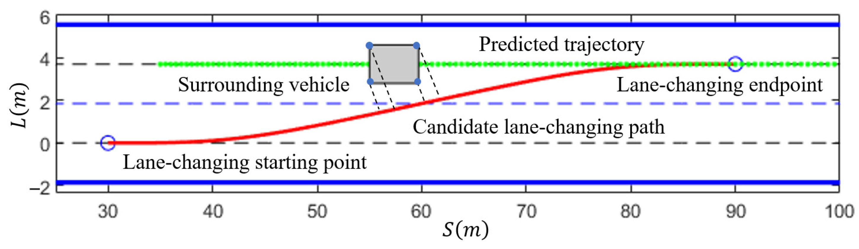
    Potential conflict detection for a lane-changing path
Based on whether there is an overlap between the predicted trajectories of surrounding vehicles and the candidate lane-changing paths generated in the previous steps, the potential conflict risk of the lane-changing path is determined. If there is no overlap between the predicted trajectories of surrounding vehicles and the lane-changing path, the velocity planning task does not need to consider the influence of that vehicle. However, if there is an overlap, it is necessary to conduct velocity planning for the lane-changing path to avoid the risk of collision with that vehicle. The method for assessing the potential conflict between the lane-changing path and surrounding vehicle A is as follows:
( S A S i ) 2 + ( L A L i ) 2 ( R 0 + R A ) 2
where ( S A , L A ) represents the coordinates of the center of any enveloping circle of surrounding vehicle A in the Frenet coordinate system, and ( S i , L i ) represents the coordinates of any point on the lane-changing path in the Frenet coordinate system. R 0 and R A , respectively, represent the radii of the enveloping circle of the ego vehicle and vehicle A, which are equal to half of the corresponding vehicle’s width.
If for any waypoint on the predicted trajectory of surrounding vehicle A and any point on the lane-changing path, the equation mentioned above is satisfied, there is no potential conflict between surrounding vehicle A and the ego vehicle. Conversely, if the equation is not satisfied, there is a potential conflict between surrounding vehicle A and the ego vehicle, and the velocity planning task needs to consider the influence of that vehicle, as shown in Figure 8a.
According to the aforementioned steps, the potential conflicts between the vehicle S F , vehicle L F , and vehicle L R with the ego vehicle are determined. The surrounding vehicles with conflicts are selected, and the starting time t 1 and ending time t 2 of the conflicts, as well as the coordinates of the corresponding roadway points in the Frenet coordinate system, are recorded. Any moment with a potential conflict is denoted as t k . The set of waypoints where the candidate lane-changing path and surrounding vehicles have potential conflicts is defined as the potential conflict zone Δ S t 
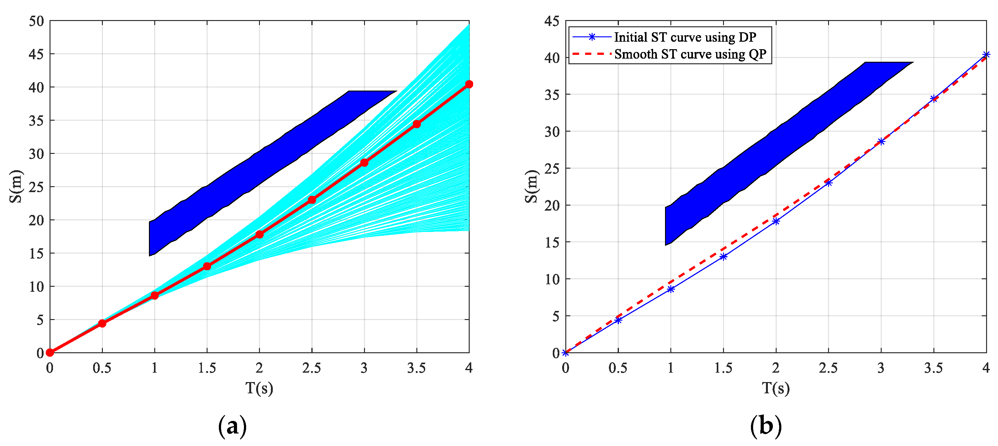
. All waypoints within the potential conflict zone at any moment of potential conflict are plotted in a coordinate system with time t as the horizontal axis and coordinate S in the Frenet coordinate system as the vertical axis, forming a temporal and spatial graph as shown in Figure 8b, commonly referred to as the ST graph. The slope of the curves in the ST graph can be used to determine the velocity trend: the steeper the slope, the faster the corresponding velocity. In Figure 8b, the solid red line represents the vehicle’s acceleration process, and the dashed blue line represents the vehicle driving at constant speed.
  • 3.
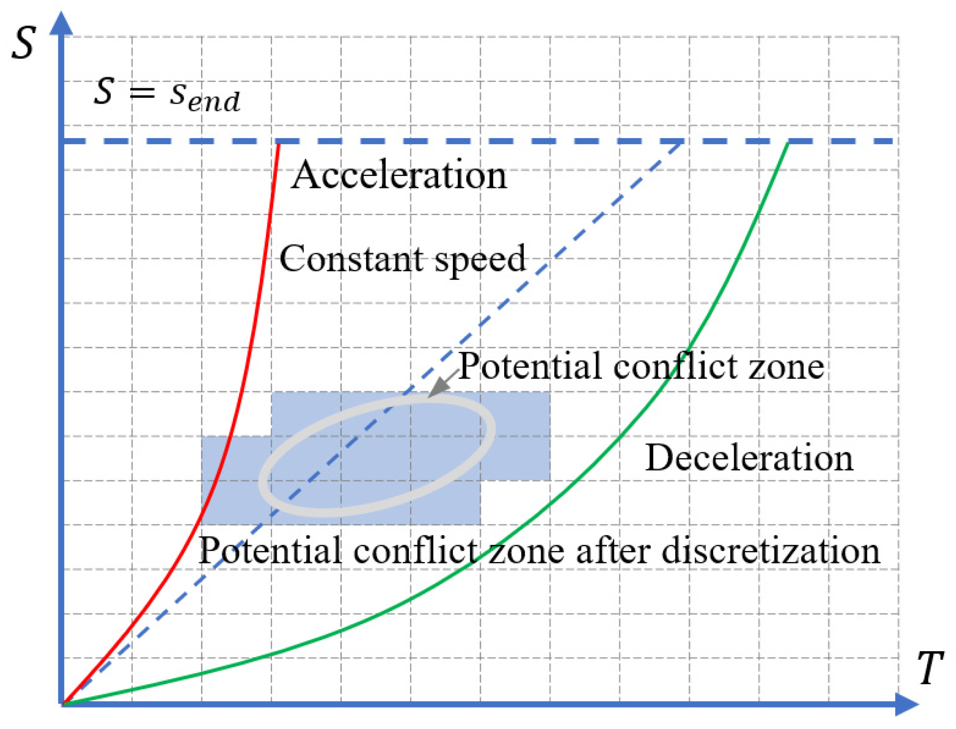
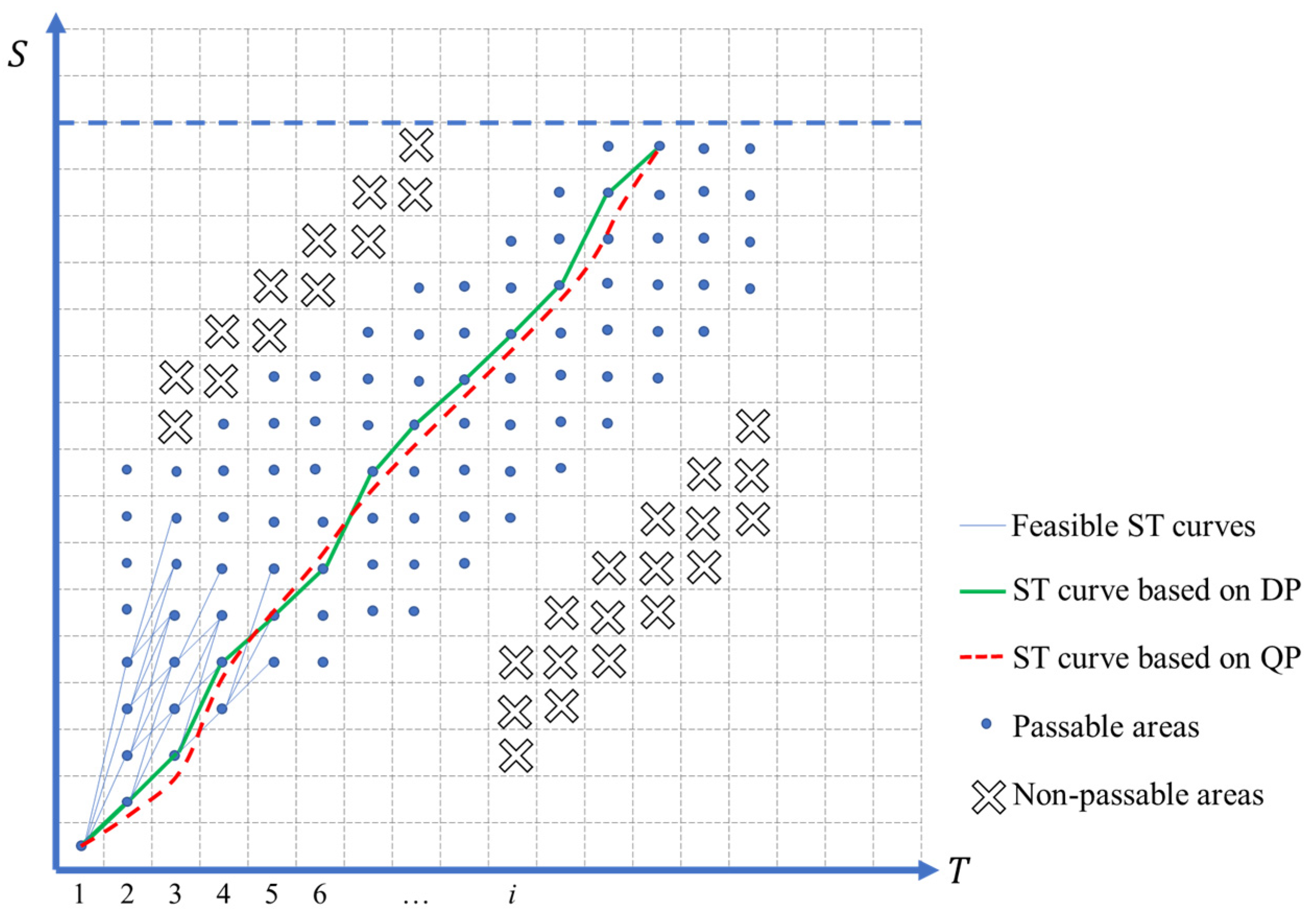
    Discretization of the temporal and spatial graph
To employ DP for velocity planning, the ST graph needs to be discretized. Based on calculation efficiency, planning time domain, and path length, an appropriate sampling interval is chosen to discretize the ST graph uniformly, as shown in Figure 9. It should be noted that the speed varies between cells but remains constant within each cell. The blue-shaded area in Figure 9 represents the potential conflict zone between the surrounding vehicle and the ego vehicle along the planned path in Figure 8a. Both the solid red line (vehicle acceleration for overtaking) and the dashed blue line (vehicle driving at a constant speed) overlap with the potential conflict zone, indicating unsafe velocity planning. The solid green line in the figure represents a velocity planning scheme that involves deceleration to avoid collisions with surrounding vehicles, meeting safety requirements.
(2)
Velocity generation and smoothing
The velocity planning process involves two steps: initial velocity generation and velocity smoothing.
  • 1.
    Velocity generation based on DP
The initial velocity generation method based on DP transforms the velocity planning problem into a multi-stage decision optimization problem using the discretized ST graph.
In each stage, the selectable S-axis coordinate position is related to the adjacent previous stage’s vehicle position, velocity, and maximum acceleration. In the discretized ST graph shown in Figure 9, the time series obtained by discretizing the horizontal axis with an equal interval Δ t are denoted as { t 0 , t 1 , t 2 , t 3 , , t n } , where t n is the end time of the lane-changing. The mileage sequence obtained by discretizing the vertical axis with equal intervals Δ s is denoted as S = { s 0 , s 1 , s 2 , s 3 , , s n } , where s n corresponds to the end point coordinate s end of the lane-changing. To evaluate the cost of the state transition, the velocity v i , acceleration a i , and jerk corresponding to state s i at stage i are calculated according to the following formulas:
v i = s ˙ i = s i s i 1 Δ t
a i = s ¨ i = s i + s i 2 2 s i 1 ( Δ t ) 2
j e r k i = s i = s i + s i 3 3 s i 1 3 s i 2 ( Δ t ) 3
The optimization objective function for initial velocity generation using DP is defined as follows:
C t o t a l ( S ) = ω D 1 C s m o o t h + ω D 2 C t a r g e t + ω D 3 C o b s ( S )
where ω D 1 , ω D 2 , and ω D 3 represent the weights of each sub-objective function. The first term of the objective function guarantees that the generated velocity is sufficiently smooth. The second term primarily aims to improve the efficiency of the lane-changing process, ensuring that the vehicle reaches the destination of the lane-changing as quickly as possible. The third term is mainly used to evaluate the distance between the ego vehicle and surrounding obstacle vehicles, ensuring safety.
The specific form of the objective function for smoothness, which is the first term, is as follows:
C s m o o t h ( S ) = ω 11 i = 0 n ( a i ) 2 + ω 12 i = 0 n ( j e r k i ) 2
The specific form of the objective function for efficiency, which is the second term, is as follows:
C t a r g e t ( S ) = i = 0 n ( s i s T ) 2
The specific form of the objective function for obstacle avoidance, which is the third term, is as follows:
C o b s ( S ) = i = 0 n C o b s ( s i )
C o b s ( s i ) = { i n f s o b s _ L ( i ) s i s o b s _ U ( i ) 0 s i s o b s _ U ( i ) + s s a f e _ o v e r t a k e 0 s i s o b s _ L ( i ) + s s a f e _ f o l l o w ( Δ s i s s a f e _ f o l l o w ) 2 0 s o b s L ( i ) s i s s a f e _ f o l l o w ( Δ s i s s a f e _ o v e r t a k e ) 2 0 s i s o b s _ U ( i ) s s a f e _ o v e r t a k e
where Δ s i represents the relative distance between the ego vehicle and surrounding obstacle vehicles. s s a f e _ o v e r t a k e is the minimum safe distance between the ego vehicle and the rear vehicle in the target lane during the overtaking process. It depends on the ego vehicle’s velocity and mass, and a recommended range is 50–100 m. s s a f e _ f o l l o w is the minimum safe distance between the ego vehicle and the front vehicle in the target lane during the following process. It also depends on the ego vehicle’s velocity and mass, and a recommended range is 50–100 m. s o b s _ L ( i ) and s o b s _ U ( i ) represent the minimum and maximum values of the potential conflict region between the ego vehicle and surrounding obstacle vehicles at stage i on the ST graph.
To improve the efficiency of velocity generation using DP, the state variable s ( i ) at stage i during the search process can be constrained by the following conditions:
s i > s i 1
v i < v m a x
a m i n a i a m a x
The first constraint ensures that the vehicle can only move forward and is not allowed to move backward. The second constraint states that the generated velocity must be lower than the vehicle’s maximum designed speed v m a x . The third constraint specifies that the vehicle’s acceleration cannot exceed the maximum acceleration capability of the vehicle.
The velocity generated through DP is optimal, but due to the discretization process, the resulting ST curve is represented as a piecewise linear curve, as shown by the solid green line in Figure 10. The slope of this curve represents the velocity, but the slope is not continuous. Therefore, further smoothing is required for the ST curve.
  • 2.
    Velocity smoothing based on QP
To generate a smooth velocity profile, a fifth-degree polynomial is used to connect adjacent state s ( i ) and s ( i + 1 ) obtained from the ST curve generated using DP. For the discrete ST curve composed of n states, the smoothed ST curve is formed by connecting the n 1 segments of fifth-degree polynomial curves. The expression for each segment of the polynomial curve is as follows:
s i ( t ) = a 0 , i + a 1 , i t + a 2 , i t 2 + a 3 , i t 3 + a 4 , i t 4 + a 5 , i t 5
v i ( t ) = a 1 , i + 2 a 2 , i t + 3 a 3 , i t 2 + 4 a 4 , i t 3 + 5 a 5 , i t 4
a i ( t ) = 2 a 2 , i + 6 a 3 , i t + 12 a 4 , i t 2 + 20 a 5 , i t 3
j e r k i ( t ) = 6 a 3 , i + 24 a 4 , i t + 60 a 5 , i t 2
The definition of the objective function for smoothing the ST curve includes three aspects: acceleration, jerk, and position error.
C t o t a l ( S ) = i = 0 n 1 [ ω S 1 t i 1 t i a i 2 ( t ) d t + ω S 2 t i 1 t i j e r k i 2 ( t ) d t + ω S 3 t i 1 t i ( s i ( t ) s i ) 2 d t ]
where ω S 1 , ω S 2 , and ω S 3 represent the weight coefficients of the sub-objective functions. t i 1 and t i represent the start and end times of the i-th segment of the fifth-degree polynomial curve. Since the ST curve generated through DP in the previous steps is uniformly sampled in the time dimension, the time period of each polynomial curve segment is equal, that is, t i t i 1 = Δ t .
The vehicle velocity smoothing problem based on QP includes three types of equality or inequality constraints, as described below.
First, there are equality constraints for the position, velocity, and acceleration at the connecting points between adjacent polynomial curves.
{ s i ( t ) = s i + 1 ( 0 ) v i ( t ) = v i + 1 ( 0 ) a i ( t ) = a i + 1 ( 0 )
Second, the first segment of the polynomial curve should satisfy the equality constraints for the starting position, velocity, and acceleration of the original ST curve.
{ s 1 ( 0 ) = s 0 v 1 ( 0 ) = v 0 a 1 ( 0 ) = a 0
Finally, all position points need to satisfy the corresponding maximum limit constraints for position, velocity, and acceleration.
{ s i ( t ) s o b s U ( i ) + s s a f e _ o v e r t a k e s i ( t ) s o b s _ L ( i ) s s a f e _ f o l l o w i n g v i ( t ) v m a x a m i n a i ( t ) a m a x
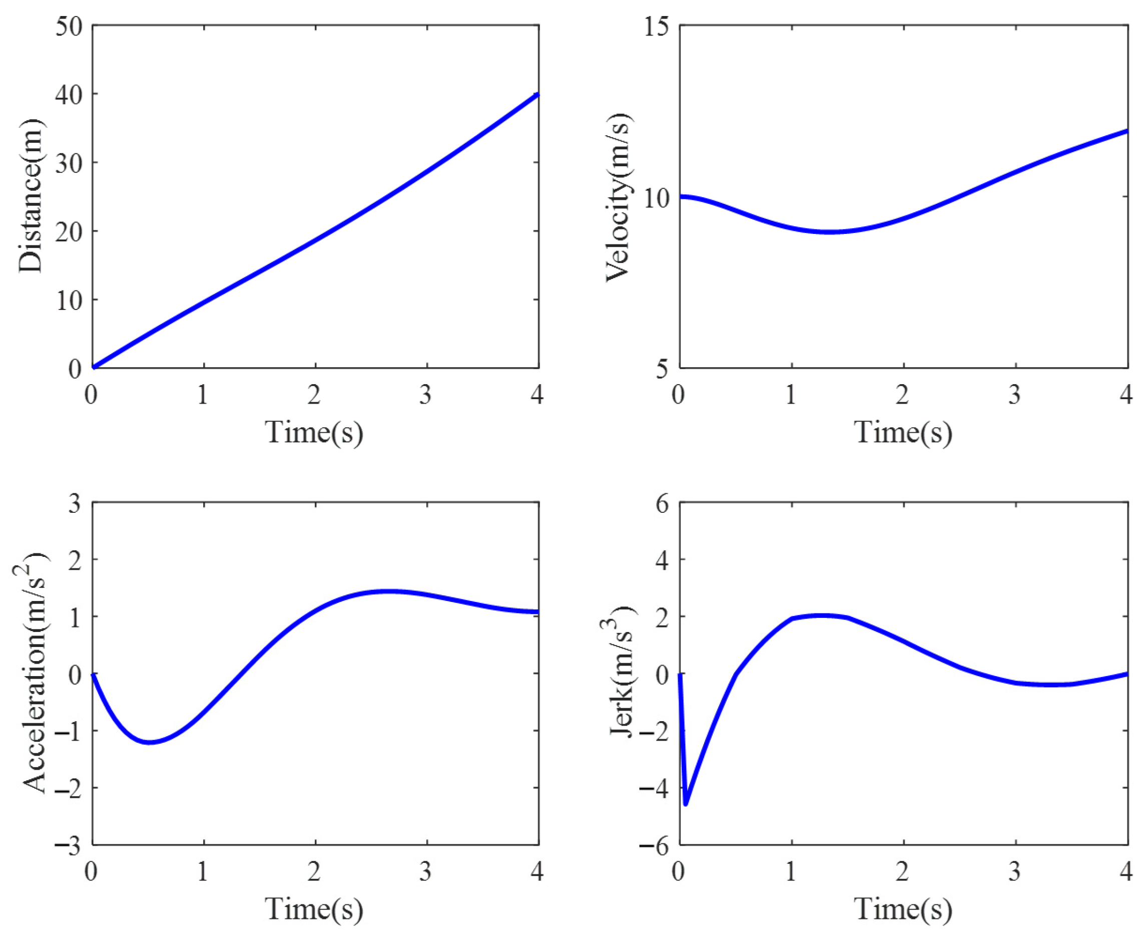
By combining the objective functions and constraints mentioned above, solving the QP problem will yield a smooth ST curve, which corresponds to a smooth velocity planning result. As shown in Figure 10, the red dashed line represents the ST curve obtained after smoothing.
(3)
Curvature checking of a lane-changing trajectory
The curvature check considers the minimum turning radius and prevents the vehicle from experiencing side slip during the turning process. First, the radius corresponding to the maximum curvature ρ m a x of the trajectory should be greater than the vehicle’s minimum turning radius R m i n . Second, to prevent side slip during the turning process, the lateral force during steering should not exceed the maximum available tire grip. Considering vehicle stability, the absolute value of the maximum lateral acceleration should be less than 0.4 g. Based on these considerations, the following constraint relationship between the trajectory curvature radius ρ and the planned vehicle speed v can be derived as follows:
| v 2 ρ | 0.4   g
By performing curvature checking on the lane-changing trajectory, candidate feasible lane-changing trajectories can be generated that satisfy the constraints of the minimum turning radius and prevent lateral slip from occurring.

3.2. Decision for Lane-Changing Target Trajectory

3.2.1. Definition of Trajectory Performance Evaluation Function

The Least Action Principle (LAP) is used to describe extremal phenomena in the natural world and physics. The actual motion or trajectory of objects in nature always minimizes the action, and for any stable state, there exists a corresponding minimum action. The term “action” refers to a cost measure of different motion choices that satisfies this principle. For example, when a rope hangs freely with both ends fixed, the system’s action, gravitational potential energy, tends to be minimized. In the problem of the fastest descent of a ball from a higher point to a lower point, time is the measure of action for this process. The significance of the Least Action Principle is that for every mechanical system, there exists an integral S called the action, which has a minimum value for the actual motion, that is →, variation δ S is zero. The authors of [27] discovered through statistical analysis of natural driving data that the main characteristic parameters reflecting driver decision-making behaviors during vehicle operation exhibit extremal phenomena. They conducted real-world experiments to verify that the driver decision-making mechanism follows the Least Action Principle, where drivers aim to achieve optimal maneuverability and safety while driving, pursuing the highest comprehensive performance while ensuring driving safety. They established the action of the driving process based on two dimensions: driving risk and travel time, and they defined the system’s Lagrangian function in the driving process as the difference between vehicle kinetic energy and potential energy. Therefore, this study aims to establish an action function for lane-changing trajectories based on two dimensions: driving risk and travel time, to objectively describe the driving goals pursued during the lane-changing process of intelligent vehicles.
(1)
Dynamic driving risk modeling based on the DSF
To ensure the safety of the lane-changing process, intelligent vehicles need to accurately assess the driving risks in the traffic environment and provide precise quantification of risk evaluation for real-time trajectory planning in dynamic and complex scenarios. Considering the similar characteristics between the risks generated by traffic factors and fields in physics [30], the concept of the driving safety field (DSF) is proposed to represent the risks generated by various elements of traffic to the driving vehicles on the road. The objects in the traffic scene that can cause driving risks can be mainly categorized into three types: human (drivers), vehicle (moving objects on the road), and road (static elements in the road environment). All traffic elements that pose driving risks to the vehicles on the road form a driving safety field, which repels other objects approaching it. Accordingly, the driving safety fields formed by these three types of objects are defined as the behavior field, kinetic field, and potential field, respectively.
This paper establishes a dynamic driving risk quantification evaluation model based on the theory of driving safety and illustrates the construction process of the dynamic driving risk quantification model using a lane-changing scenario as an example. For the lane-changing scenario shown in Figure 11, the driving risks are generated by the road boundaries, lane markers, and moving vehicles. First, we employ the potential field model proposed in Reference [30] to establish a risk field for the road boundaries and lane markers. Additionally, we use the kinetic field model from the same reference to establish risk fields for the moving vehicles. Next, we superimpose the risk field strengths generated by different traffic elements to obtain the comprehensive driving risk field for the lane-changing scenario, as depicted in Figure 11. Finally, considering the vehicle’s state and the road information at different time steps during the lane-changing process, we recalculate the distribution of the comprehensive driving risk field to obtain the dynamic driving risk distribution for the lane-changing process. Figure 11a shows the positional relationship between the ego vehicle and surrounding vehicles at the beginning of a lane change. Due to the presence of a stationary vehicle ahead in the current lane, the ego vehicle needs to select a different lane to avoid a collision. Before changing lanes, the ego vehicle needs to determine whether the target lane meets the lane-changing conditions based on perception information. It obtains the position and motion status of vehicles in the target lane and calculates the potential field formed by lane markings, the potential field formed by stationary vehicles, and the kinetic field of vehicles in the target lane based on the theory of driving safety field. The distribution of driving risk at the start of the lane-changing is shown in Figure 11a. From the figure, it can be observed that the current lane has higher risks ahead, while the target lane has lower risks. Moving the ego vehicle to a low-risk area through lane-changing improves driving safety. Figure 11b shows the motion trajectories of the ego vehicle and the following vehicles in the target lane during the lane-changing process, as well as the distribution of driving risk after the lane-changing is completed. During the lane-changing process, the relative positions of the ego vehicle to the preceding stationary vehicle and the following vehicles in the target lane are dynamically changing. The magnitudes and directions of the driving safety field formed by various traffic participants are also dynamically changing, resulting in the low-risk area available for the ego vehicle to drive also changing with time and space. Therefore, in the trajectory planning process of lane-changing, this paper constructs a dynamic driving risk model based on real-time position and attitude information of the ego vehicle and various traffic participants to ensure the safety of the planned trajectory.
(2)
Definition of the evaluation function based on the LAP
According to the definition of the Least Action Principle, the action of the lane-changing process for vehicles can be defined as follows:
S R i s k = t 0 t f L i d t
L i = T i U i
where S R i s k represents the action of the vehicle during the lane-changing process along the planned trajectory. t 0 is the starting time of the lane-changing, and t f is the ending time of the lane-changing. L i is the system Lagrangian during the lane-changing process. T i and U i represent the kinetic and potential energies of the vehicle, respectively. U i is the sum of the safety potential energies that the vehicle possesses while driving in the driving safety field generated by stationary and moving obstacles.
T i = 1 2 m v i 2
where m represents the mass of the ego vehicle and v i represents the corresponding vehicle speed of the ego vehicle during the lane-changing process along the planned trajectory.
U i = j = 1 K t 0 t f F i j ( v i v j ) d t
where K represents the number of surrounding vehicles around the ego vehicle. For the scenario shown in Figure 1, K = 3 . v j represents the speed of the surrounding vehicle j of the ego vehicle. F i j represents the interaction force exerted on the ego vehicle in the risk field generated by the surrounding vehicle   j .
F i j = E i j · m · R O = K · T j · R O · M j · m · e ( k D 2 · v i j · cos ( θ D o ) ) | r j o | k D 1
where E i j represents the strength of the driving risk field generated by the surrounding vehicle j (dynamic obstacle) at the position of the ego vehicle. The calculation formula can be found in reference [30]. R O is the influencing factor of road adhesion at the position of the ego vehicle, which is related to the road adhesion coefficient determined by the road surface and tires. When the adhesion rate C φ of the driving wheels is less than or equal to the road adhesion coefficient φ , R O = 1 . When the adhesion rate C φ of the driving wheels is greater than the road adhesion coefficient φ , R O = f ( C φ φ ) and R O > 1 . The larger the value of | C φ φ | , the larger the value of R O . | r j o | is the distance from the centroid position of surrounding vehicle j to the position of the ego vehicle. M j is the mass of the surrounding vehicle j . T j is the influencing factor of the risk magnitude of the surrounding vehicle j , which is related to the size of the moving obstacle. It is obvious that trucks have larger values of T j compared to passenger cars, and T j > 1 . Generally, T j falls within the range of [1, 10]. For example, T j is 1 for passenger cars and 3 for trucks. K , k D 1 , and k D 2 are constants. Typically, K = 1 , k D 1 falls within the range of [1, 10], and k D 2 falls within the range of [0.01, 0.1]. v i j represents the magnitude of the relative velocity between the ego vehicle and surrounding vehicle j . θ D o represents the angle between the motion velocity of the ego vehicle and the surrounding vehicle j .

3.2.2. Selection of Lane-Changing Trajectory

The lane-changing trajectory decision is primarily based on the trajectory evaluation results to select a target one from the candidate lane-changing trajectories. For any feasible candidate lane-changing trajectory, the actual action S Risk of the vehicle during the lane-changing process is calculated. Considering the differences in lane-changing duration for different trajectories, this paper defines the average action as a measure of lane-changing trajectory quality. The average action is defined as the ratio of the actual action of the lane-changing trajectory to the lane-changing duration, and the calculation formula is as follows:
S A v e = S R i s k t f t 0
According to the average action of the lane-changing trajectories, all feasible candidate lane-changing trajectories are sorted, and the trajectory with the smallest average action is selected for moving obstacle checking. If the collision checking fails, the trajectory is excluded, and the decision process continues by selecting the candidate trajectory with the next smallest average action quantity for collision checking. This continues until a collision-free trajectory is chosen as the final output of the lane-changing trajectory planning.

3.2.3. Collision Checking for Moving Obstacles

Collision checking for moving obstacles is carried out to ensure the safety of the selected lane-changing trajectory. It mainly focuses on collision-checking between the ego vehicle and surrounding moving vehicles. The same method as static obstacle collision checking is employed. The process involves sequentially checking whether the ego vehicle’s movement along the selected lane-changing trajectory with the smallest average action satisfies the collision checking requirements with the surrounding moving vehicles.

4. Simulation Analysis and Discussion

The proposed hierarchical trajectory planning method in this paper was validated using the MATLAB 2021a simulation platform. Two types of scenarios were set up: lane-changing overtaking and lane-changing following. The trajectory algorithm involves multiple optimization models, including lane-changing path optimization based on B-spline curves, ST curve optimization based on DP, and ST curve smoothing based on QP. These optimization problems are all typical multi-objective optimization problems. In this paper, a weighted sum approach was used to transform the objectives into single-objective optimization problems. The weight coefficients of the sub-objective functions for each optimization problem are shown in Table 1.
The lane-changing scenario, as shown in Figure 12, was constructed for algorithm validation in this paper. The scenario consists of a single-direction dual-lane with curved arcs. The thick, solid blue line represents the road boundary, the dashed blue line represents the lane markings, and the dashed black line represents the lane centerline. To facilitate the subsequent scenario description, a Frenet coordinate system was established with the red asterisk in the figure as the origin. The lane-changing scenario depicted in Figure 12a was transformed to the Frenet coordinate system. The curved lane-changing scenario in the Cartesian coordinate system was converted to a straight lane-changing scenario in the Frenet coordinate system, as shown in Figure 12b. The figure demonstrates the transformation of the lane-changing path (red solid line) from the Cartesian coordinate system to the Frenet coordinate system (red solid line).

4.1. Simulation Scenario 1: Lane-Changing and Following

Figure 13a depicts the lane-changing and following scenario. At the beginning of the lane-changing, there is a stationary vehicle (obstacle) ahead of the ego vehicle in the current lane. The ego vehicle needs to perform the lane-changing to avoid collision with the stationary vehicle and, after the lane-changing, follow the moving vehicles in the target lane. The initial parameters of each vehicle at the start time are provided in Table 2. The ego vehicle has an initial velocity of 10 m/s with an acceleration of 0. The distance between the ego vehicle and the leading obstacle vehicle on the current lane is 30 m. The leading vehicle, LF, on the target lane has an initial velocity of 10 m/s with an acceleration of 0.5 m/s2, moving with constant acceleration. The requirements for the lane-changing process are to avoid collision with the vehicle SF and maintain an appropriate following distance with the leading vehicle, LF, on the target lane. The vehicle’s heading angle should align with the centerline of the lane at the beginning and end of the lane-changing.
Based on the proposed lane-changing endpoint selection method and the lane-changing requirements of the scenario, the lane-changing endpoint is selected on the centerline of the target lane. The range of the longitudinal position for the lane-changing endpoint is set with a minimum distance of 30 m from the ego vehicle’s current position and a maximum distance of 60 m. The endpoints for the lane-changing are generated by sampling at 5 m intervals, as shown by the blue circles in Figure 14. The red circle represents the lane-changing starting point, the blue square represents the ego vehicle, and the gray squares represent the vehicles LF and SF in the scenario depicted in Figure 13a. The candidate lane-changing paths generated using a fourth-order quasi-uniform B-spline curve are shown by the red solid line in Figure 14.
Selecting any one from the candidate lane-changing paths, its curvature and heading angle in the Cartesian coordinate system are analyzed, as shown in Figure 15. The red dashed line represents the curvature of the road centerline, while the blue solid line represents the curvature of the planned path. The curvature at the beginning and end of the lane-changing matches the curvature of the road centerline, satisfying the requirement for the vehicle to travel along the centerline before and after the lane-changing. Additionally, from the path heading angle with respect to distance, it can be observed that the vehicle’s heading angle varies continuously along the planned path. This would provide continuous control targets for the vehicle’s trajectory tracking.
The CA model is used to obtain the predicted trajectory of vehicle LF for the next 6 s, as shown by the green dashed line in Figure 16. The four vertices of LF’s minimum-bounding rectangle are projected onto the lane-changing path. By comparing the shortest distance between the four vertices and the lane-changing path with the minimum safety distance between vehicles, the presence of a collision risk between the ego vehicle and LF is determined. If there is potential collision risk, the length of LF occupying the lane-changing path is projected onto the ST graph. Throughout the lane-changing process, the intervals where vehicle LF and the ego vehicle have potential collision risk on the lane-changing path are projected onto the ST graph, resulting in the blue-shaded area shown in Figure 17. The ST graph is discretized with a time sampling interval of 0.5 s on the horizontal axis and a distance sampling interval of 0.2 m on the vertical axis, creating the search space for velocity generation using DP. Figure 17a illustrates the initial velocity generation process for the lane-changing path. The cyan solid line represents the feasible velocity sequence from the lane-changing starting point to the endpoint. Based on the objective function and constraints, the red solid line represents the optimal ST curve obtained through DP, and the solid red dots represent the optimal state at each stage. It can be observed that the ST curve consists of line segments, resulting in non-smooth velocity. After applying the proposed smoothing method, the smoothed velocity curve is obtained, as shown by the red dashed line in Figure 17b.
Figure 18 shows the variation of distance, velocity, acceleration, and jerk over time for the lane-changing trajectory planned using the proposed method. It can be seen that during the lane-changing and following processes, the ego vehicle first decelerates to ensure that the distance between the ego vehicle and vehicle LF meets the safety requirements after the lane-changing. Once the spacing between the two vehicles reaches the safe following distance, the ego vehicle starts accelerating to the target speed for following, ensuring a quick completion of the lane-changing process. The acceleration during the entire lane-changing process is continuous and smooth, with a maximum jerk of less than 5 m / s 3 , which can improve the driving comfort during the lane-changing process.
According to the proposed trajectory quality evaluation function in this paper, the actual action is calculated for the candidate lane-changing trajectories. Table 3 shows the lane-changing durations for seven candidate trajectories, with a maximum duration of 5.65 s and a minimum duration of 3 s. Considering the time differences among different trajectories, we evaluate the quality of the trajectories based on the average action. The average action is defined as the ratio of the actual action of the trajectory to the lane-changing duration. Figure 19 shows the comparison of average action for the seven candidate trajectories in the lane-changing and following scenario. From the figure, it can be observed that the second trajectory has the smallest average action. The lane-changing endpoint coordinate of this trajectory is (65, 3.7). After the moving obstacle collision checking, the second trajectory is ultimately selected as the target lane-changing trajectory with the best comprehensive performance and alignment with driver characteristics. By adopting a weighted cost function similar to the one in reference [22], we selected three evaluation metrics, namely trajectory length, trajectory curvature, and lane-changing duration, to construct a multi-objective cost for assessing trajectory quality. The weights of the three sub-objective functions are denoted as ω c 1 , ω c 2 , and ω c 3 , respectively. When ω c 1 = 1 , ω c 2 = 2 , and ω c 3 = 10 , the evaluation results of trajectory quality are shown as the black-dashed line in Figure 19, where the 7th trajectory has the minimum total cost and is considered the optimal trajectory. When ω c 1 = 2 , ω c 2 = 1 , and ω c 3 = 10 , the evaluation results of trajectory quality are shown as the red-dashed line in Figure 19, where the 3rd trajectory has the minimum total cost and is considered the optimal trajectory. It can be observed that slight variations in the weights will result in changes in the trajectory selection outcomes. Furthermore, the allocation of weights is subjective, and a single-weighted objective function is difficult to adapt to complex scenarios. However, the evaluation metrics proposed in this paper do not require consideration of weight allocation issues and can adapt to dynamic environments by selecting reasonable trajectories that meet the driver’s requirements.
To further validate the effectiveness of the hierarchical planning method proposed in this paper, the trajectory tracking control method based on model predictive control (MPC) proposed in reference [31] is employed to analyze the lateral and longitudinal errors of the vehicle tracking the planned lane-changing trajectory. Figure 20a shows the results of the error analysis during the trajectory tracking process. It can be observed that the maximum lateral tracking error is less than 0.01 m, the heading angle tracking error is less than 0.02 rad, and the velocity tracking error does not exceed 0.2 m/s. These errors satisfy the requirements for trajectory tracking, indicating that the vehicle can successfully track the planned lane-change trajectory and complete the lane-change process effectively.

4.2. Simulation Scenario 2: Lane-Changing and Overtaking

Figure 13b shows the lane-changing and overtaking scenario. At the beginning, there is a stationary vehicle (obstacle) ahead of the ego vehicle in the current lane. The ego vehicle needs to perform the lane-changing to avoid a collision with the stationary vehicle. As there is a moving vehicle behind the target lane, the ego vehicle needs to overtake the vehicle after completing the lane-changing. The initial parameters of each vehicle at the starting time are shown in Table 4. The ego vehicle has an initial velocity of 10 m/s and an acceleration of 0. The distance between the obstacle vehicle and the ego vehicle in the longitudinal direction is 30 m. The target lane’s rear vehicle LR has an initial velocity of 10 m/s and an acceleration of 0.5 m/s2, moving with constant acceleration. The requirements for the ego vehicle during the lane-changing process are to avoid a collision with the front vehicle SF and maintain an appropriate safe distance with the rear vehicle LR in the target lane. At the start and end times of the lane-changing, the ego vehicle’s heading angle is required to align with the centerline of the lane.
Similar to Scenario 1, the lane-changing endpoint is selected on the centerline of the target lane. The range of longitudinal positions for the lane-changing endpoint is determined by the minimum longitudinal distance of 30 m from the current position of the ego vehicle as the lower bound and the maximum longitudinal distance of 60 m as the upper bound. The lane-changing endpoints are generated by sampling at intervals of 5 m, as shown by the blue circles in Figure 21. The red circle represents the lane-changing starting point, the blue square represents the ego vehicle, and the gray squares represent the vehicles LR and SF in the scenario depicted in Figure 13b. The candidate paths generated using fourth-order quasi-uniform B-spline curves are shown by the red solid line in Figure 21.
Since the lane-changing endpoints in Scenario 2 are the same as in Scenario 1, the planned lane-changing paths are also the same as in Scenario 1. The path has continuous curvature, and the curvature of the lane-changing starting and endpoint aligns with the road centerline. However, the same lane change path in two different scenarios results in differences in the ST graph established due to variations in the positions and motion states of the surrounding vehicles relative to the ego vehicle. The blue-shaded area in Figure 22 represents the projection of a potential conflict region between the predicted trajectory of vehicle LR and the lane-changing path on the ST graph. Comparing it with the ST graph shown in Figure 17, it can be observed that the positions and motion states of the surrounding vehicles can affect the feasible space for ego vehicle velocity planning. Therefore, even though the lane-changing paths are the same in Scenario 1 and Scenario 2, the velocity planning is different. Figure 22 illustrates the velocity planning process for the candidate path with an endpoint of (70, 3.7). In Figure 22a, the thin solid cyan line represents the feasible ST curve from the starting point to the endpoint. The red solid line represents the optimal ST curve obtained by DP based on the defined cost function and constraints. The solid red dots represent the optimal states at each stage. It can be seen that the optimal ST curve reaches the lane-changing endpoint at 3.5 s, indicating that the lane-changing and overtaking process can be completed in just 3.5 s. Additionally, it can be observed that the optimal ST curve is a polyline, resulting in non-smooth velocity. After applying the smoothing method proposed in this paper, the smoothed velocity is obtained, as shown by the red dashed line in Figure 22b.
Figure 23 shows the variations of distance, velocity, acceleration, and jerk of the trajectory over time. After the ego vehicle changes lanes, it needs to maintain a safe distance from the trailing vehicle in the target lane. Starting from the lane change initiation, the ego vehicle needs to increase the spacing with the trailing vehicle through acceleration. When the distance between the two vehicles exceeds the safety threshold and does not affect the normal driving of the trailing vehicle, the ego vehicle continues to maintain a higher velocity to ensure a safe and efficient completion of the lane-changing and overtaking processes. It can be observed that the velocity sequence obtained through DP and QP meets the requirements of lane-changing and overtaking. The acceleration of the ego vehicle changes continuously and smoothly, and the maximum acceleration and jerk satisfy the limit constraints. Table 5 presents the lane-changing duration for the candidate trajectory in Scenario 2. Comparing it with Table 3, it can be seen that for the same path, lane-changing and overtaking require less time compared to lane-changing and following.
Figure 24 shows the comparison of the average action for the seven candidate trajectories in the lane-changing and overtaking scenario. It can be observed that the sixth trajectory has the smallest average action. The lane-changing endpoint coordinate of this trajectory is (85, 3.7). After the moving obstacle collision checking, the sixth trajectory is ultimately chosen as the target lane-changing trajectory with the best comprehensive performance and alignment with driver characteristics. Similar to Scenario 1, we also select three evaluation metrics, namely trajectory length, trajectory curvature, and lane change duration, to construct a multi-objective evaluation function. The weights of the three sub-objective functions are denoted as ω c 1 , ω c 2 , and ω c 3 , respectively. When ω c 1 = 1 , ω c 2 = 2 , and ω c 3 = 10 , the evaluation results of trajectory quality are shown as the black dashed line in Figure 24, where the 7th lane change trajectory has the minimum total cost and is considered the optimal trajectory. When ω c 1 = 2 , ω c 2 = 1 , and ω c 3 = 10 , the evaluation results of trajectory quality are shown as the red dashed line in Figure 24, where the 1st lane change trajectory has the minimum total cost and is considered the optimal trajectory. This further verifies the advantages of the proposed method over the weighted objective function evaluation method, which can be used to solve local trajectory planning problems in complex environments.
Similar to Scenario 1, Figure 20b shows the analysis results of the tracking errors during the lane-change and overtaking processes. It can be seen that the maximum lateral tracking error is less than 0.01 m, the heading angle tracking error is less than 0.02 rad, and the speed tracking error does not exceed 0.5 m/s. These errors satisfy the requirements for trajectory tracking, indicating that the vehicle can successfully track the planned lane-change trajectory and complete the lane-change process effectively.

5. Conclusions

Intelligent vehicles have significant implications for enhancing driving safety, improving travel efficiency, alleviating traffic congestion, and enhancing driving comfort. This paper focuses on the research of lane-changing trajectory planning methods for autonomous driving, aiming to achieve reliable real-time avoidance of obstacles in multi-vehicle interaction scenarios. Existing studies primarily rely on quantitative comparisons using evaluation metrics and functions. However, the diversity of evaluation metrics introduces issues such as subjective weight allocation, preference bias, and poor robustness. To address these challenges, we propose a hierarchical lane-changing trajectory planning method based on the Least Action Principle (LAP).
Our method uses a path-velocity decomposition approach, follows the decision-making mechanism of excellent drivers, and establishes a comprehensive evaluation function considering safety, comfort, and efficiency. This enables multi-objective optimal decision-making for lane-changing trajectory selection.
We validate the effectiveness of our proposed method through experiments on two common lane-change scenarios. The proposed method automatically adjusts the lane-changing endpoint area based on surrounding dynamic traffic information, improving adaptability. It optimizes candidate paths, performs obstacle checking before speed planning, and combines DP and QP for vehicle velocity planning. This reduces speed variations during the lane-changing process and enhances driving comfort. The integration of a multi-objective optimal evaluation function, inspired by excellent drivers’ decision-making mechanisms, generates safe, smooth, and efficient lane-changing trajectories for different scenarios.
Future research will involve testing and evaluating our proposed method in various scenarios using autonomous vehicles. We will compare our method with lane-changing trajectories of multiple driver types in complex scenarios, including fixed and variable curvature, and challenging conditions to further validate its superiority.

Author Contributions

Investigation, K.L. and Y.F.; methodology, K.L., G.W. and Y.F.; validation, K.L. and G.W.; writing, K.L. and H.W. All authors have read and agreed to the published version of the manuscript.

Funding

This research was supported by the National Natural Science Foundation of China (Grant No. 52102463) and the Foundation of the State Key Laboratory of Automotive Simulation and Control (No. 20210231).

Data Availability Statement

Data are contained within the article.

Conflicts of Interest

The authors declare no conflicts of interest.

References

  1. Nastjuk, I.; Herrenkind, B.; Marrone, M.; Brendel, A.B.; Kolbe, L.M. What drives the acceptance of autonomous driving? An investigation of acceptance factors from an end-user’s perspective. Technol. Forecast. Soc. Chang. 2020, 161, 120319. [Google Scholar] [CrossRef]
  2. Li, X.; Sun, Z.; Cao, D.; Liu, D.; He, H. Development of a new integrated local trajectory planning and tracking control framework for autonomous ground vehicles. Mech. Syst. Signal Proc. 2017, 87, 118–137. [Google Scholar] [CrossRef]
  3. Yuan, Z.; Wang, Z.; Li, X.; Li, L.; Zhang, L. Hierarchical Trajectory Planning for Narrow-Space Automated Parking with Deep Reinforcement Learning: A Federated Learning Scheme. Sensors 2023, 23, 4087. [Google Scholar] [CrossRef] [PubMed]
  4. Ziegler, J.; Bender, P.; Schreiber, M.; Lategahn, H.; Strauss, T.; Stiller, C.; Dang, T.; Franke, U.; Appenrodt, N.; Keller, C.G. Making bertha drive—An autonomous journey on a historic route. IEEE Intell. Transp. Syst. Mag. 2014, 6, 8–20. [Google Scholar] [CrossRef]
  5. Kant, K.; Zucker, S.W. Toward efficient trajectory planning: The path-velocity decomposition. Int. J. Robot. Res. 1986, 5, 72–89. [Google Scholar] [CrossRef]
  6. González, D.; Pérez, J.; Milanés, V.; Nashashibi, F. A review of motion planning techniques for automated vehicles. IEEE Trans. Intell. Transp. Syst. 2015, 17, 1135–1145. [Google Scholar] [CrossRef]
  7. Sun, Y.; Yang, J.; Zhao, D.; Shu, Y.; Zhang, Z.; Wang, S. A Global Trajectory Planning Framework Based on Minimizing the Risk Index. Actuators 2023, 12, 270. [Google Scholar] [CrossRef]
  8. Li, H.; Zhao, T.; Dian, S. Forward search optimization and subgoal-based hybrid path planning to shorten and smooth global path for mobile robots. Knowl. -Based Syst. 2022, 258, 110034. [Google Scholar] [CrossRef]
  9. Jeong, I.; Lee, S.; Kim, J. Quick-RRT*: Triangular inequality-based implementation of RRT* with improved initial solution and convergence rate. Expert Syst. Appl. 2019, 123, 82–90. [Google Scholar] [CrossRef]
  10. Li, Q.; Xu, Y.; Bu, S.; Yang, J. Smart vehicle path planning based on modified PRM algorithm. Sensors 2022, 22, 6581. [Google Scholar] [CrossRef]
  11. Liu, Y.; Zhou, B.; Wang, X.; Li, L.; Cheng, S.; Chen, Z.; Li, G.; Zhang, L. Dynamic lane-changing trajectory planning for autonomous vehicles based on discrete global trajectory. IEEE Trans. Intell. Transp. Syst. 2021, 23, 8513–8527. [Google Scholar] [CrossRef]
  12. Van Hoek, R.; Ploeg, J.; Nijmeijer, H. Cooperative driving of automated vehicles using B-splines for trajectory planning. IEEE Trans. Intell. Veh. 2021, 6, 594–604. [Google Scholar] [CrossRef]
  13. Gutjahr, B.; Gröll, L.; Werling, M. Lateral vehicle trajectory optimization using constrained linear time-varying MPC. IEEE Trans. Intell. Transp. Syst. 2016, 18, 1586–1595. [Google Scholar] [CrossRef]
  14. Dixit, S.; Montanaro, U.; Dianati, M.; Oxtoby, D.; Mizutani, T.; Mouzakitis, A.; Fallah, S. Trajectory planning for autonomous high-speed overtaking in structured environments using robust MPC. IEEE Trans. Intell. Transp. Syst. 2019, 21, 2310–2323. [Google Scholar] [CrossRef]
  15. Yang, W.; Chen, Y.; Su, Y. A Double-Layer Model Predictive Control Approach for Collision-Free Lane Tracking of On-Road Autonomous Vehicles. Actuators 2023, 12, 169. [Google Scholar] [CrossRef]
  16. Jeong, Y.; Yim, S. Model predictive control-based integrated path tracking and velocity control for autonomous vehicle with four-wheel independent steering and driving. Electronics 2021, 10, 2812. [Google Scholar] [CrossRef]
  17. Wang, J.; Wu, J.; Zheng, X.; Ni, D.; Li, K. Driving safety field theory modeling and its application in pre-collision warning system. Transp. Res. Pt C-Emerg. Technol. 2016, 72, 306–324. [Google Scholar] [CrossRef]
  18. Sattel, T.; Brandt, T. From robotics to automotive: Lane-keeping and collision avoidance based on elastic bands. Veh. Syst. Dyn. 2008, 46, 597–619. [Google Scholar] [CrossRef]
  19. Werling, M.; Kammel, S.; Ziegler, J.; Gröll, L. Optimal trajectories for time-critical street scenarios using discretized terminal manifolds. Int. J. Robot. Res. 2012, 31, 346–359. [Google Scholar] [CrossRef]
  20. Li, T.; Wu, J.; Chan, C.; Liu, M.; Zhu, C.; Lu, W.; Hu, K. A cooperative lane change model for connected and automated vehicles. IEEE Access 2020, 8, 54940–54951. [Google Scholar] [CrossRef]
  21. Zhou, H.; Hu, X.; Chen, L.; Tian, M.; Xiong, D. Dynamic path planning for autonomous driving with avoidance of obstacles. J. Comput. Appl. 2017, 37, 883. [Google Scholar]
  22. Hu, X.; Chen, L.; Tang, B.; Cao, D.; He, H. Dynamic path planning for autonomous driving on various roads with avoidance of static and moving obstacles. Mech. Syst. Signal Proc. 2018, 100, 482–500. [Google Scholar] [CrossRef]
  23. Fu, X.; Jiang, Y.; Huang, D.; Wang, J.; Huang, K. Intelligent computing budget allocation for on-road trajectory planning based on candidate curves. Front. Inform. Technol. Electron. Eng. 2016, 17, 553–565. [Google Scholar] [CrossRef]
  24. Mcnaughton, M. Parallel Algorithms for Real-Time Motion Planning; Carnegie Mellon University: Pittsburgh, PA, USA, 2011. [Google Scholar]
  25. Dong, Q.; Yan, Z.; Nakano, K.; Ji, X.; Liu, Y. Graph-based Scenario-Adaptive Lane-Changing Trajectory Planning for Autonomous Driving. IEEE Robot. Autom. Lett. 2023, 8, 5688–5695. [Google Scholar] [CrossRef]
  26. Jurecki, R.S.; Stańczyk, T.L. Modelling Driver’s Behaviour While Avoiding Obstacles. Appl. Sci. 2023, 13, 616. [Google Scholar] [CrossRef]
  27. Wang, J.; Zheng, X.; Huang, H. Decision-making Mechanism of the Drivers Following the Principle of Least Action. China J. Highw. Transp. 2020, 33, 155. [Google Scholar]
  28. Ying, W.; Chong, W.; Lu, M. Dynamic lane-changing trajectory planning model for intelligent vehicle based on quadratic programming. China J. Highw. Transp. 2021, 34, 79. [Google Scholar]
  29. Wang, J.; Yuan, X.; Liu, Z.; Tan, W.; Zhang, X.; Wang, Y. Adaptive Dynamic Path Planning Method for Autonomous Vehicle Under Various Road Friction and Speeds. IEEE Trans. Intell. Transp. Syst. 2023, 24, 10977–10987. [Google Scholar] [CrossRef]
  30. Wang, J.; Wu, J.; Li, Y. The driving safety field based on driver–vehicle–road interactions. IEEE Trans. Intell. Transp. Syst. 2015, 16, 2203–2214. [Google Scholar] [CrossRef]
  31. Gong, J.; Xu, W.; Yan, J.; Liu, K.; Guo, H.; Sun, Y. Multi-constrained model predictive control for autonomous ground vehicle trajectory tracking. J. Beijing Inst. Technol. 2015, 24, 441–448. [Google Scholar]
Figure 1. Flowchart of the proposed trajectory planning method.
Actuators 13 00010 g001
Figure 2. Illustration of a coordinate transformation [15].
Actuators 13 00010 g002
Figure 3. Illustration of a lane-changing scenario.
Actuators 13 00010 g003
Figure 4. Illustration of lane-changing endpoint selection.
Actuators 13 00010 g004
Figure 5. Lane-changing path generated based on B-spline curves.
Actuators 13 00010 g005
Figure 6. Results of optimal path control points with different weights.
Actuators 13 00010 g006
Figure 7. Collision checking method based on a dynamic circle envelope.
Actuators 13 00010 g007
Figure 8. Principles of establishing temporal and spatial graphs: (a) analysis of potential conflict and (b) description of what is contained in the ST graph.
Actuators 13 00010 g008
Figure 9. Discretization of the ST Graph.
Actuators 13 00010 g009
Figure 10. Velocity planning using the ST graph.
Actuators 13 00010 g010
Figure 11. Dynamic driving risk modeling of lane-changing: (a) before lane-changing and (b) after lane-changing.
Actuators 13 00010 g011
Figure 12. Lane-changing scenario in different coordinate systems: (a) Cartesian coordinate system and (b) Frenet coordinate system.
Actuators 13 00010 g012
Figure 13. Illustration of the simulation scenario: (a) lane-changing and following and (b) lane-changing and overtaking.
Actuators 13 00010 g013
Figure 14. Candidate lane-changing paths for scenario 1.
Actuators 13 00010 g014
Figure 15. Curvature and heading angle of the lane-changing path.
Actuators 13 00010 g015
Figure 16. Collision analysis based on surrounding vehicle trajectory prediction.
Actuators 13 00010 g016
Figure 17. Velocity planning for scenario 1: (a) velocity generation based on DP and (b) velocity smoothing based on QP.
Actuators 13 00010 g017
Figure 18. The motion parameters of lane-changing and following trajectory.
Actuators 13 00010 g018
Figure 19. The average action of the lane-changing and following.
Actuators 13 00010 g019
Figure 20. The trajectories tracking error based on MPC: (a) lane-changing and following and (b) lane-changing and overtaking.
Actuators 13 00010 g020
Figure 21. Candidate lane-changing paths for scenario 2.
Actuators 13 00010 g021
Figure 22. Velocity planning for scenario 2. (a) Lane-changing and following; (b) Velocity smoothing based on QP.
Actuators 13 00010 g022
Figure 23. The motion parameters of lane-changing and overtaking trajectory.
Actuators 13 00010 g023
Figure 24. The average action of the lane-changing and overtaking.
Actuators 13 00010 g024
Table 1. Weight parameters for multi-objective optimization problems.
TypeParameterValue
Path optimizationω10.5
ω20.5
Dynamic programmingω110.2
ω120.2
ωD20.5
ωD35
Quadratic programmingωS120
ωS220
ωS3300
Table 2. Initial parameter settings for scenario 1.
ParameterValue
Ego vehicle velocity10 m/s
Ego vehicle acceleration0
Coordinate of ego vehicle position(30, 0)
Vehicle SF velocity0
Vehicle SF acceleration0
Coordinate of vehicle SF position(70, 0)
Vehicle LF velocity10 m/s
Vehicle LF acceleration0.5 m/s2
Coordinate of vehicle LF position(40, D)
Table 3. Duration of candidate trajectory in scenario 1.
Number of TrajectoriesLane-Changing Duration (s)
13.00
23.50
34.00
44.40
54.80
65.20
75.65
Table 4. Initial parameter settings for scenario 2.
ParameterValue
Ego vehicle velocity10 m/s
Ego vehicle acceleration0
Coordinate of ego vehicle position(30, 0)
Vehicle SF velocity0
Vehicle SF acceleration0
Coordinate of vehicle SF position(70, 0)
Vehicle LR velocity10 m/s
Vehicle LR acceleration0.5 m/s2
Coordinate of vehicle LR position(20, D)
Table 5. Duration of candidate trajectory in scenario 2.
Number of TrajectoriesLane-Changing Duration (s)
12.50
23.00
33.40
43.85
54.30
64.75
75.20
Disclaimer/Publisher’s Note: The statements, opinions and data contained in all publications are solely those of the individual author(s) and contributor(s) and not of MDPI and/or the editor(s). MDPI and/or the editor(s) disclaim responsibility for any injury to people or property resulting from any ideas, methods, instructions or products referred to in the content.

