Modelling the Periodic Response of Micro-Electromechanical Systems through Deep Learning-Based Approaches

Abstract

We propose a deep learning-based reduced order modelling approach for micro- electromechanical systems. The method allows treating parametrised, fully coupled electromechanical problems in a non-intrusive way and provides solutions across the whole device domain almost in real time, making it suitable for design optimisation and control purposes. The proposed technique specifically addresses the steady-state response, thus strongly reducing the computational burden associated with the neural network training stage and generating deep learning models with fewer parameters than similar architectures considering generic time-dependent problems. The approach is validated on a disk resonating gyroscope exhibiting auto-parametric resonance.

1. Introduction

Even if the rapid advancement of processing resources has made it possible to simulate complicated structures incorporating multiple scales and physics, the corresponding increase in the computational burden continues to push the search for accurate but effective reduced order modelling methodologies. Nowadays, well-known methods are used to address linear vibratory systems, and they typically use linear normal modes as the best projection basis. The identification of efficient procedures for nonlinear dynamics, however, remains an open question. Modelling nonlinear equations of motion by applying a subset of linear mode basis is usually ineffective because of the existence of strong nonlinear coupling terms between low-frequency master modes and high-frequency ones. These make the choice of the trial space a delicate matter [1,2]. Among these approaches, we find the proper orthogonal decomposition (POD) method, which makes use of linear subspaces, possibly of the local type, optimally aligned to better fit the curvatures of nonlinear data [3,4,5]. The subspace bases are built from data obtained by simulating the behaviour of the system in a small number of configurations [6]. Nevertheless, the locality of the approximation and the need to explore the parameter space to build a proper set of bases might remain a computational bottleneck. To account for the amplitude dependence of modes, additional methods such as implicit condensation and expansion [7,8,9,10] or modal derivatives [11,12] have been developed. These, however, are only effective when there is sufficient slow/fast separation between the slave and master coordinates and are limited to the reproduction of moderate transformations [13].

More recently, truly nonlinear methods for nonlinear vibratory systems connected to the concepts of invariant manifolds [14,15,16] have been used to compute reduced order models (ROMs) of large finite element models (FEMs). A noteworthy example is given by the direct parametrisation of invariant manifolds (DPIM) [17,18,19,20,21], which bypasses the requirement of computing the whole modal basis. However, their extension to coupled problems and nonlinearities of generic type is still an open issue and requires dedicated developments.

To overcome these issues, deep learning-based methods represent an alternative for the construction of nonlinear reduced models. Deep learning-based reduced order models take advantage of the generalisation and modelling capabilities of neural networks. These tools, starting from data, can model and discover the relationship between inputs and outputs of a given system. In recent years, a number of modelling approaches built on deep learning methods have been proposed. These rely on different architectures and frameworks ranging from deep feedforward neural networks (DFNN) [22,23] to convolutional autoencoders (CAE) [24], long short-term memory networks [25,26], graph neural networks [27], reinforcement learning [28], physics-informed neural networks [29] and transformers [30,31,32]. Fresca et al. [33,34,35] proposed the POD-enhanced deep learning reduced order modelling (POD-DL-ROM) technique to handle the fast simulation of parametrised differential problems in a non-intrusive way. POD-DL-ROM exploits a preliminary projection onto a linear subspace built using POD bases, and then a CAE and a DFNN allow building an ROM. The encoder component performs a feature extraction process that forces the high-dimensional data to be reduced to a small number of variables at the bottleneck layer. This compressed information represents a new coordinate system that allows reconstructing the full order problem with a decoder. This method has also been used to model micro-electromechanical systems (MEMSs) [36,37], demonstrating an excellent prediction ability. The application of deep learning- and general machine learning-based techniques may not be limited to MEMSs; they can also be retrieved, e.g., in real-time monitoring of sediment particles [38] or control in hydraulic fracturing [39,40,41].

Despite the success achieved by the POD-DL-ROM approach, when tackling MEMS operative conditions some specific features must be considered. MEMSs usually oscillate at resonance with a period imposed by an external excitation signal. The standard POD-DL-ROM can be used to model this steady state response by considering a time series of data representing a single period, as proposed for instance in [36,37]. However, this way of approaching the problem does not exploit its specific features and is not optimal. Indeed, a periodic series can be expressed in a more efficient way through a projection onto a Fourier subspace. This representation has some advantages: (1) data can be compacted in the preprocessing stage and (2) the periodic behaviour is preserved in an exact way. Starting from these remarks, we propose a specialised version of the POD-DL-ROM for periodic problems, named Periodic DL-ROM. The Periodic DL-ROM technique exploits Fourier series decomposition in order to eliminate the redundant dependence of the input data on the time variable and further reduce their dimensionality, enhancing the computational efficiency during the offline (ROM training) stage.

This work is organised as follows: The governing equations of the system are reported in Section 2 and a general overview of the POD-DL-ROM method is given in Section 3, along with some comments on the issues encountered in periodic problems. In Section 4, the Periodic DL-ROM approach is proposed and the main differences compared to POD-DL-ROM are highlighted. Details regarding the modelling of frequency response functions are reported in Section 5, while in Section 6, the proposed technique is validated in a fully coupled electromechanical problem formulated on a disk resonating gyroscope (DRG) displaying auto-parametric resonance. Finally, some concluding remarks are made in Section 7.

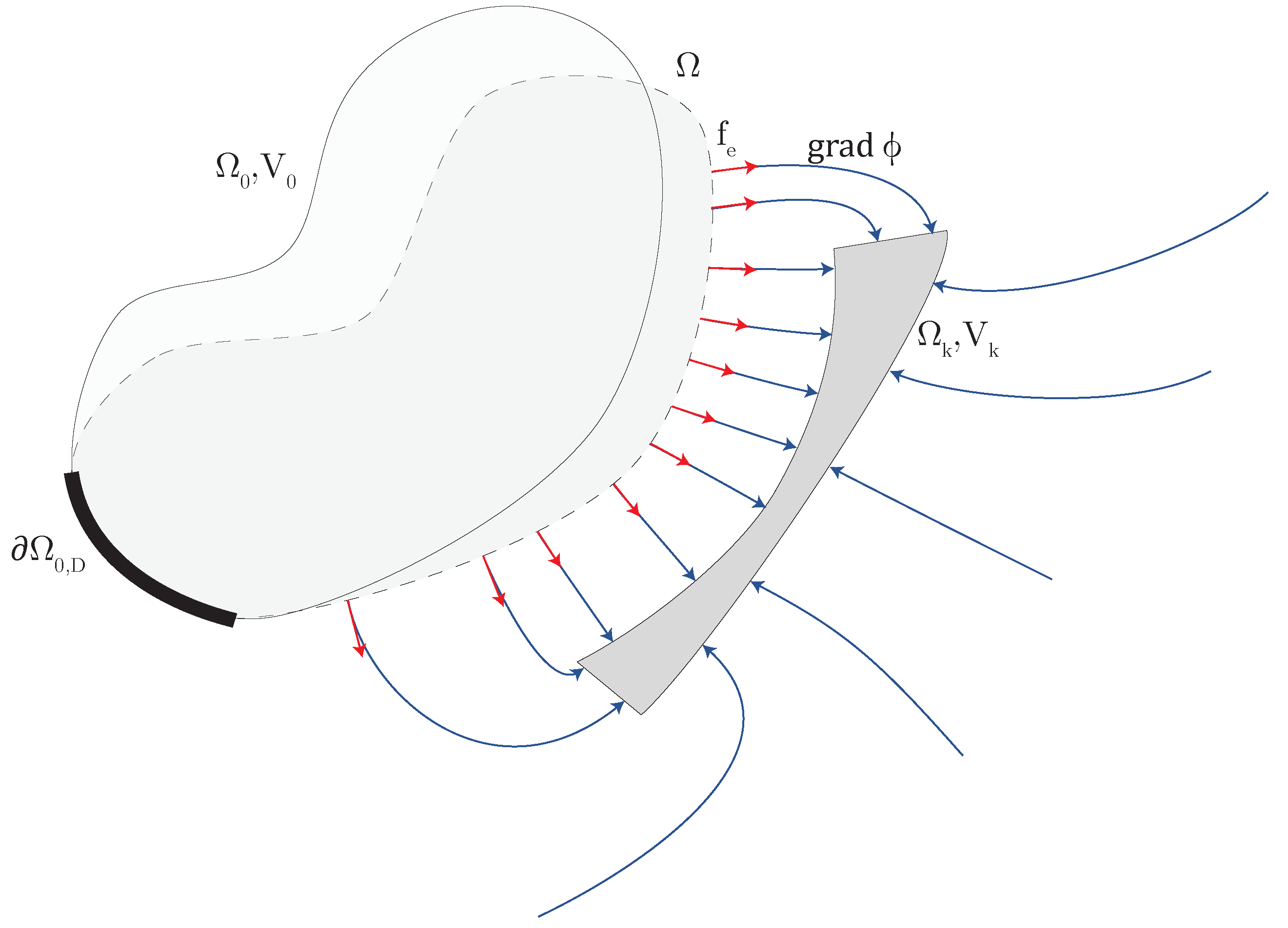
2. Problem Formulation

Let us assume that the device initially occupies the domain ${\Omega }_0$ described by material coordinates $\mathbf{X}$ and is subjected to a transformation $\mathbf{x}=\mathbf{X}+\mathbf{u}(\mathbf{X},t)$, where $\mathbf{u}$ is the displacement vector and $\mathbf{x}$ are the spatial coordinates. Let $\Omega$ denote the current configuration, Figure 1. The boundary in the initial (material) configuration $\partial {\Omega }_0$ is partitioned in $\partial {\Omega }_{0D}$ and $\partial {\Omega }_{0N}$, where Dirichlet and Neumann periodic boundary conditions are enforced, respectively. The Dirichlet boundary conditions are in general time dependent with an angular frequency $\Omega$ and an amplitude ${\tilde{\mathbf{u}}}^D\left(x\right)$. Electrostatic potentials $V_k$ are applied to different portions of the device which is hence subjected to the effects of an electric field. Zero electric flux is assumed on an infinitely distant surface $S_{\infty }$.

Neglecting body forces, the corresponding system of PDEs enforcing periodicity reads:

$$\begin{array}{cc}\hfill {\rho }_0\ddot{\mathbf{u}}(\mathbf{X},t)-\nabla ·\mathbf{P}(\mathbf{X},t)=0& \mathrm{for}(\mathbf{X},t)\mathrm{in}{\Omega }_0\times [0,T],\hfill \end{array}$$

(1)

$$\begin{array}{cc}\hfill \mathbf{P}(\mathbf{X},t)·\mathbf{N}\left(\mathbf{X}\right)={\tilde{\mathbf{f}}}_e& \mathrm{for}(\mathbf{X},t)\mathrm{in}\partial {\Omega }_{0N}\times [0,T],\hfill \end{array}$$

(2)

$$\begin{array}{cc}\hfill \mathbf{u}(\mathbf{X},t)={\tilde{\mathbf{u}}}^D(\mathbf{X},t;\mathit{\mu })& \mathrm{for}(\mathbf{X},t)\mathrm{in}\partial {\Omega }_{0D}\times [0,T],\hfill \end{array}$$

(3)

$$\begin{array}{cc}\hfill \mathbf{u}(\mathbf{X},0)=\mathbf{u}(\mathbf{X},T)& \mathrm{for}\mathbf{X}\mathrm{in}{\Omega }_0,\hfill \end{array}$$

(4)

$$\begin{array}{cc}\hfill \dot{\mathbf{u}}(\mathbf{X},0)=\dot{\mathbf{u}}(\mathbf{X},T)& \mathrm{for}\mathbf{X}\mathrm{in}{\Omega }_0,\hfill \end{array}$$

(5)

$$\begin{array}{cc}\hfill \mathrm{div}\left(\mathrm{grad}\varphi \left(\mathbf{x}\right)\right)=0& \mathrm{in}{\Omega }_{\infty }-\Omega ,\hfill \end{array}$$

(6)

$$\begin{array}{cc}\hfill \varphi \left(\mathbf{x}\right)=V_k& \mathrm{on}\partial {\Omega }_k,\hfill \end{array}$$

(7)

$$\begin{array}{cc}\hfill \mathrm{grad}\varphi \left(\mathbf{x}\right)·\mathbf{n}=0& \mathrm{on}{S}_{\infty }.\hfill \end{array}$$

(8)

Equation (1) expresses the conservation of momentum. ${\rho }_0$ is the initial density, $\mathbf{P}$ is the first Piola–Kirchhoff stress [42], $\mathbf{N}$ and $\mathbf{n}$ denote the normal vectors to the device surface in material and current configurations, respectively, and $\mathit{\varphi }$ is the electrostatic potential scalar field. Here, the gradient operator grad refers to the current configuration $\mathbf{x}$. Equations (2) and (3) are the Neumann and Dirichlet boundary conditions, respectively, with ${\tilde{\mathbf{u}}}^D$ being time periodic. Equations (4) and (5) enforce the periodicity condition on displacements and velocities. The electrostatic pressure ${\mathbf{f}}_e$ on the conductor surface is:

$${\mathbf{f}}_e=\frac{1}{2{ϵ}_0}{\left({ϵ}_0\frac{\partial \mathit{\varphi }\left(\mathbf{x}\right)}{\partial n}\right)}^2\mathbf{n}.$$

(9)

where ${\tilde{\mathbf{f}}}_e$ represents the same force pulled back to the reference configuration.

MEMS devices are usually made of cubic single crystal silicon or polysilicon, thus admitting only small strains, a condition which is well described by the Saint Venant–Kirchhoff constitutive model:

$$\begin{array}{cc}\hfill \mathbf{S}(\mathbf{X},t)=\mathcal{A}\left(\mathbf{X}\right):\mathbf{E}(\mathbf{X},t)& \mathrm{for}(\mathbf{X},t)\mathrm{in}{\Omega }_0\times [0,T],\hfill \end{array}$$

(10)

where $\mathbf{S}$ is the second Piola–Kirchhoff stress, $\mathbf{P}(\mathbf{X},t)=(\mathbf{I}+\nabla \mathbf{u}(\mathbf{X},t\left)\right)·\mathbf{S}(\mathbf{X},t)$, $\mathbf{E}$ is the Green–Lagrange strain tensor, $\mathbf{E}=\frac{1}{2}\left(\nabla \mathbf{u}(\mathbf{X},t)+{\nabla }^T\mathbf{u}(\mathbf{X},t)\right.\left.+{\nabla }^T\mathbf{u}(\mathbf{X},t)·\nabla \mathbf{u}(\mathbf{X},t)\right)$ and $\mathcal{A}$ is the fourth-order elasticity tensor endowed with major and minor symmetries. It is worth stressing that while mechanical equilibrium is naturally formulated in the material coordinates, the electrostatic problem is set in the spatial framework. This additional complexity represents a formidable challenge for modelling approaches like the DPIM which indeed has not been extended to electromechanical problems yet.

3. POD-DL-ROM Technique: Outline and Critical Issues

Here, we briefly review the construction of the deep learning-based ROM (DL-ROM) technique and its extension to the POD-enhanced version (POD-DL-ROM), referring to general time-dependent problems. Later, we will detail why this method is suboptimal for parametrised periodic problems.

The DL-ROM technique is efficient in modelling highly nonlinear time-dependent problems through the identification of the solution manifold underlying the dynamics of the system. This procedure is performed in a non-intrusive, data-driven, black box fashion.

Denoting $\mathit{\mu }\in {\mathbb{R}}^{n_{\mu }}$ as the set of input parameters and $\mathbf{U}\in {\mathbb{R}}^{N_h}$ as the full order model field to be approximated, DL-ROMs aim at approximating the map $(t,\mathit{\mu })\to \mathbf{U}(t,\mathit{\mu })$ by describing both the trial manifold that embeds the transformations between the full order space and the reduced one and the reduced dynamics through deep neural networks.

The method is articulated in three stages. The first one is the encoding stage, in which the encoder function ${\mathbf{f}}_n^E$ maps the full order model (FOM) solutions in a low-dimensional space representation, i.e., latent coordinates ${\tilde{\mathbf{z}}}_n\in {\mathbb{R}}^n$. This is executed through a convolutional autoencoder (CAE). The transformation is formalised as follows:

$${\tilde{\mathbf{z}}}_n(t;\mathit{\mu },{\mathit{\theta }}_E)={\mathbf{f}}_n^E(\mathbf{U}(t;\mathit{\mu });{\mathit{\theta }}_E),$$

(11)

where ${\mathbf{f}}_n^E(·;{\mathit{\theta }}_E):{\mathbb{R}}^{N_h}\to {\mathbb{R}}^n$ and ${\mathit{\theta }}_E$ is the parameter vector of the CAE. The second stage is reduced dynamics learning, which aims at describing the dynamical evolution of the intrinsic (latent) coordinates of the ROM approximation. The corresponding function modelled is:

$${\mathbf{z}}_n(t;\mathit{\mu },{\mathit{\theta }}_{DF})={\mathsf{\varphi }}_n^{DF}(t;\mathit{\mu },{\mathit{\theta }}_{DF}),$$

(12)

where ${\mathit{\varphi }}_n^{DF}(·;·,{\mathit{\theta }}_{DF}):{\mathbb{R}}^{(n_{\mathit{\mu }}+1)}\to {\mathbb{R}}^n$. In the standard DL-ROM method, reduced dynamics learning is performed through a deep feedforward neural network with parameters ${\mathit{\theta }}_{DF}$. The third and final stage is the decoding stage, where the latent coordinates are mapped back to the full order model space:

$$\begin{array}{c}\hfill {\tilde{\mathcal{S}}}_h^n=\{{\mathbf{f}}_h^D({\mathbf{z}}_n(t;\mathit{\mu },{\mathit{\theta }}_{DF});{\mathit{\theta }}_D):{\mathbf{z}}_n(t;\mathit{\mu },{\mathit{\theta }}_{DF})\in {\mathbb{R}}^n,t\in [0,T),\mathit{\mu }\in {\mathbb{R}}^{n_{\mathit{\mu }}}\}\subset {\mathbb{R}}^{N_h},\end{array}$$

(13)

where ${\tilde{\mathcal{S}}}_h^n$ is the approximation of the full order solution manifold, and ${\mathbf{f}}^D(·;{\mathit{\theta }}_D):{\mathbb{R}}^n\to {\mathbb{R}}^{N_h}$ depends upon a vector ${\mathit{\theta }}_D$ collecting all the corresponding weights and biases. Furthermore, in this case, we employ a CAE to represent this function [43,44]. During the training stage, two loss functions $\mathcal{L}$ have to be enforced:

$$\begin{array}{c}\hfill {\mathcal{L}}_1=\frac{{\omega }_h}{2}\left|\right|{\mathbf{f}}_h^D\left({\mathbf{z}}_n\right)-\mathbf{U}{\left|\right|}^2\\ \hfill {\mathcal{L}}_2=\frac{1-{\omega }_h}{2}\left|\right|{\mathbf{f}}_n^E\left(\mathbf{U}\right)-{\mathbf{z}}_n{\left|\right|}^2\end{array}$$

(14)

with the ${\omega }_h$ parameter tuning the relative importance of the two losses.

The DL-ROM approximation in the testing stage $\tilde{\mathbf{U}}(t;\mathit{\mu })\approx \mathbf{U}(t;\mathit{\mu })$ involves only reduced dynamics learning and decoding stage functions, and is then given by

$$\tilde{\mathbf{U}}(t;\mathit{\mu },{\mathit{\theta }}_{DF},{\mathit{\theta }}_D)={\mathbf{f}}_h^D({\mathit{\varphi }}_n^{DF}(t;\mathit{\mu },{\mathit{\theta }}_{DF});{\mathit{\theta }}_D).$$

(15)

Further details are available in [33].

This approach is quite general; nevertheless, training the neural network with a set of coordinates as large as the original FOM system leads easily to a computational burden not manageable with standard computing facilities. These issues are partially solved by the POD-DL-ROM variant of the DL-ROM method. The corresponding architecture is depicted in Figure 2. In particular, POD is initially applied to the snapshot set using randomised SVD (rSVD), which reduces the dimensionality of the snapshots. Next, a DL-ROM is constructed to represent the map between $(t,\mathit{\mu })$ and the POD-generalised coordinates ${\mathbf{u}}_N(t;\mathit{\mu })={\mathbf{V}}_N^T\mathbf{U}(t;\mathit{\mu })\in {\mathbb{R}}^N$, with ${\mathbf{V}}_N^T$ proper orthogonal modes computed by the rSVD. Referring to the DL-ROM stages detailed previously, this basically adds the application of a linear transformation onto the linear trial manifold defined by ${\mathbf{V}}_N$ to the encoding and decoding stages. The input of the encoder and the output of the decoder functions will have dimension N instead of $N_h$, while no relevant changes are applied to the reduced dynamics learning stages.

Despite the generality of POD-DL-ROM [33,34,36,45,46], some difficulties arise when tackling parameterised periodic problems. In particular, when modelling periodic solutions, the standard POD-DL-ROM approach would require the parametrisation of the dynamic behaviour directly with respect to the time variable. This means that one should generate enough snapshots to describe the time evolution over the period up to the desired resolution, and this has to be done for each parameter value to guarantee a proper generalisation. This procedure is quite inefficient for two reasons: (1) the amount of data to be processed by the neural network grows with the number of snapshots retained along the period, which is critical as their number and distribution highly influence the time response quality of the solution and (2) it requires more parameters to be trained since the time dependency must be explicitly modelled. This is not optimal for a periodic problem where the underlying dynamics are inherently simple and time invariant. This work addresses these issues by exploiting the a priori knowledge of the periodic behaviour of the data in the pre-processing stage of the POD-DL-ROM approach. This is achieved by resorting to a harmonic decomposition of the periodic time series feeding the POD-DL-ROM method, thus removing the time variable dependence in the modelling with a strong reduction in the number of snapshots to be provided and consequently a reduction in the number of parameters to be trained in the neural networks.

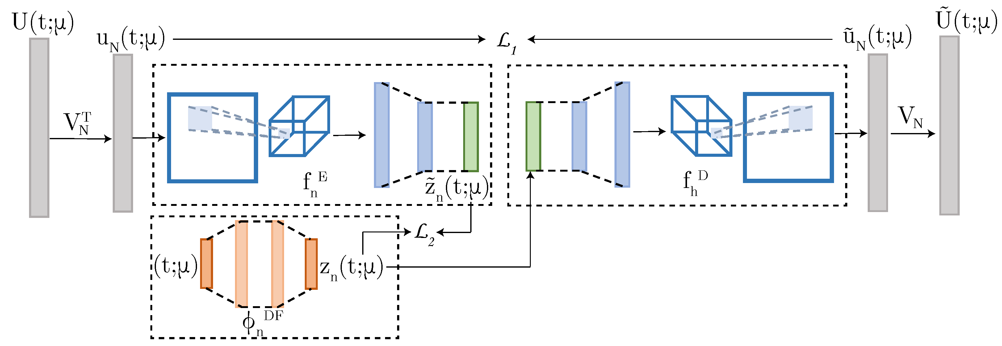
4. Periodic DL-ROM Technique

The proposed method, i.e., Periodic POD-enhanced deep learning-based ROM (Periodic POD-DL-ROM or Periodic DL-ROM for short), is composed of the same main stages as the standard POD-DL-ROM with additional pre-processing and post-processing steps. The reduced dynamics learning will now be named periodicity pattern learning.

The encoding stage includes three separate encoding functions: POD linear subspace projection, harmonic decomposition, and nonlinear encoding towards the latent coordinate manifold. The harmonic decomposition function $\mathcal{H}$ aims at removing the time dependence from the periodic signal. This is possible if the period $T\left(\mathit{\mu }\right)$ of the time series can be determined with some data pre-treatment, e.g., a fast Fourier transform.

Given a training set of FOM solutions projected onto the linear POD subspace ${\mathrm{u}}_N^j(t;\mathit{\mu })$ with $j=1,..,N$, these can be approximated by expanding the system state as a Fourier series with angular frequency $\omega =2\pi /T$, truncated up to the desired order K:

$${\mathrm{u}}_N^j(t;\mathit{\mu })\approx \mathcal{H}(t;\omega ,a_k\left(\mathit{\mu }\right),b_k\left(\mathit{\mu }\right))=\frac{a_0^j}{2}+\sum _{k=1}^K{a}_k^j\cos \left(k\omega t\right)+b_k^j\sin \left(k\omega t\right),$$

(16)

where $a_k^j\in \mathbb{R}$ and $b_k^j\in \mathbb{R}$ are the coefficients multiplying the k-th harmonics of the Fourier series approximation of the j-th coordinate. An order K approximation leads to $N_F=2K+1$ coefficients. These coefficients for each POD coordinate are collected in a matrix ${\mathbf{c}}_N\left(\mathit{\mu }\right)$. These harmonic coefficients depend on the parameter values $\mathit{\mu }$. The new specialised encoding stage is formalised as follows:

$${\tilde{\mathbf{z}}}_n(\mathit{\mu },{\mathit{\theta }}_E)={\mathbf{f}}_n^E({\mathcal{H}}^{-1}\left({\mathbf{V}}_N^T\mathbf{U}(t;\mathit{\mu })\right);{\mathit{\theta }}_E)={\mathbf{f}}_n^E({\mathbf{c}}_N\left(\mathit{\mu }\right);{\mathit{\theta }}_E);$$

(17)

The second stage, now named periodicity pattern learning, aims at describing the reduced latent representation of the evolution of the harmonic coefficients. This is modelled by means of interpolation methods using, e.g., piecewise linear functions or splines, and generates a function $\mathcal{I}$ such that:

$${\mathbf{z}}_n\left(\mathit{\mu }\right)=\mathcal{I}\left(\mathit{\mu }\right)$$

(18)

The decoding stage is consequently expressed as:

$${\tilde{\mathbf{c}}}_N\left(\mathit{\mu }\right)={\mathbf{f}}_h^D({\mathbf{z}}_n\left(\mathit{\mu }\right);{\mathit{\theta }}_D)$$

(19)

where ${\tilde{\mathbf{c}}}_N\left(\mathit{\mu }\right)$ is an approximation of the harmonic coefficient matrix provided to the system. The Periodic POD-DL-ROM approximation in the testing stage is then given by:

$$\tilde{\mathbf{U}}(t;\mathit{\mu },{\mathit{\theta }}_D)={\mathbf{V}}_N\mathcal{H}(t;\omega ,{\mathbf{f}}_h^D(\mathcal{I}\left(\mathit{\mu }\right);{\mathit{\theta }}_D))$$

(20)

During the training stage, only one loss function ${\mathcal{L}}_1$ has to be minimised and it is based on the harmonic coefficients matrices:

$$\begin{array}{c}\hfill {\mathcal{L}}_1=\left|\right|{\mathbf{f}}_h^D\left({\tilde{\mathbf{z}}}_n\right)-{\mathbf{c}}_N{\left|\right|}^2\end{array}$$

(21)

Even though the procedure highlighted here is very similar to the standard POD-DL-ROM, one should nevertheless also consider that the harmonic decomposition (and its inverse) requires knowing the period of the system response, which may be given as an input parameter or, as detailed in the following, treated as another target value to be modelled with respect to the input parameters. This feature does not significantly change the stages of the Periodic DL-ROM approach; it will only need additional tools to parametrise the period along with the system response. The Periodic DL-ROM procedure is schematically represented in Figure 3.

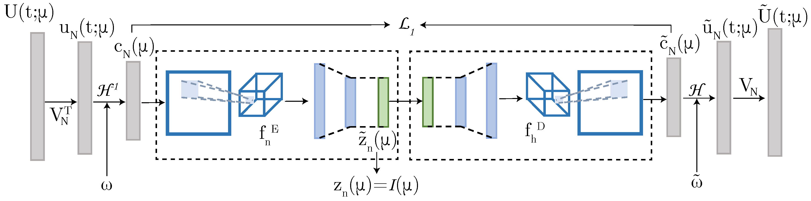
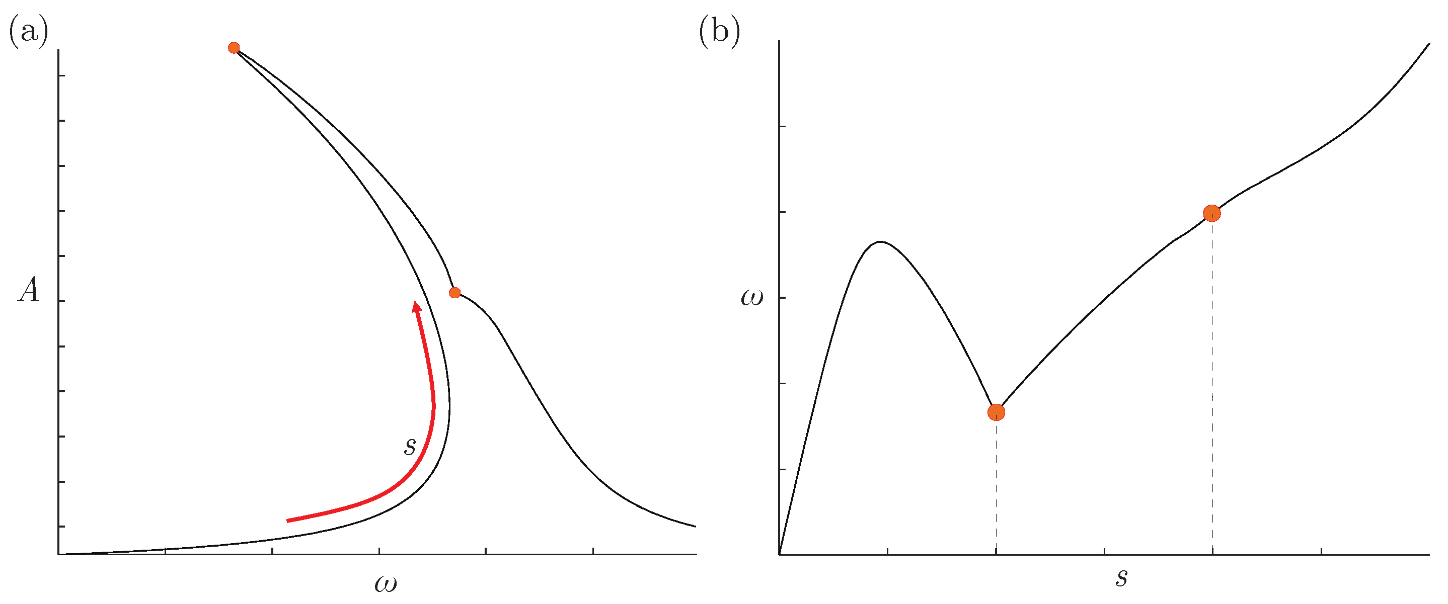
5. Frequency Response Function Modelling: Arch Length Abscissa

In MEMS simulations and experimental analyses, one of the most commonly used outputs is the frequency response curve (FRC), which defines the steady-state periodic response of the dynamical system, i.e., the collection of periodic solutions (stable and unstable) along a given branch. The FRC represents the outcomes of the device’s behaviour as a function of the actuation intensity and frequency. In nonlinear systems, like those emerging from the electromechanical modelling of MEMSs, the FRC is not a single-valued function of the forcing frequency $\omega$, see Figure 4a. To overcome these difficulties, a possible solution is given by the approach proposed in [37], where instead of using the actuation frequency as an input parameter, this is replaced by a curvilinear abscissa that directly parametrises the FRC of interest. This additionally requires a model for the frequency value with respect to the other input parameters and the abscissa itself, see Figure 4b. In general, this model is nonlinear and can be represented in different ways. Here, we resort to a simple interpolation method.

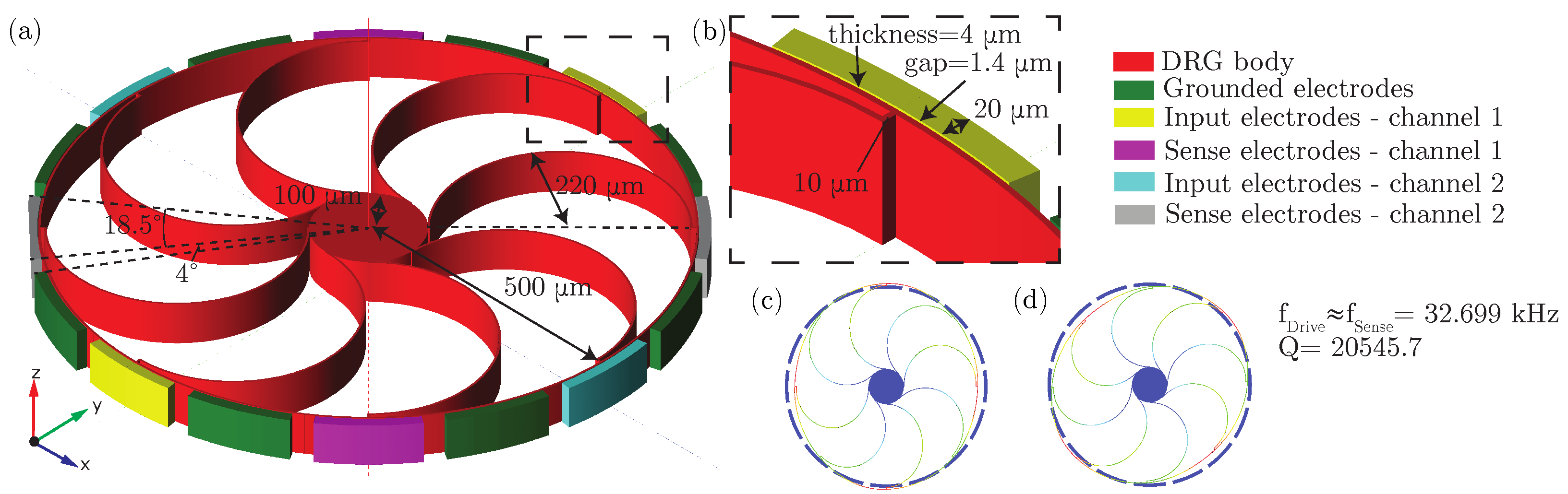
6. Application: Electromechanical Disk Resonating Gyroscope

In this section, as an example with industrial relevance, we will address a disk resonating gyroscope (DRG) inspired by the device proposed in [47]. The DRG is modelled with the software Coventor MEMS+^TM 7.1 using one of the templates available in the software itself, slightly modified for the purposes of this work [48,49,50].

6.1. Problem Description

In Figure 5a,b, the gyroscope geometry is reported, and its components are coloured according to their function.

Euler–Bernulli beam elements are used to discretise the arch suspensions (two elements each) and the external ring of the DRG (32 elements). A stiff cylinder, restrained to the ground, serves as a central support. The ring is surrounded by a sequence of parallel plate electrodes, and the software uses conformal mappings to describe the electrostatic forces. We emphasise that the predicted displacements are minimal with respect to the element size, allowing us to ignore geometric nonlinearities as all nonlinear effects are induced by the electromechanical interaction.

In particular, the DRG has the two degenerate modes shown in Figure 5c,d, which are characterised by radial displacements of the outer ring proportional to $cos\left(2\mathit{\theta }\right)$ and $sin\left(2\mathit{\theta }\right)$, with the $\mathit{\theta }$ polar coordinate running on the external ring. This device is designed to sense angular velocities around the Z axis. Indeed, if the former (drive) mode is actuated, the Coriolis effect also activates the latter mode, which can be sensed [47]. However, for certain operating conditions, the coupling between the modes gets stronger and the device displays an autoparametric resonance between the drive and the sense mode. Indeed, the drive mode modulates the stiffness of the sense one at a frequency of $2f_{\mathrm{drive}}$ and this triggers the parametric resonance.

The drive mode in Figure 5c is activated during operations by applying the bias $V_{\mathrm{AC}}sin\omega t$ to the blue electrodes and the bias $-V_{\mathrm{AC}}sin\omega t$ to the yellow electrodes. A constant potential bias of $V_{\mathrm{DC}}=1$ V is imposed on the gyro (red structure). All the remaining electrodes are grounded.

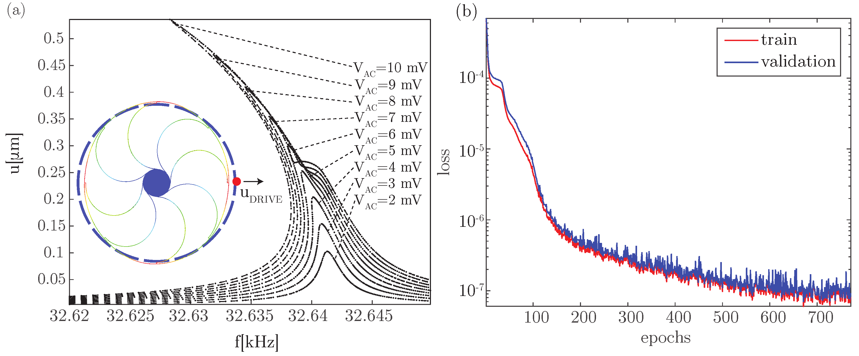
6.2. Hyperparameters and Training

The collected dataset used during the training process is given by 1797 combinations of frequency and external excitation amplitudes distributed on the FRC. The number of POD bases retained is 11, and the harmonic decomposition is truncated at order 9. The training parameter space spans $f=[32.620,32.6498]$ kHz, $V_{\mathrm{AC}}=[2,3,4,5,6,7,8,9,10]$ mV, and the sampling points are reported in Figure 6a. The neural network was trained with AdaMAX and an early stopping algorithm setting the maximum number of epochs to 5000. The collected dataset was randomly split into a training and validation set with a 0.7 ratio, see Figure 6b. The batch size is 16. In this application, the latent space dimension n was fixed at 4. Choosing an appropriate latent size is essential. The minimum latent size is influenced by the number of input parameters and the dynamic features of the problem. Since the system displays modal interaction between two modes, the minimum size is 2, but to ensure the quality of the problem, a higher dimensional space is advised, see [37]. The framework used for this implementation was the Julia library Flux [51]. Details concerning the convolutional autoencoder are reported in

Table 1. Features of convolutional and dense layers in the encoder ${\mathbf{f}}_n^E$. The total number of parameters is 6651. The stride was always set to one and a padding equal to zero was used. There are two input channels because the FOM deploys Euler–Bernulli beams, so displacements and rotations DOFs are kept separated. The encoding process reduces the input matrix with a shape of $N,N_F,2$ towards a bottleneck representation with a size n, with N number of POMs, $N_F$ number of harmonic terms, and n latent dimensions.

Layer	Input	Output	Kernel	# of Filters
	Dimension	Dimension	Size
1	[N, $N_F$, 2]	[$N-1$, $N_F-1$, 3]	[2, 2]	3
2	[$N-1$, $N_F-1$, 3]	[$N-2$, $N_F-2$, 5]	[5, 5]	5
3	[$N-2$, $N_F-2$, 5]	[$N-3$, $N_F-3$, 5]	[5, 5]	5
5	$(N-3)(N_F-3)5$	10
6	10	n

and

Table 2. Features of dense and transposed convolutional layers in the decoder ${\mathbf{f}}_N^D$. The total number of parameters is 7284. The stride was always set to one and a padding equal to zero was used. There are two input channels because the FOM utilises Euler–Bernulli beams with both displacements and rotations DOFs. The decoding process expands the latent representation matrix with a size n towards a matrix with a shape $N,N_F,2$, with N number of POMs, $N_F$ number of harmonic terms, and n latent dimensions.

Layer	Input	Output	Kernel	# of Filters
	Dimension	Dimension	Size
1	n	10
2	10	$(N-3)(N_F-3)5$
3	[$N-3$, $N_F-3$, 5]	[$N-2$, $N_F-2$, 5]	[2, 2]	5
4	[$N-2$, $N_F-2$, 5]	[$N-1$, $N_F-1$, 3]	[2, 2]	3
5	[$N-1$, $N_F-1$, 3]	[N, $N_F$, 2]	[2, 2]	2

. Motivated by the fact that the number of parameters to be trained is kept low and the proposed architecture is particularly robust since it stems from the well-established POD-DL-ROM framework, the hyperparameter tuning procedure is performed by trial and error experiments. A detailed description of this procedure can be found in previous publications, e.g., [34].

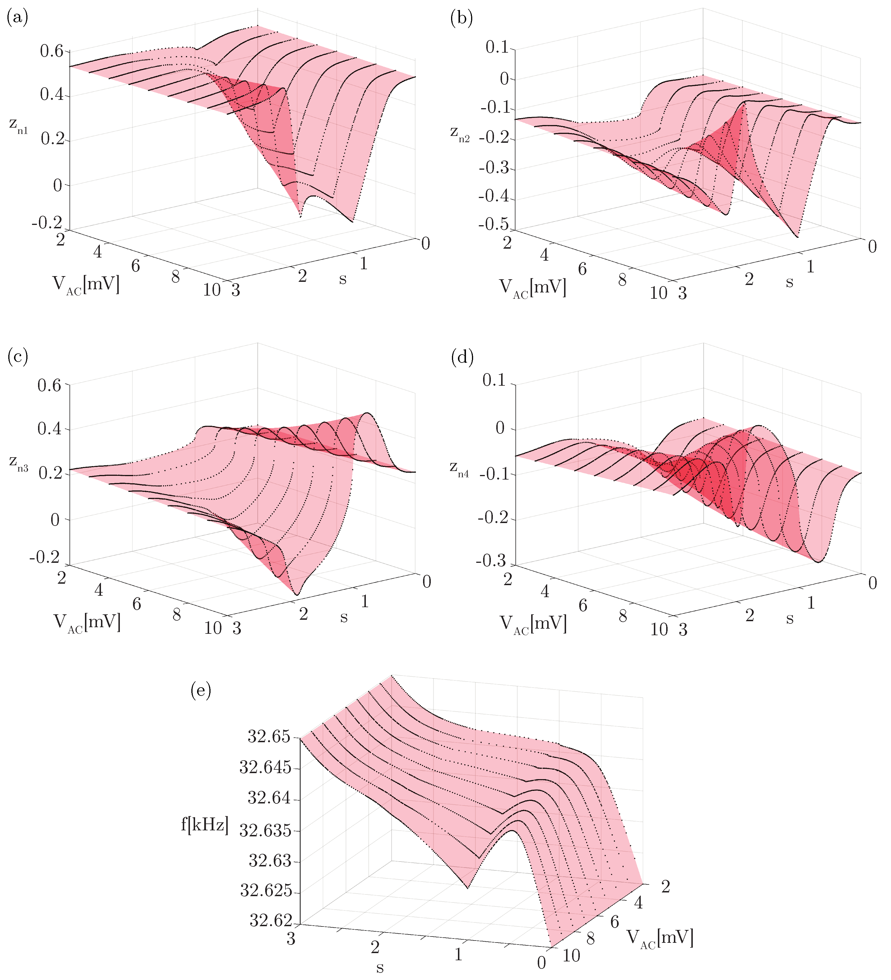
6.3. Latent Coordinates and Frequency Features

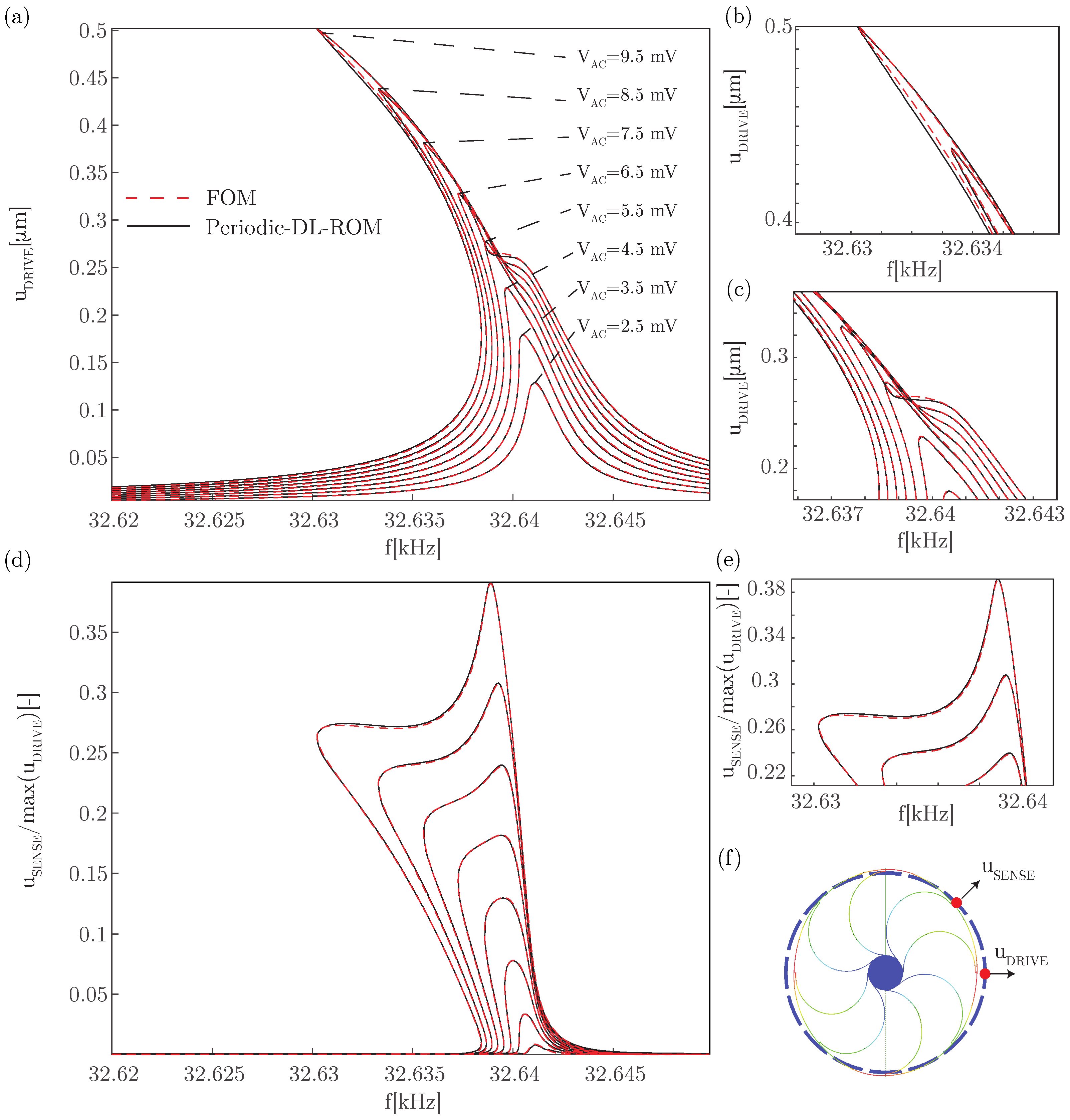
After the convolutional autoencoder training stage, the resulting latent coordinates, as well as the frequency, are modelled with spline interpolation functions. The latent coordinates and angular frequency are plotted in Figure 7a–e versus the parameters of the problem at hand, i.e., s and $V_{AC}$. The resulting surfaces are smooth with local discontinuity at the switching point between different abscissa intervals, i.e., $s=1,2$. Such a behaviour is expected and is a consequence of the arc length abscissa approach used to uniquely define the relationship with respect to the amplitude and the frequency. The limit points of different abscissa regions are such that they align with important features, e.g., peak response and resonances. These lead to regions with different sizes and, consequently, a local discontinuity between the regions modelled.

6.4. Results

The reconstruction of the displacement field of the DRG with the Periodic DL-ROM allows building the FRCs in Figure 8 related to testing $V_{AC}$ values only. The testing instances considered here are inside the training parameter space and refer to points representative of the drive and sense modes of the DRG, respectively, highlighted with red dots in Figure 8f. The Periodic DL-ROM solution is able to accurately reproduce most of the FRCs features and shows good agreement with the reference FOM. Some differences can be observed close to the peaks of the drive motion on the highest forcing levels, see Figure 8b. These curves represent the most critical ones because they are close to the boundaries of the parameter space, and thus fewer data points characterise that region’s neighborhood. Nevertheless, the error given by the Periodic DL-ROM is negligible. The plateau region at the highest forcing values, i.e., $V_{AC}$ > 7.5 mV, corresponds to the auto-parametric resonance effect between the drive and the sense modes. Here, the Periodic DL-ROM well reproduces the overall shape with minor differences with respect to the FOM solution (Figure 8c). Similar remarks hold also for the FRCs of the sense motion (Figure 8d,e).

6.5. Key Advantages and Comparison with POD-DL-ROM

The Periodic DL-ROM can reproduce complex dynamics like those presented in this section in almost real time, a capability shared with the POD-DL-ROM from which our approach stems. To better highlight the advantages of our proposal with respect to the POD-DL-ROM, let us consider data taken from the example at hand. Here, the neural network has 13,935 parameters which is significantly less than the 360,000 parameters utilised by the POD-DL-ROM in a similar problem [36]. This tremendous reduction, which is achieved thanks to the harmonic decomposition, sets much less stringent requirements on the computational resources. Indeed, the Periodic DL-ROM can be trained in a few minutes on a standard CPU instead of hours on a high-end GPU [37]. Once trained, the performance of Periodic DL-ROM is almost in real time. For example, the generation of all the 4660 instances collected in Figure 8 takes less than 10 s on a standard workstation with an AMD Ryzen 9 5950X CPU. Hence, the time per instance is approximately 2 milliseconds, also including the reconstruction of 100 time snapshots over one period starting from the Fourier coefficients provided by the decoder.

Finally, it is worth stressing that the Periodic DL-ROM, as well as the POD-DL-ROM, can accurately reproduce any field of interest everywhere in the device, e.g., displacements and stresses [37], that is accessible through the original FOM. All the features listed here are desirable in many problems and applications ranging from online control to design optimisation.

7. Conclusions

In this work, we have proposed an alternative algorithm stemming from the POD-DL-ROM method able to tackle periodic problems in MEMS applications in an effective way. Starting from simple assumptions about the full order data available, the theoretical setup of the method has been explained and compared with previous techniques. Then, the effectiveness of the procedure was verified on a coupled electromechanical problem, i.e., a disk resonating gyroscope. The proposed method is able to match the performance of the POD-DL-ROM method while allowing a strong reduction in terms of the number of parameters of the neural network to be trained and, correspondingly, a reduction in the computational effort required. Furthermore, the injection of prior knowledge about the periodicity of the solution into the neural network allows us to enforce it automatically through a data pre-processing phase.

References

1. Vizzaccaro, A.; Givois, A.; Longobardi, P.; Shen, Y.; Deü, J.F.; Salles, L.; Touzé, C.; Thomas, O. Non-intrusive reduced order modelling for the dynamics of geometrically nonlinear flat structures using three-dimensional finite elements. Comput. Mech. 2020, 66, 1293–1319. [Google Scholar] [CrossRef]
2. Touzé, C.; Vizzaccaro, A.; Thomas, O. Model order reduction methods for geometrically nonlinear structures: A review of nonlinear techniques. Nonlinear Dyn. 2021, 105, 1141–1190. [Google Scholar] [CrossRef]
3. Kerschen, G.; Golinval, J.C.; Vakakis, A.F.; Bergman, L.A. The method of proper orthogonal decomposition for dynamical characterization and order reduction of mechanical systems: An overview. Nonlinear Dyn. 2005, 41, 147–169. [Google Scholar] [CrossRef]
4. Amabili, M.; Touzé, C. Reduced-order models for nonlinear vibrations of fluid-filled circular cylindrical shells: Comparison of POD and asymptotic nonlinear normal modes methods. J. Fluids Struct. 2007, 23, 885–903. [Google Scholar] [CrossRef] [Green Version]
5. Amabili, M.; Sarkar, A.; Paıdoussis, M. Reduced-order models for nonlinear vibrations of cylindrical shells via the proper orthogonal decomposition method. J. Fluids Struct. 2003, 18, 227–250. [Google Scholar] [CrossRef]
6. Gobat, G.; Opreni, A.; Fresca, S.; Manzoni, A.; Frangi, A. Reduced order modeling of nonlinear microstructures through Proper Orthogonal Decomposition. Mech. Syst. Signal Process. 2022, 171, 108864. [Google Scholar] [CrossRef]
7. Frangi, A.; Gobat, G. Reduced order modelling of the non-linear stiffness in MEMS resonators. Int. J. -Non-Linear Mech. 2019, 116, 211–218. [Google Scholar] [CrossRef]
8. Zega, V.; Gobat, G.; Fedeli, P.; Carulli, P.; Frangi, A.A. Reduced Order Modelling in a Mems Arch Resonator Exhibiting 1: 2 Internal Resonance. In Proceedings of the 2022 IEEE 35th International Conference on Micro Electro Mechanical Systems Conference (MEMS), Tokyo, Japan, 9–13 January 2022; IEEE: Piscataway Township, NJ, USA; pp. 499–502. [Google Scholar]
9. Gobat, G.; Zega, V.; Fedeli, P.; Guerinoni, L.; Touzé, C.; Frangi, A. Reduced order modelling and experimental validation of a MEMS gyroscope test-structure exhibiting 1: 2 internal resonance. Sci. Rep. 2021, 11, 16390. [Google Scholar] [CrossRef]
10. Gobat, G.; Guillot, L.; Frangi, A.; Cochelin, B.; Touzé, C. Backbone curves, Neimark-Sacker boundaries and appearance of quasi-periodicity in nonlinear oscillators: Application to 1: 2 internal resonance and frequency combs in MEMS. Meccanica 2021, 56, 1937–1969. [Google Scholar] [CrossRef]
11. Mahdiabadi, M.K.; Tiso, P.; Brandt, A.; Rixen, D.J. A non-intrusive model-order reduction of geometrically nonlinear structural dynamics using modal derivatives. Mech. Syst. Signal Process. 2021, 147, 107126. [Google Scholar] [CrossRef]
12. Wu, L.; Tiso, P. Nonlinear model order reduction for flexible multibody dynamics: A modal derivatives approach. Multibody Syst. Dyn. 2016, 36, 405–425. [Google Scholar] [CrossRef] [Green Version]
13. Vizzaccaro, A.; Salles, L.; Touzé, C. Comparison of nonlinear mappings for reduced-order modelling of vibrating structures: Normal form theory and quadratic manifold method with modal derivatives. Nonlinear Dyn. 2021, 103, 3335–3370. [Google Scholar] [CrossRef]
14. Shaw, S.; Pierre, C. Non-linear normal modes and invariant manifolds. J. Sound Vib. 1991, 150, 170–173. [Google Scholar] [CrossRef] [Green Version]
15. Shaw, S.W.; Pierre, C. Normal modes for non-linear vibratory systems. J. Sound Vib. 1993, 164, 85–124. [Google Scholar] [CrossRef] [Green Version]
16. Ponsioen, S.; Pedergnana, T.; Haller, G. Automated computation of autonomous spectral submanifolds for nonlinear modal analysis. J. Sound Vib. 2018, 420, 269–295. [Google Scholar] [CrossRef] [Green Version]
17. Vizzaccaro, A.; Shen, Y.; Salles, L.; Blahoš, J.; Touzé, C. Direct computation of nonlinear mapping via normal form for reduced-order models of finite element nonlinear structures. Comput. Methods Appl. Mech. Eng. 2021, 384, 113957. [Google Scholar] [CrossRef]
18. Opreni, A.; Vizzaccaro, A.; Frangi, A.; Touzé, C. Model Order Reduction based on Direct Normal Form: Application to Large Finite Element MEMS Structures Featuring Internal Resonance. Nonlinear Dyn. 2021, 105, 1237–1272. [Google Scholar] [CrossRef]
19. Vizzaccaro, A.; Opreni, A.; Salles, L.; Frangi, A.; Touzé, C. High order direct parametrisation of invariant manifolds for model order reduction of finite element structures: Application to large amplitude vibrations and uncovering of a folding point. Nonlinear Dyn. 2022, 110, 525–571. [Google Scholar] [CrossRef]
20. Jain, S.; Haller, G. How to compute invariant manifolds and their reduced dynamics in high-dimensional finite element models. Nonlinear Dyn. 2022, 107, 1417–1450. [Google Scholar] [CrossRef]
21. Opreni, A.; Vizzaccaro, A.; Touzé, C.; Frangi, A. High-order direct parametrisation of invariant manifolds for model order reduction of finite element structures: Application to generic forcing terms and parametrically excited systems. Nonlinear Dyn. 2023, 111, 5401–5447. [Google Scholar] [CrossRef]
22. Hesthaven, J.S.; Ubbiali, S. Non-intrusive reduced order modeling of nonlinear problems using neural networks. J. Comput. Phys. 2018, 363, 55–78. [Google Scholar] [CrossRef] [Green Version]
23. San, O.; Maulik, R. Neural network closures for nonlinear model order reduction. Adv. Comput. Math. 2018, 44, 1717–1750. [Google Scholar] [CrossRef] [Green Version]
24. Dutta, S.; Rivera-Casillas, P.; Styles, B.; Farthing, M.W. Reduced order modeling using advection-aware autoencoders. Math. Comput. Appl. 2022, 27, 34. [Google Scholar] [CrossRef]
25. Wang, Q.; Ripamonti, N.; Hesthaven, J.S. Recurrent neural network closure of parametric POD-Galerkin reduced-order models based on the Mori-Zwanzig formalism. J. Comput. Phys. 2020, 410, 109402. [Google Scholar] [CrossRef]
26. Fatone, F.; Fresca, S.; Manzoni, A. Long-time prediction of nonlinear parametrized dynamical systems by deep learning-based reduced order models. arXiv 2022, arXiv:2201.10215. [Google Scholar]
27. Hernández, Q.; Badías, A.; Chinesta, F.; Cueto, E. Thermodynamics-informed graph neural networks. arXiv 2022, arXiv:2203.01874. [Google Scholar] [CrossRef]
28. Nguyen, T.; Li, Z.; Silander, T.; Leong, T.Y. Online feature selection for model-based reinforcement learning. In Proceedings of the International Conference on Machine Learning, Atlanta, GA, USA, 17–19 June 2013; PMLR, 2013; pp. 498–506. [Google Scholar]
29. Cai, S.; Mao, Z.; Wang, Z.; Yin, M.; Karniadakis, G.E. Physics-informed neural networks (PINNs) for fluid mechanics: A review. Acta Mech. Sin. 2021, 37, 1727–1738. [Google Scholar] [CrossRef]
30. Wu, P.; Qiu, F.; Feng, W.; Fang, F.; Pain, C. A non-intrusive reduced order model with transformer neural network and its application. Phys. Fluids 2022, 34, 115130. [Google Scholar] [CrossRef]
31. Sitapure, N.; Kwon, J.S.I. Exploring the potential of time-series transformers for process modeling and control in chemical systems: An inevitable paradigm shift? Chem. Eng. Res. Des. 2023, 194, 461–477. [Google Scholar] [CrossRef]
32. Sitapure, N.; Kwon, J.S. CrystalGPT: Enhancing system-to-system transferability in crystallization prediction and control using time-series-transformers. arXiv 2023, arXiv:2306.03099. [Google Scholar] [CrossRef]
33. Fresca, S.; Dede, L.; Manzoni, A. A comprehensive deep learning-based approach to reduced order modeling of nonlinear time-dependent parametrized PDEs. J. Sci. Comput. 2021, 87, 1–36. [Google Scholar] [CrossRef]
34. Fresca, S.; Manzoni, A. POD-DL-ROM: Enhancing deep learning-based reduced order models for nonlinear parametrized PDEs by proper orthogonal decomposition. Comput. Methods Appl. Mech. Eng. 2022, 388, 114181. [Google Scholar] [CrossRef]
35. Cicci, L.; Fresca, S.; Manzoni, A. Deep-HyROMnet: A Deep Learning-Based Operator Approximation for Hyper-Reduction of Nonlinear Parametrized PDEs. J. Sci. Comput. 2022, 93, 57. [Google Scholar] [CrossRef]
36. Fresca, S.; Gobat, G.; Fedeli, P.; Frangi, A.; Manzoni, A. Deep learning-based reduced order models for the real-time simulation of the nonlinear dynamics of microstructures. Int. J. Numer. Methods Eng. 2022, 123, 4749–4777. [Google Scholar] [CrossRef]
37. Gobat, G.; Fresca, S.; Manzoni, A.; Frangi, A. Reduced Order Modeling of Nonlinear Vibrating Multiphysics Microstructures with Deep Learning-Based Approaches. Sensors 2023, 23, 3001. [Google Scholar] [CrossRef]
38. Yu, J.; Wen, Y.; Yang, L.; Zhao, Z.; Guo, Y.; Guo, X. Monitoring on triboelectric nanogenerator and deep learning method. Nano Energy 2022, 92, 106698. [Google Scholar] [CrossRef]
39. Bangi, M.S.F.; Kwon, J.S.I. Deep reinforcement learning control of hydraulic fracturing. Comput. Chem. Eng. 2021, 154, 107489. [Google Scholar] [CrossRef]
40. Singh Sidhu, H.; Siddhamshetty, P.; Kwon, J.S. Approximate dynamic programming based control of proppant concentration in hydraulic fracturing. Mathematics 2018, 6, 132. [Google Scholar] [CrossRef] [Green Version]
41. Lee, J.H.; Wong, W. Approximate dynamic programming approach for process control. J. Process. Control 2010, 20, 1038–1048. [Google Scholar] [CrossRef]
42. Malvern, L. Introduction to the Mechanics of a Continuous Medium; Prentice-Hall Series in Engineering of the Physical Sciences; Prentice-Hall: Englewood Cliffs, NJ, USA, 1969. [Google Scholar]
43. LeCun, Y.; Bottou, L.; Bengio, Y.; Haffner, P. Gradient-based learning applied to document recognition. Proc. IEEE 1998, 86, 2278–2324. [Google Scholar] [CrossRef]
44. Hinton, G.E.; Zemel, R. Autoencoders, minimum description length and Helmholtz free energy. Adv. Neural Inf. Process. Syst. 1993, 6, 3–10. [Google Scholar]
45. Fresca, S.; Manzoni, A.; Dedè, L.; Quarteroni, A. Deep learning-based reduced order models in cardiac electrophysiology. PLoS ONE 2020, 15, e0239416. [Google Scholar] [CrossRef]
46. Fresca, S.; Manzoni, A. Real-time simulation of parameter-dependent fluid flows through deep learning-based reduced order models. Fluids 2021, 6, 259. [Google Scholar] [CrossRef]
47. Ayazi, F.; Najafi, K. A HARPSS polysilicon vibrating ring gyroscope. J. Microelectromech. Syst. 2001, 10, 169–179. [Google Scholar] [CrossRef] [Green Version]
48. Coventor Inc., A Lam Research Company. Coventor MEMS+TM. Available online: https://www.coventor.com/ (accessed on 1 March 2023).
49. Parent, A.; Krust, A.; Lorenz, G.; Favorskiy, I.; Piirainen, T. Efficient nonlinear simulink models of MEMS gyroscopes generated with a novel model order reduction method. In Proceedings of the 2015 Transducers-2015 18th International Conference on Solid-State Sensors, Actuators and Microsystems (TRANSDUCERS), Anchorage, Alaska, 21–25 June 2015; IEEE: Piscataway Township, NJ, USA, 2015; pp. 2184–2187. [Google Scholar]
50. Parent, A.; Krust, A.; Lorenz, G.; Piirainen, T. A novel model order reduction approach for generating efficient nonlinear verilog-a models of mems gyroscopes. In Proceedings of the 2015 IEEE International Symposium on Inertial Sensors and Systems (ISISS) Proceedings, Hapuna Beach, HI, USA, 23–26 March 2015; IEEE: Piscataway Township, NJ, USA, 2015; pp. 1–4. [Google Scholar]
51. Innes, M.; Saba, E.; Fischer, K.; Gandhi, D.; Rudilosso, M.C.; Joy, N.M.; Karmali, T.; Pal, A.; Shah, V. Fashionable modelling with flux. arXiv 2018, arXiv:1811.01457. [Google Scholar]
Figure 1. Electromechanical problem reference quantities describing the PDE problem in Equations (1)–(8).
Actuators 12 00278 g001
Figure 2. POD-DL-ROM architecture. Starting from the FOM solution U ( t ; μ ) , the POD subspace coordinates u N ( t ; μ ) = V N T U ( t ; μ ) are computed. The neural network provides their approximation u ˜ N ( t ; μ ) as an output. The reconstructed solution U ( t ; μ ) is then recovered through the basis matrix V N .
Actuators 12 00278 g002
Figure 3. Periodic DL-ROM architecture.
Actuators 12 00278 g003
Figure 4. Arc length abscissa. (a) Arc length abscissa s and (b) angular frequency ω as a function of the arc length abscissa s in the case of a autoparametric resonance like those reported in Section 6 e.g., Figure 6.
Actuators 12 00278 g004
Figure 5. Disk resonating gyroscope. (a) Geometry of the device, (b) close-up of the electrodes, (c) drive mode and (d) sensing modes.
Actuators 12 00278 g005
Figure 6. Training. (a) FRCs reporting the sampling points used in the training process. The displacements refer to the point highlighted in the figure. (b) Loss function evolution during the training process considering the training and the validation dataset.
Actuators 12 00278 g006
Figure 7. Latent coordinates (ad) and frequency function (e) interpolations. The black dots mark the reference values given by the training datasets and the interpolated surface is in red.
Actuators 12 00278 g007
Figure 8. Frequency response curves reconstructed during the testing phase. (a) Envelope of the FRCs of the drive motion u D R I V E . (b,c) Enlarged views of the FRC peak and main resonance region, respectively. (d) Envelope of the FRCs of the sense motion u S E N S E . The sense motion has been normalised with respect to the maximum amplitude of drive motion, i.e., for V A C = 9.5 V and max ( u D R I V E ) = 0.5019 μ m , to better highlight the strength of the autoparametric resonance when the drive mode is excited. (e) Enlarged view of the FRC peak and main resonance region. (f) Points selected as representative of the drive and sense motion.
Actuators 12 00278 g008