Article

Event-Triggered Fault Estimation and Fault Tolerance for Cyber-Physical Systems with False Data Injection Attacks

1
Jiangsu Provincial Sensor Network Engineering Technology Research Center, Wuxi Institute of Technology, Wuxi 214121, China
2
Anhui Institute of Optics and Fine Mechanics, Hefei Institutes of Physical Science, Chinese Academy of Sciences, Hefei 230031, China
3
Science Island Branch, Graduate School of University of Science and Technology of China, Hefei 230026, China
*
Author to whom correspondence should be addressed.
Actuators 2023, 12(5), 197; https://doi.org/10.3390/act12050197
Submission received: 7 April 2023 / Revised: 28 April 2023 / Accepted: 5 May 2023 / Published: 10 May 2023

Abstract

:
This paper investigates an event-triggered framework for addressing fault estimation and fault tolerance issues in discrete-time cyber-physical systems (CPSs) with partial state saturations and random false data injection attacks (FDIAs). A stochastic variable is introduced to characterize the random FDIAs and to establish the corresponding model. A reduced-order fault estimator and an event condition are co-derived to reconstruct system states and actuator faults. The proposed event-triggered transmission scheme helps reduce network utilization in the sensor-to-estimator channel. A sufficient condition for the proposed event-triggered estimator is derived, which minimizes state and fault estimation errors even when the controlled plants are subject to exogenous disturbances, fault signals, and random attacks. Furthermore, a fault-tolerant compensation controller is proposed using the estimated states and faults, ensuring that the considered systems achieve mean-squared stability. Finally, a DC motor platform is developed to further demonstrate the effectiveness of the designed estimator-based fault-tolerant controller.

1. Introduction

Cyber-physical systems (CPSs) have gained significant importance due to the rapid advancement of modern industrial processes. They are responsible for ensuring the uninterrupted functioning of critical processes such as intelligent vehicles [1], health-care systems [2], and smart grids [3], on which people rely. CPSs integrate control, computation, communication, cloud, and cognition in a comprehensive manner, making them an interdisciplinary field. Because of the connection of CPSs to wireless networks for remote monitoring and control, the networked fault diagnosis theory for CPSs has received significant attention, e.g., Refs. [4,5]. The objective of fault diagnosis in CPSs is to detect, estimate, and accommodate the faults of systems by using the system information transmitted through the wireless channel. Resource limitations of fault diagnosis for CPSs in communication and energy are among the main reasons for pursuing event-triggered fault diagnosis, which effectively reduces the amount of information exchanged. The core concept in event-triggered data transmission revolves around determining if the information ought to be transmitted via the intended communication channel. Control and estimation theory is one of the first fields to explore the use of event-triggered transmission schemes [6,7,8,9].
Fault diagnosis and fault tolerance aim to improve the reliability of industrial systems in the presence of faults. Fault diagnosis detects, isolates, and identifies faults occurring in sensors, actuators, and system components by monitoring the system and analyzing sensor measurements. Fault tolerance accommodates the diagnosed faults to achieve fault-tolerant operation by reconfiguring control parameters to compensate for the effect of faults. Significant progress has been made during the past few decades [10,11,12,13,14,15]. In particular, nonlinear ultrasonic system identification has provided a novel approach based on ultrasound propagation in media to extract sensitive features for fault diagnosis [16,17,18]. By monitoring key nonlinear parameters, analyzing signal features and studying information entropy changes, it enables the detection, localization, and diagnosis of various faults in structures and machinery, offering a promising tool for health monitoring.
Recently, the rise of event-triggered control and estimation solved several solutions on fault diagnosis [19,20,21]. These studies have primarily focused on co-designing event-triggered fault diagnosis systems and communication schemes for CPSs subject to various network-induced constraints. For instance, the event-triggered fault detection and isolation problems were addressed for a class of discrete-time linear CPSs in Ref. [19], where three kinds of energy norm indices were introduced for the event-triggered residual generator to achieve the restraint of disturbances and the sensitivity of faults. The research presented in Ref. [20] investigated the joint design of an event-triggered fault estimator and a data-forwarding scheme for stochastic CPSs that are subject to sensor nonlinearities, and packet dropouts. In Ref. [21], the problem of simultaneous unknown input and state estimation for discrete time-varying CPSs aimed to maintain upper bounds on the estimation error covariances.
Due to the inherent openness of CPSs, cyber attack issues cannot be ignored during wireless data transmission, particularly when studying the networked fault diagnosis algorithms of CPSs. According to the types of attacks, Ref. [22] categorizes external attack behaviors into denial of service attacks and false data injection attacks (FDIAs). Denial of service attacks obstruct the exchange of information, including sensor measurement data or control inputs, while FDIAs focus on sending malicious information to controllers or estimators during data transmission. It is worth mentioning that FDIAs are regarded as the most dangerous external threat behaviors [22,23], as the attackers introduce false data into the communication channels to impair or even ruin the performance of the controlled systems. As a result, the design of secure estimation strategies for CPSs is both important and challenging work, as highlighted in Refs. [24,25,26]. However, with regard to fault diagnosis issues in CPSs, only a limited number of studies have been reported in the existing literature. For example, Ref. [27] exploited the passive fault-tolerant approach to address FDIAs and stochastic nonlinearities issues. A synthesized design for Gaussian stochastic systems was investigated in Ref. [28], which combines fault-detection filters and fault estimators to reduce the effects of FDIAs.
All the aforementioned techniques assume that the states of CPSs are not constrained. Nonetheless, due to physical device limitations, state saturation characteristics are often present in various CPSs. For instance, moving robots are subject to position and steering angle constraints, while digital filters are limited by finite word-length formats. State saturations indeed occur in practical applications, rendering the assumption of unconstrained states to not always be valid. More recently, the trend on this topic has shifted toward the development of control and estimation for state-saturated systems (see Refs.  [27,29,30]) and the references therein for more information). Unfortunately, the issue of event-triggered fault estimation and tolerance for state-saturated CPSs has not been explored, especially when FDIAs occur randomly. The main difficulties in this paper are as follows:
(1) How to establish a fault estimator for partial state-saturated CPSs to reconstruct both state and actuator faults using an event-triggered transmission scheme?
(2) How to develop an event-triggered control strategy for partial state-saturated CPSs to both compensate for the effect of actuator fault and defend against FDIAs launched by malicious adversaries?
(3) How to reduce the computation complexity of designing the constructed event-triggered fault estimator and the corresponding fault-tolerant controller for CPSs affected by state saturations and FDIAs?
To address these difficulties, the problem of event-triggered fault estimation and tolerance is studied for discrete-time stochastic CPSs where the partial state saturations occur with given amplitudes, and FDIAs are assumed to occur sporadically, following a stochastic variable that adheres to the Bernoulli distribution, characterized by known conditional probabilities. First, an event-triggered fault estimator is established to estimate the states and actuator faults of the CPSs. A sufficient condition is derived where the dynamics of state and fault estimation errors achieve the exponentially stability in the mean-squared sense. The proposed event-triggered transmission scheme also ensures efficient usage of the communication resources. Second, the estimated states and fault signals are utilized to develop the fault-tolerant compensation controller, which can stabilize the considered CPSs. Finally, experimental assessments on a DC motor platform with wireless nodes validate the theoretical results. The main contributions lie in three aspects:
(1) The proposed strategy for fault reconstruction and fault tolerance can effectively compensate for actuator faults, reduce sensor communication resources, and defend against FDIAs;
(2) An energy norm is introduced to constrain the impact of undesirable elements, encompassing exogenous disturbances, fault information, and false data transmitted by adversaries;
(3) Compared to existing methods [25,27], the proposed fault estimator and fault-tolerant controller based on reduced-order subsystems are simpler. Moreover, the desired event condition, estimator, and controller gains are obtained by solving standard linear matrix inequalities. Thus, it is convenient to calculate their gain matrices.
Nomenclature: R and N represent the sets of real and natural numbers, respectively; R m × n denotes the sets of m × n real-valued matrices, while R n is an abbreviation for R n × 1 ; R + + n × n denotes the set of n × n positive definite matrix. If Y R + + n × n , we simply express Y > 0 . Matrix norm Y = λ max Y T Y 1 / 2 , where λ max indicates the maximum eigenvalue; y = y T y 1 / 2 : Euclidean norm of vector y; λ min Y : minimum eigenvalue of matrix Y. A diagonal matrix is denoted by d i a g · . In symmetric block matrices, “∗” is employed as a shorthand for terms induced by symmetry. 2 0 , ; signifies the domain of square integrable vectors, whereas I denotes an identity matrix with appropriate dimensions. Additionally, E ( · ) and Prob ( z ) correspond to the mathematical expectation and the probability of event z, respectively.

2. System Formulation

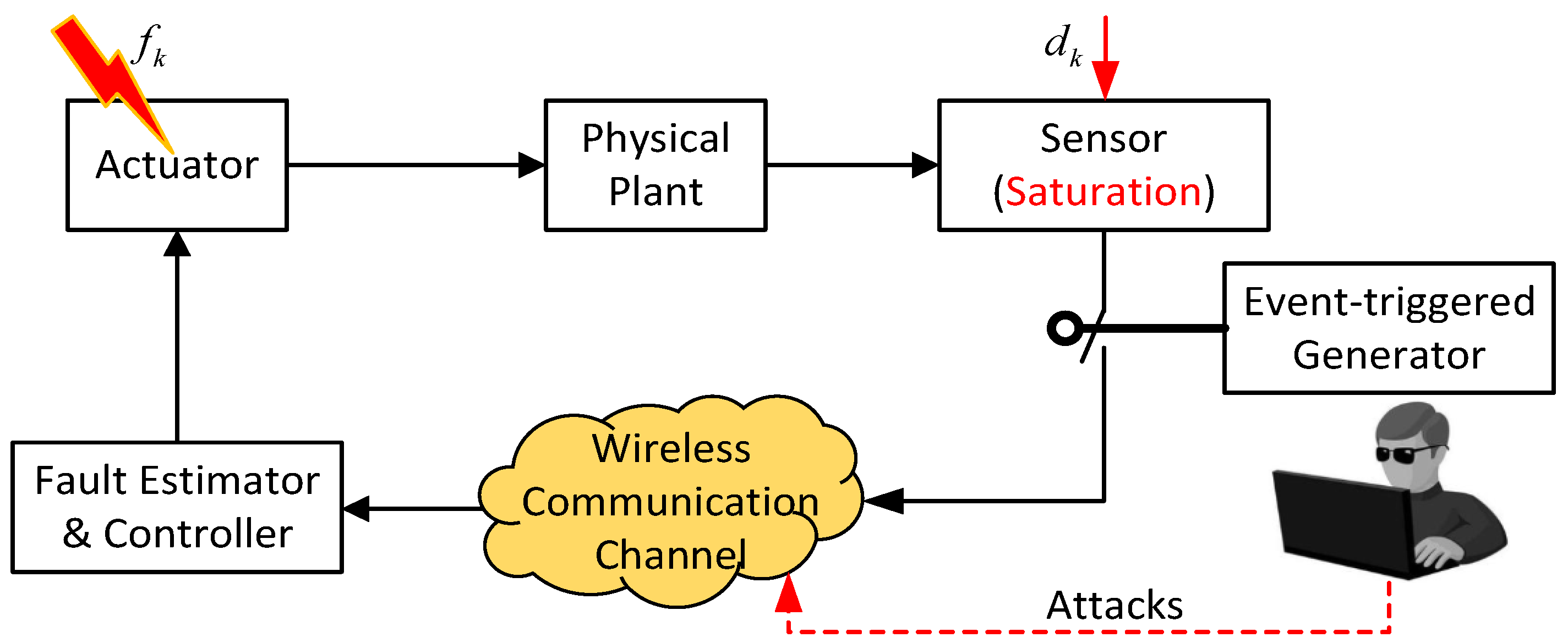
The framework of fault estimation and tolerance considered in this paper is shown in Figure 1. The CPS is described by discrete-time stochastic dynamics
x k + 1 = A 1 x k + A 2 x k w k + B u k + F f k + D 1 d k , y ¯ k = C x k + D 2 d k ,
with the time index k, system state x k R n , control input u k R q , ideal measurement y ¯ k R p , the unknown but bounded disturbances d k R n , and actuator fault f k R n , which belong to 2 0 , . A zero-mean Gaussian noise sequence w k R satisfies E w k 2 = 1 . The signals sent by the adversaries for the FDIAs are generated as
y a , k = y ¯ k + τ k ,
where τ k are also the unknown but bounded signals satisfying τ k 2 0 , . It is observed that the term τ k in (2) has a similar form to the actuator fault f k and the external disturbance d k . Consequently, it is difficult to distinguish them by using various detectors, which makes the estimator design problem more challenging.
In practical engineering, successful FDIAs occur randomly in implementation because of the physical constraints that the attackers have to face, as highlighted in Ref. [24]. Such constraints include limited-energy devices, limited-bandwidth transmission channels, and randomly fluctuating channel conditions. It is essential to take these constraints into account when developing a realistic deception attack model. Based on the discussions in the Introduction, we can rewrite the actual measurement sent by remote fault estimator as
y k = ( 1 α k ) y ¯ k + α k y a , k ,
where the stochastic scalar variable α k is a Bernoulli distributed sequence with
Prob α k = 1 = E ( α k ) = α 1 , Prob α k = 0 = E ( 1 α k ) = α 2 .
The problem of full-state saturations is a special case of system nonlinearities in physical systems. The partial state saturation phenomenon is more general than the full-state saturation in engineering practices. We mainly focus on discrete stochastic systems with partial state saturations in the present study. Now, we decompose the system (1) as
x k + 1 c = A 11 1 x k c + A 12 1 x k s + A 11 2 x k c w k + A 12 2 x k s w k + F 1 f k + D 1 1 d k + B 1 u k , x k + 1 s = σ ( A 21 1 x k c + A 22 1 x k s + A 21 2 x k c w k + A 22 2 x k s w k + F 2 f k + D 2 1 d k + B 2 u k ) , y k = ( 1 α k ) ( C 1 x k c + C 2 x k s + D 2 d k ) + α k y a , k ,
where the states of saturation-free and saturation are x k c N n s and x k s N s , respectively. The saturation function σ ( · ) R s R s is denoted as
σ ( s ˜ k ) = ( s ˜ k 1 ) T ( s ˜ k 2 ) T ( s ˜ k s ) T T ,
with σ ( s ˜ k q ) = s i g n ( s ˜ k q ) min ( s ˜ max q , s ˜ k q ) , where s ˜ k q and s ˜ max q are the q t h element of the vector s ˜ k and the saturation level, respectively. Here, sign(·) is the signum function. By revising Definition 1 in [31], we can obtain the following definition:
Definition 1. 
A nonlinear function f ( · ) : R l R l : belongs to a sector area S 1 , S 2 if
( f ( s ˜ k ) X 1 s ˜ k ) T ( f ( s ˜ k ) X 2 s ˜ k ) 0 , s ˜ k R l
for some real diagonal matrices X 1 , X 2 R l , where a positive-definite matrix X = X 2 X 1 .
Using Definition 1 and the standard loop transformation technique, supposing that there exist diagonal matrices S 1 and S 2 such that 0 < S 1 < I < S 2 ; and then, the saturated nonlinear function σ ( · ) in system (5) can be separated into linear and nonlinear components:
σ ( s k ) = S 1 s k + ψ x ( s k ) , s k = A 21 1 x k c + A 22 1 x k s + A 21 2 x k c w k + A 22 2 x k s w k + F 2 f k + D 2 1 d k + B 2 u k ,
where the nonlinear part satisfies
ψ x T ( s k ) ( ψ x ( s k ) S s k ) 0
and a positive-definite matrix S = S 2 S 1 .
As system (5) encompasses stochastic variables α k and w k , it constitutes a stochastic parameter system. Consequently, it is necessary to present the notion of mean-squared stochastic stability.
Definition 2. 
A discrete stochastic process ξ k is considered exponentially mean-squared stable if constants ζ 1 > 0 and 0 < ζ 2 < 1 exist, satisfying the following conditions:
E ξ k 2 ζ 1 ζ 2 k E ξ 0 2 , k I + .

3. An Event-Triggered Fault Estimator

In this section, an event-triggered fault estimator will be established so that the states and faults of the considered systems (5) can be reconstructed. Subsequently, the mean-squared stability analysis of the designed estimator will be explicitly provided. To this end, we temporarily ignore the control input u k in the system Equation (5) for the convenience of discussion. An event-triggered fault estimator has the following form:
x ^ k + 1 c = A 11 1 x ^ k c + A 12 1 x ^ k s + F 1 f ^ k + L 1 ( y l , k α 2 C 1 x ^ k c α 2 C 2 x ^ k s ) , x ^ k + 1 s = S 1 A 21 1 x ^ k c + S 1 A 22 1 x ^ k s + S 1 F 2 f ^ k + L 2 ( y l , k α 2 C 1 x ^ k c α 2 C 2 x ^ k s ) , f ^ k + 1 = f ^ k + L 3 ( y l , k α 2 C 1 x ^ k c α 2 C 2 x ^ k s ) ,
where the notation of “ ^ ” indicates the estimate, L i ( i = 1 , 2 a n d 3 ) are the estimation gains with appropriate dimensions to be designed, and y l , k denotes the last released measurement information that is transmitted from sensor to remote estimator. In order to conserve computational and communicative resources, an event-triggered transmission approach is utilized to determine if the measurement should be transmitted. Thus, measurement information is only required to be sent at transmission times k l with l N . The measurement information of event-triggered fault estimator can further be described as y l , k = y k l , where k k l , k l + 1 and k N .
The state estimation error dynamics of the saturated-free subsystem can be obtained by subtracting (5) from (11)
e k + 1 c = x k + 1 c x ^ k + 1 c = ( A 11 1 α 2 L 1 C 1 ) e k c + ( A 12 1 α 2 L 1 C 2 ) e k s + F 1 e k f + ( A 11 2 x k c w k + A 12 2 x k s w k ) + ( D 1 1 α 2 L 1 D 2 ) d k L 1 Δ k α 1 L 1 τ k + ( α k α ) L 1 C 1 x k c + ( α k α ) L 1 C 2 x k s + ( α k α ) L 1 D 2 d k ( α k α ) L 1 τ k ,
where e k c = x k c x ^ k c , e k s = x k s x ^ k s and e k f = f k f ^ k .
Through mathematical manipulations, the state estimation error dynamics of the saturated subsystem can be calculated as follows
e k + 1 s = x k + 1 s x ^ k + 1 s = ( S 1 A 21 1 α 2 L 2 C 1 ) e k c + ( S 1 A 22 1 α 2 L 2 C 2 ) e k s + S 1 F 2 e k f + ( S 1 A 21 2 x k c w k + S 1 A 22 2 x k s w k ) + ( S 1 D 2 1 α 2 L 2 D 2 ) d k L 2 Δ k + ψ x ( s k ) α 1 L 2 τ k + ( α k α ) L 2 C 1 x k c + ( α k α ) L 2 C 2 x k s + ( α k α ) L 2 D 2 d k ( α k α ) L 2 τ k .
Further, it is easy to show that
e k + 1 f = f k + 1 f ^ k + 1 = Δ f , k + e k f α 2 L 3 C 1 e k c α 2 L 3 C 2 e k s α 2 L 3 D 2 d k L 3 Δ k α 1 L 3 τ k + ( α k α ) L 3 C 1 x k c + ( α k α ) L 3 C 2 x k s + ( α k α ) L 3 D 2 d k ( α k α ) L 3 τ k ,
where the fault difference is defined as Δ f , k = f k + 1 f k .
Considering the above discussions, our objective is to design the fault estimator (11) with the corresponding event condition for the system (5) so that the error dynamics system is exponentially mean-squared stable, and the energy norm performance constraint is satisfied. In other words, we aim to design an estimator such that:
(1) The estimation error dynamics associated with the saturation-free state, saturated state, and fault exhibit exponential mean-squared stability;
(2) Given the zero-initial constraint, the output estimation error e y , k adheres to the subsequent criteria:
E e y , k T e y , k γ 1 2 E d ˜ k T d ˜ k < 0
for all nonzero d ˜ k and a prescribed attenuation level γ 1 > 0 , where e y , k = y l , k α 2 C 1 x ^ k c α 2 C 2 x ^ k s and d ˜ k = f k T d k T Δ f , k T τ k T T .
Remark 1. 
The design problem (1) ensures exponential stability of e k c , e k s , and e k f in the mean-squared sense. The performance function (15) ensures that the gain between d ˜ k and e y , k remains below γ 1 2 . Furthermore, d ˜ k in Equation (15) encompasses exogenous disturbances, fault signals, and false information transmitted by adversaries. Minimizing their influences is essential for the effectiveness of the fault estimator.
Theorem 1. 
Consider the partial state-saturated system (5) subject to random FDIAs. Given α 3 E α k α 2 = α 1 α , for a specified positive scalar γ 1 , if positive definite symmetric matrices P j ( j = 1 , 2 , , 5 ) , a positive scalar β and matrices R j ( j = 1 , 2 , 3 ) exist, which fulfill the subsequent constraint:
Θ = Θ ˜ 11 0 0 Θ ˜ 22 Θ ˜ 23 Θ ˜ 33 Θ ˜ 2 Θ ˜ 3 Θ ˜ 2 T < 0 ,
where
Θ ˜ 11 = P 1 0 0 0 P 2 0 0 P 3 0 1 β I ,
Θ ˜ 22 = Λ 3 Λ 5 0.5 ( S A 21 1 ) T 0 Λ 4 0.5 ( S A 22 1 ) T 0 I 0.5 S F 2 γ 1 2 I ,
Λ 3 = P 3 + C 1 T C 1 + ( A 11 2 ) T P 3 A 11 2 + ( A 21 2 ) T P 4 A 21 2 + Λ ˜ 1 , Λ ˜ 1 = ( A 11 2 ) T P 1 A 11 2 + ( S 1 A 21 2 ) T P 2 S 1 A 21 2 , Λ 4 = P 4 + C 2 T C 2 + ( A 12 2 ) T P 3 A 12 2 + ( A 22 2 ) T P 4 A 22 2 + Λ ˜ 2 , Λ ˜ 2 = ( A 12 2 ) T P 1 A 12 2 + ( S 1 A 22 2 ) T P 2 S 1 A 22 2 , Λ 5 = C 1 T C 2 + ( A 11 2 ) T P 1 A 12 2 + ( S 1 A 21 2 ) T P 2 S 1 A 22 2 , + ( A 11 2 ) T P 3 A 12 2 + ( A 21 2 ) T P 4 A 22 2 ,
Θ ˜ 23 = C 1 T D 2 0 0 C 2 T D 2 0 0 0.5 S D 2 1 0 0 0 0 0 ,
Θ ˜ 33 = Λ 6 0 0 γ 1 2 I 0 γ 1 2 I , Λ 6 = γ 1 2 I + D 2 T D 2 ,
Θ ˜ 2 = Θ ¯ 11 Θ ¯ 12 Θ ¯ 13 Θ ¯ 14 Θ ¯ 21 Θ ¯ 22 Θ ¯ 23 Θ ¯ 24 ,
Θ ¯ 11 = ( P 1 A 11 1 α 2 R 1 C 1 ) T 0 ( P 1 A 12 1 α 2 R 1 C 2 ) T 0 F 1 T P 1 T 0 R 1 T 0 0 ( R 1 C 1 ) T 0 ( R 1 C 2 ) T ,
Θ ¯ 21 = 0 0 0 0 ( P 1 D 1 1 α 2 R 1 D 2 ) T ( R 1 D 2 ) T 0 0 α 1 R 1 T R 1 T ,
Θ ¯ 12 = ( P 2 S 1 A 21 1 α 2 R 2 C 1 ) T 0 ( P 2 S 1 A 22 1 α 2 R 2 C 2 ) T 0 ( S 1 F 2 ) T P 2 T 0 R 2 T 0 0 ( R 2 C 1 ) T 0 ( R 2 C 2 ) T ,
Θ ¯ 22 = P 2 T 0 0 0 ( P 2 S 1 D 2 1 α 2 R 2 D 2 ) T ( R 2 D 2 ) T 0 0 α 1 R 2 T R 2 T ,
Θ ¯ 13 = α 2 C 1 T R 3 T 0 0 α 2 C 2 T R 3 T 0 0 P 3 T 0 0 R 3 T 0 0 0 C 1 T R 3 T ( A 11 1 ) T P 4 T 0 C 2 T R 3 T ( A 12 1 ) T P 4 T ,
Θ ¯ 23 = 0 0 0 0 0 F 1 T P 4 T α 2 D 2 T R 3 T D 2 T R 3 T ( D 1 1 ) T P 4 T P 3 T 0 0 α 1 R 3 T R 3 T 0 ,
Θ ¯ 14 = 0 α 2 C 1 T 0 0 α 2 C 2 T 0 0 0 0 0 I 0 ( S 1 A 21 1 ) T P 5 T 0 C 1 T ( S 1 A 22 1 ) T P 5 T 0 C 2 T ,
Θ ¯ 24 = P 5 T 0 0 ( S 1 F 2 ) T P 5 T 0 0 ( S 1 D 2 1 ) T P 5 T ( α 2 D 2 ) T D 2 T 0 0 0 0 α 1 I I ,
Θ ˜ 3 = d i a g P 1 1 , α 3 P 1 1 , P 2 1 , α 3 P 2 1 , P 3 1 , α 3 P 3 1 , P 4 1 , P 5 1 , I , α 3 I .
Then, the proposed event-triggered fault estimator (11) can be implemented such that the state and fault estimation errors are exponentially mean-squared stable, using the following event condition:
Δ k T Δ k y ¯ k T y ¯ k < β .
Estimator gains can be determined by L 1 = P 1 1 R 1 , L 2 = P 2 1 R 2 , and L 3 = P 3 1 R 3 . Moreover, the output estimation error e y , k satisfies
E e y , k T e y , k γ 1 2 E d ˜ k T d ˜ k < 0
for all nonzero d ˜ k , where e y , k = y l , k α 2 C 1 x ^ k c α 2 C 2 x ^ k s and d ˜ k = f k T d k T Δ f , k T τ k T T .
Proof. 
Consider the following Lyapunov function: V k = i = 1 5 Δ V k i where V k 1 = ( e k c ) T P 1 e k c , V k 2 = ( e k s ) T P 2 e k s , V k 3 = ( e k f ) T P 3 e k f , V k 4 = ( x k c ) T P 4 x k c , and V k 5 = ( x k s ) T P 5 x k s . Using the estimation error dynamics (12)–(14), it can be formulated that
Δ V k 1 = E ( e k + 1 c ) T P 1 e k + 1 c ( e k c ) T P 1 e k c , Δ V k 2 = E ( e k + 1 s ) T P 2 e k + 1 s ( e k s ) T P 2 e k s , Δ V k 3 = E ( e k + 1 f ) T P 3 e k + 1 f ( e k f ) T P 3 e k f , Δ V k 4 = E ( x k + 1 c ) T P 4 x k + 1 c ( x k c ) T P 4 x k c , Δ V k 5 = E ( x k + 1 s ) T P 5 x k + 1 s ( x k s ) T P 4 x k s .
Taking Equations (8), (9), and (32) into consideration, we have
Δ V k i = 1 5 Δ V k i ψ x T ( s k ) ψ x ( s k ) + ψ x T ( s k ) S A 21 1 x k c + ψ x T ( s k ) S A 22 1 x k s + ψ x T ( s k ) S F 2 f k + ψ x T ( s k ) S D 2 1 d k 1 β Δ k T Δ k + ( x k c ) T C 1 T C 1 x k c + ( x k s ) T C 2 T C 2 x k s + d k T D 2 T D 2 d k + 2 ( x k c ) T C 1 T C 2 x k s + 2 ( x k c ) T C 1 T D 2 d k + 2 ( x k s ) T C 2 T D 2 d k = ς k T Θ ς k ,
where ς k = ς ˜ k T d ˜ k T T , d ˜ k = f k T d k T Δ f , k T τ k T T and ς ˜ k = e k c T e k s T e k f T Δ k T x k c T x k s T ψ x T s k T . Based on condition (16), without considering the influence of d ˜ k , the following inequality can be deduced:
Δ V k ς ˜ k T Θ ς ˜ k λ min Θ ς ˜ k T ς ˜ k < θ 1 ς ˜ k T ς ˜ k ,
where 0 < θ 1 < min λ min Θ , θ 2 , θ 2 = max λ max ( P j ) and j = 1 , 2 , , 5 . From (36), we can further obtain
Δ V k < θ 1 ς ˜ k T ς ˜ k < θ 1 e ˜ k T e ˜ k < θ 1 θ 2 V k ,
where e ˜ k = ( e k c ) T ( e k s ) T ( e k f ) T T . Therefore, according to Definition 1, it can be verified from the results in Refs. [6,8] that the exponentially mean-squared stability of both state estimation error and fault estimation error is ensured. Next, consider system (5) with d ˜ k 0 . We introduce the following energy-norm index:
J 1 = Δ V k + E e y , k T e y , k γ 1 2 E d ˜ k T d ˜ k = Δ V k + α 2 2 ( e k c ) T C 1 T C 1 e k c + α 2 2 ( e k s ) T C 2 T C 2 e k s + α 2 2 d k T D 2 T L 3 T L 3 D 2 d k + Δ k T Δ k + α 1 2 τ k T τ k + α 3 ( x k c ) T C 1 T C 1 x k c + α 3 ( x k s ) T C 2 T C 2 x k s + α 3 d k T D 2 T D 2 d k + α 3 τ k T τ k + 2 α 2 2 ( e k c ) T C 1 T C 2 e k s + 2 α 2 2 ( e k c ) T C 1 T L 3 D 2 d k + 2 α 2 ( e k c ) T C 1 T Δ k + 2 α 1 α 2 ( e k c ) T C 1 T τ k + 2 α 2 2 ( e k s ) T C 2 T L 3 D 2 d k + 2 α 2 ( e k s ) T C 2 T Δ k + 2 α 1 α 2 ( e k s ) T C 2 T τ k + 2 α 2 d k T D 2 T L 3 T Δ k + 2 α 1 α 2 d k T D 2 T L 3 T τ k + 2 α 1 Δ k T τ k + 2 α 3 ( x k c ) T C 1 T C 2 x k s + 2 α 3 ( x k c ) T C 1 T D 2 d k 2 α 3 ( x k c ) T C 1 T τ k + 2 α 3 ( x k s ) T C 2 T D 2 d k 2 α 3 ( x k s ) T C 2 T τ k 2 α 3 d k T D 2 T τ k γ 1 2 d ˜ k T d ˜ k = ς k T Θ ς k .
Again, the use of (16) implies that Θ < 0 , and thereby J 1 < 0 . With the zero initial condition, it is straightforward to deduce Equation (15).    □
As mentioned in the Introduction, when sensors obtain measurement information, the event-triggered transmission scheme is responsible for deciding whether to send it to the remote fault estimator or not. Let γ k 0 , 1 represent the sensor’s decision to transmit measurement information γ k = 1 or not γ k = 0 . From Theorem 1, it is evident that the case of sending measurement information is not included in the proof of Theorem 1. For comprehensiveness, the design presented in Theorem 1 can be readily generalized to the scenario where γ k = 1 , as articulated in the subsequent corollary.
Corollary 1. 
Consider that Δ k = 0 and Theorem 1 holds. If there are positive definite symmetric matrices P j ( j = 1 , 2 , , 5 ) , a positive scalar β, and matrices R j ( j = 1 , 2 , 3 ) that satisfy the condition (16), then the estimator (11) can ensure that the estimation errors in the state and fault are exponentially mean-squared stable when γ k = 1 . Thus, estimator gains can be determined by L 1 = P 1 1 R 1 , L 2 = P 2 1 R 2 , and L 3 = P 3 1 R 3 . Output estimation error e y , k satisfies that E e y , k T e y , k γ 1 2 E d ˜ k T d ˜ k < 0 for all nonzero d ˜ k .
Proof. 
The proof of Corollary 1 is similar to the proof of Theorem 1. Hence, the derivation of Corollary 1 is omitted in the proof.    □
Remark 2. 
It should be noted that the fault difference term Δ f , k is not neglected. Because of the occurrence of the time-varying faults in many practical systems, its effect is minimized for estimation performance by employing the H technique in the proof of Theorem 1. This implies that the designed fault estimator (11) can robustly estimate time-varying faults. By assuming that Δ f , k = 0 in (16), the desired fault estimator can also estimate constant actuator faults occurring in the considered system. Consequently, the desired fault estimator can achieve the reconstruction of both constant and time-varying actuator faults in the mean-squared sense.
Remark 3. 
The introduced event condition (32) can be referred to as the send-on-delta decision rule [32], where the difference between the current and last-transmitted information is utilized. Compared to the existing event-triggered method in Ref. [9], the proposed communication scheme does not rely on a copy of the remote estimator, which can further reduce the computational burden.

4. An Fault-Tolerant Controller Based on the Estimated Information

Generally, actuator faults can be described as additive or multiplicative external signals, which may change the model structure and increase the instability of the controlled plant. To reduce the effects of actuator fault, we introduce the estimated states x ^ k c , x ^ k s and estimated faults f ^ k to the feedback control loop, i.e.,
u k = K 1 K 2 x ^ k c x ^ k s F 1 F 2 f ^ k ,
where K 1 and K 2 are the controller gains and are designed later on. Prior to designing controller gains and analyzing the stability of the proposed controller (39), the following well-established assumption needs to be considered.
Assumption A1. 
It is supposed that B i = F i , where i = 1 and 2.
Recalling the decomposition (5) of the partial state-saturated systems, the resulting closed-loop systems with the reconfigured law (39) can be reformulated as follows
x k + 1 c = ( A 11 1 F 1 K 1 ) x k c + ( A 12 1 F 1 K 2 ) x k s + F 1 K 1 e k c + F 1 K 2 e k s + F 1 e k f + A 11 2 x k c w k + A 12 2 x k s w k + D 1 1 d k , x k + 1 s = S 1 s ¯ k + ψ x ( s ¯ k ) , s ¯ k = ( A 21 1 F 2 K 1 ) x k c + ( A 22 1 F 2 K 2 ) x k s + F 2 K 1 e k c + F 2 K 2 e k s + F 2 e k f + A 21 2 x k c w k + A 22 2 x k s w k + D 2 1 d k .
It is now ready to design the controller gains K 1 and K 2 so that the closed-loop system (40) exhibits exponential mean-squared stability.
Theorem 2. 
Consider that Theorem 1 is valid. Given a positive scalar γ 2 , the system dynamics described in (40) are considered exponentially mean-squared stable with a performance index E y k T y k < γ 2 2 E d ¯ k T d ¯ k if there exist positive definite symmetric matrices Z 1 , Z 2 and matrices R ˜ 1 , R ˜ 2 that satisfy the following condition:
Ξ 1 = Ξ ˜ 1 Ξ ˜ 2 Ξ ˜ 3 < 0 ,
where
Ξ ˜ 1 = Z 1 0 H 1 0 0 Z 2 H 2 0 0 2 I ( S D 2 1 ) T 0 γ 2 2 I 0 ( γ 2 2 + α ) I ,
H 1 = ( S A 21 1 Z 1 S F 2 R ˜ 1 ) T ,
Ξ ˜ 2 = Ξ ¯ 1 Ξ ¯ 2 ,
Ξ ¯ 1 = A 11 1 Z 1 F 1 R ˜ 1 T ( S 1 A 21 1 Z 1 S 1 F 2 R ˜ 1 ) T A 12 1 Z 2 F 1 R ˜ 2 T ( S 1 A 22 1 Z 2 S 1 F 2 R ˜ 2 ) T 0 I D 1 1 T ( S 1 D 2 1 ) T 0 0 ,
Ξ ¯ 2 = ( A 11 2 Z 1 ) T Z 1 T ( A 21 2 ) T S 1 T Z 1 T C 1 T ( A 12 2 Z 2 ) T Z 2 T ( A 22 2 ) T S 1 T Z 2 T C 2 T 0 0 0 0 0 D 2 T 0 0 0 ,
Ξ ˜ 3 = d i a g Z 1 , Z 2 , Z 1 , Z 2 , ( 1 α ) 1 I .
Furthermore, the controller gains K 1 and K 2 can be computed that K 1 = R ˜ 1 Z 1 1 and K 2 = R ˜ 2 Z 2 1 , respectively.
Proof. 
First, it is noteworthy that the partial state-saturated system (40) is exponentially mean-squared stable for d ¯ k = 0 if Equation (41) holds. A Lyapunov function is defined as
V ˜ k = ( x k c ) T Q 1 x k c + ( x k s ) T Q 2 x k s + η 0 V k ,
where V k is defined in Theorem 1, η 0 is a positive scalar, Q 1 and Q 2 are positive definite symmetric matrices. For simplicity, denote
F ˜ 1 = F 1 K 1 F 1 K 2 F 1 , F ˜ 2 = S 1 F 2 K 1 S 1 F 2 K 2 S 1 F 2 , F ˜ 3 = F 2 K 1 F 2 K 2 F 2 , G ˜ 1 = A 11 1 F 1 K 1 A 12 1 F 1 K 2 0 D 1 1 0 , G ˜ 3 = 0 0 S 0 0 , G ˜ 2 = S 1 A 21 1 S 1 F 2 K 1 S 1 A 22 1 S 1 F 2 K 2 S 1 S 1 D 2 1 0 , e ˜ k = ( e k c ) T ( e k s ) T ( e k f ) T T , x ˜ k = ( x k c ) T ( x k s ) T ψ x T ( s ¯ k ) d ¯ k T T , d ¯ k = d k T τ k T T .
Substituting Equation (40) into Equation (48) yields
Δ V ˜ k = E V ˜ k + 1 V ˜ k x ˜ k T G ˜ 1 T Q 1 G ˜ 1 x ˜ k + e ˜ k T F ˜ 1 T Q 1 F ˜ 1 e ˜ k + 2 x ˜ k T G ˜ 1 T Q 1 F ˜ 1 e ˜ k + x ˜ k T G ˜ 2 T Q 2 G ˜ 2 x ˜ k + e ˜ k T F ˜ 2 T Q 2 F ˜ 2 e ˜ k + 2 x ˜ k T G ˜ 2 T Q 2 F ˜ 2 e ˜ k + ( x k c ) T ( A 11 2 ) T Q 1 A 11 2 x k c + ( x k s ) T ( A 12 2 ) T Q 1 A 12 2 x k s + 2 ( x k s ) T ( A 12 2 ) T Q 1 A 11 2 x k c ( x k c ) T Q 1 x k c + ( x k c ) T ( A 21 2 ) T S 1 T Q 2 S 1 A 21 2 x k c + ( x k s ) T ( A 22 2 ) T S 1 T Q 2 S 1 A 22 2 x k s + 2 ( x k c ) T ( A 21 2 ) T S 1 T Q 2 S 1 A 22 2 x k s ( x k s ) T Q 2 x k s .
From Definition 1, it can be further obtained that
Δ V ˜ k = E V ˜ k + 1 V ˜ k x ˜ k T G ˜ 1 T Q 1 G ˜ 1 x ˜ k + e ˜ k T F ˜ 1 T Q 1 F ˜ 1 e ˜ k + 2 x ˜ k T G ˜ 1 T Q 1 F ˜ 1 e ˜ k + x ˜ k T G ˜ 2 T Q 2 G ˜ 2 x ˜ k + e ˜ k T F ˜ 2 T Q 2 F ˜ 2 e ˜ k + 2 x ˜ k T G ˜ 2 T Q 2 F ˜ 2 e ˜ k + ( x k c ) T ( A 11 2 ) T Q 1 A 11 2 x k c + ( x k s ) T ( A 12 2 ) T Q 1 A 12 2 x k s + 2 ( x k s ) T ( A 12 2 ) T Q 1 A 11 2 x k c ( x k c ) T Q 1 x k c + ( x k c ) T ( A 21 2 ) T S 1 T Q 2 S 1 A 21 2 x k c + ( x k s ) T ( A 22 2 ) T S 1 T Q 2 S 1 A 22 2 x k s + 2 ( x k c ) T ( A 21 2 ) T S 1 T Q 2 S 1 A 22 2 x k s ( x k s ) T Q 2 x k s ψ x T ( s ¯ k ) ψ x ( s ¯ k ) + ψ x T ( s ¯ k ) ( S A 21 1 S F 2 K 1 ) x k c + ψ x T ( s ¯ k ) ( S A 22 1 S F 2 K 2 ) x k s + ψ x T ( s ¯ k ) S F 2 K 1 e k c + ψ x T ( s ¯ k ) S F 2 K 2 e k s + ψ x T ( s ¯ k ) S F 2 e k f + ψ x T ( s ¯ k ) S D 2 1 d k η 0 θ 1 e ˜ k 2 η 1 x ˜ k 2 η 0 θ 1 η 3 e ˜ k 2 + η 2 x ˜ k e ˜ k ,
where Ξ 2 = G ˜ 1 T Q 1 F ˜ 1 + G ˜ 2 T Q 2 F ˜ 2 + G ˜ 3 T F ˜ 3 , Ξ 3 = i = 1 2 F ˜ i T Q i F ˜ i , η 1 = λ min ( Ξ 1 ) , η 2 = 2 λ min ( Ξ 2 ) , and η 3 = λ min ( Ξ 3 ) .
Selecting η 0 η 2 2 + η 1 η 3 η 1 θ 1 and from Equation (51), it can be derived that
Δ V ˜ k η 1 x ˜ k 2 η 0 θ 1 η 3 e ˜ k 2 + η 1 η 0 θ 1 η 3 x ˜ k e ˜ k η 1 2 x ˜ k 2 1 2 η 0 θ 1 η 3 e ˜ k 2 < 0 .
As with the proof of Theorem 1, the proposed controller can guarantee that the closed-loop system (40) is exponential mean-squared stable when d ¯ k = 0 . In the next step, the following performance index (53) is designed to relieve the influence of d ¯ k :
J 2 = E k = 0 β 1 y k T y k γ 2 2 E k = 0 β 1 d ¯ k T d ¯ k ,
where β is an arbitrary positive integer. According to the zero initial condition and Equation (51), we have
E y k T y k γ 2 2 E d ¯ k T d ¯ k + Δ V ˜ k = Δ V ˜ k + ( 1 α ) x k c T C 1 T C 1 x k c + x k s T C 2 T C 2 x k s + ( 1 α ) d k T D 2 T D 2 d k + 2 ( 1 α ) x k c T C 1 T C 2 x k s + 2 ( 1 α ) x k c T C 1 T D 2 d k + 2 ( 1 α ) x k s T C 2 T D 2 d k + α τ k T τ k γ 2 2 d ¯ k T d ¯ k η 0 θ 1 e ˜ k 2 η 1 2 x ˜ k 2 1 2 η 0 θ 1 η 3 e ˜ k 2
for all nonzero d ¯ k 2 0 , . Notice that the performance constraint J 2 is met if Ξ 1 < 0 .    □
Remark 4. 
Note that at this stage, the inequality Ξ 1 in Equation (54) is not in a standard computational form. Hence, it is challenging to solve Equation (54) directly using a MATLAB computation toolbox. By applying the Schur complement and pre- and post-multiplying Ξ 1 in Equation (54) by d i a g Q 1 1 , Q 2 1 , I , it can be easily verified that the inequality Ξ 1 in Equation (54) is equivalent to the Equation (41), where Z 1 = Q 1 1 and Z 2 = Q 2 1 . Furthermore, J 1 and J 2 are utilized to attenuate the unwanted factors containing exogenous disturbances, fault signals, and false information sent by attackers. This kind of performance function is typically made in the field of fault diagnosis theory with the H technique.
Remark 5. 
The motivation on this research is based on our prior work in Ref. [33], where we studied the issue of event-triggered fault estimation for state-delayed stochastic CPSs. There are three main differences between these two studies: first, this paper focuses on partial state-saturated CPSs subjected to additive actuator faults, while Ref. [33] investigated state-delayed stochastic CPSs with sensor failures and random sensor nonlinearities; second, this paper introduces a set of reduced-order fault estimators independent from the corresponding fault-tolerant controller design, utilizing the separation principle and decomposition technique. In contrast, Ref.  [33] designed an event-triggered fault estimator to address sensor faults through an augmentation approach; finally, the present study explores the random influence of FDIAs on measurement outputs by employing a stochastic variable that conforms to the Bernoulli distribution, whereas the problem of randomly occurring FDIAs was not considered in Ref. [33].

5. Experimental Studies

The effectiveness of the proposed approach is demonstrated on a platform that represents a networked CPS over a shared wireless channel. The estimation task aims to estimate both state and fault under the proposed event-triggered transmission scheme, while the control task focuses on compensating for the fault effect on the partial state-saturated system. The performance of the proposed method is compared with that of the classical fault estimator and fault-tolerant controller.

5.1. Experimental Setup

Based on the theoretical results we derived, a complete algorithm of the event-triggered remote fault estimation and accommodation are summarized in Algorithm 1.
Note that wireless transceiver modules typically consume more energy than computation modules in most industrial applications. Hence, it is worthwhile to develop an energy-efficient transmission scheme for wireless nodes. As can be seen from Algorithm 1, the designed estimation strategy at each time instant is divided into two parts. If the condition γ k = 0 is satisfied, then the state estimation and fault estimation steps can use y l , k instead of the current measurement data. Such an operation allows the wireless transceiver modules to not send information to the remote receiver at the current time instant so as to prolong the battery life of the wireless sensor nodes. In contrast, if the condition γ k = 1 is satisfied, the state estimation and fault estimation steps will use the current measurement information y k to ensure the reconstruction accuracy of state and fault.
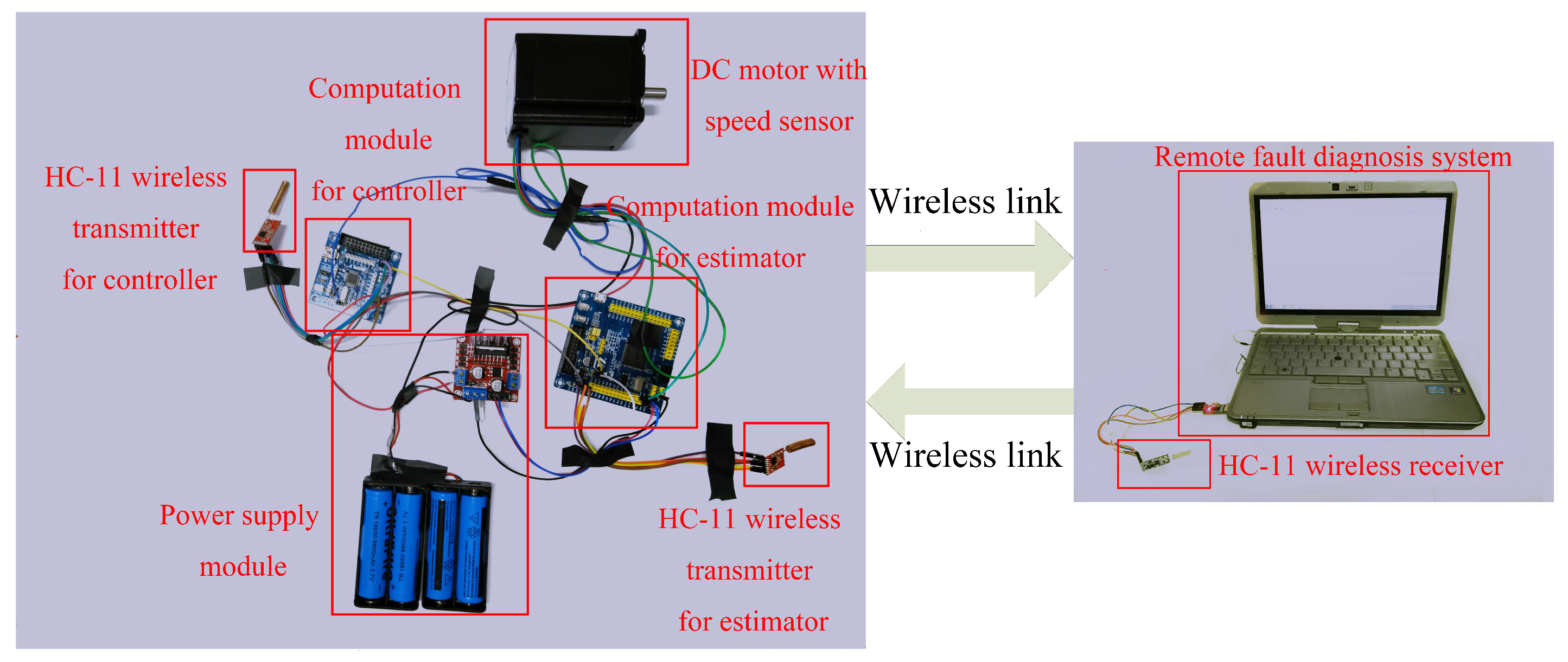
In order to verify the effectiveness of Algorithm 1, this study employs the experimental platform of the DC motor constructed in Figure 2. A speed sensor and a type of wireless nodes are positioned to construct a wireless network for transmitting motor speed information from the sensor side to a remote fault diagnosis system. The estimated information is then transmitted to a local wireless node, enabling the remote fault diagnosis system to accommodate fault effects. The wireless node comprises the following components: (1) the wireless transceiver module HC-11 can realize the mutual conversion between serial port data and radio frequency signals, which also has the characteristics of low power consumption, small size, and radio frequency stability. (2) The computation module STM32L162ZD is a high-performance microcontroller unit. (3) The power supply module converts AC power to DC power and provides stable working power for wireless modules. The wireless transceiver module HC-11 is responsible for transmitting the motor speed signal collected by the speed sensor to the remote fault diagnosis system. The computation module STM32L162ZD determines when to transmit the data packet according to the proposed event-triggered decision rule. Once the event condition is triggered, the computation module sends the measurement information to the HC-11 wireless transceiver module. The power supply module provides a stable working voltage for the wireless transceiver module and the computation module to ensure their normal operation. Through the mutual cooperation of the above modules, the fault diagnosis system can calculate the fault and state values according to the designed estimator, and send the feedback control signals to the wireless node for the DC motor to achieve fault tolerance.
Algorithm 1: Recursive algorithm of the event-triggered remote fault estimation and fault-tolerant control.
Set the initial conditions x ^ 0 c , x ^ 0 s , f ^ 0 , γ 0 = 1 and k = 0 ;
1:
At each time instant k, the following steps are executed:
2:
if Δ k T Δ k y ¯ k T y ¯ k < β then
3:
     γ k = 0 , the current measurement information cannot be sent out to achieve energy-saving;
4:
    State estimation step:
5:
     y ^ k = α 2 C 1 x ^ k c + α 2 C 2 x ^ k s ;
6:
     x ^ k + 1 c = A 11 1 x ^ k c + A 12 1 x ^ k s + F 1 f ^ k + L 1 ( y l , k y ^ k ) ;
7:
     x ^ k + 1 s = S 1 A 21 1 x ^ k c + S 1 A 22 1 x ^ k s + S 1 F 2 f ^ k + L 2 ( y l , k y ^ k ) ;
8:
    Fault estimation step:
9:
     f ^ k + 1 = f ^ k + L 3 ( y l , k y ^ k ) ;
10:
else
11:
     γ k = 1 , the remote estimator can obtain current measurement information to ensure robust estimation;
12:
    State estimation step:
13:
     y ^ k = α 2 C 1 x ^ k c + α 2 C 2 x ^ k s ;
14:
     x ^ k + 1 c = A 11 1 x ^ k c + A 12 1 x ^ k s + F 1 f ^ k + L 1 ( y k y ^ k ) ;
15:
     x ^ k + 1 s = S 1 A 21 1 x ^ k c + S 1 A 22 1 x ^ k s + S 1 F 2 f ^ k + L 2 ( y k y ^ k ) ;
16:
    Fault estimation step:
17:
     f ^ k + 1 = f ^ k + L 3 ( y k y ^ k ) ;
18:
end if
19:
Fault-tolerant control step:
20:
u k = K 1 K 2 x ^ k c x ^ k s F 1 F 2 f ^ k ;

5.2. DC Motor: Description and Modeling

The DC motor’s dynamics model is modeled in Ref. [33] as
i ˙ a ω ˙ = R a L a C e L a C m J e f m J e i a ω + 1 L a 0 u a , ω = 0 1 i a ω ,
where coefficient ω is the rotor speed, J e is the rotor inertia, C e is the back electromotive force constant, f m is the viscous friction coefficient, C m is the torque constant, and u a is the motor armature voltage input. The current, inductance, and resistance of the motor armature are separately expressed as i a , L a and R a . Furthermore, i ˙ a and ω ˙ represent the first-order derivative of i a and ω , respectively. In this experiment, we employ a 100 W DC motor that has a rated current of 3 A and a rated voltage of 24 V. Taking into account the main technical specifications of the DC motor, the discretized model of system (55) with a sampling time of 0.01 s is formulated as follows
i a , k + 1 ω k + 1 0 . 96 0.03 0.129 0 . 9173 i a , k ω k + 0.0115 0.021 u k , y k = 0 1 i a , k ω k .
The second state of rotor speed is subject to a saturation constraint, and the saturation function σ ( s k ) is obtained as follows
σ s k = s k , i f s max s k s max ; σ s k = s max , i f s k > s max ; σ s k = s max , i f s k < s max .
In this setup, the saturation value s max is set as 0.02, S 1 = 0.8 and S = 0.2 . The probability of FDIAs is assumed as 2 % . The exogenous disturbance d k is selected as 0.05 s i n 0.1 k , and the attack signal τ k is set as 0.7 e k . Other matrices in system (1) are parameterized as follows
A 2 = 0.13 0.01 0 0.17 , D 1 = 0.2 0.15 , D 2 = 0.12 .
Now, the original system (1) can be transformed into the following two subsystems:
x k + 1 c = 0.96 x k c 0.03 x k s + 0.13 x k c w k + 0.01 x k s w k + 0.0115 f k + u k + 0.2 d k , y k = ( 1 α k ) ( x k s + 0.12 d k ) + α k τ k ,
and
x k + 1 s = σ ( 0.129 x k c + 0.9173 x k s + 0.17 x k s w k + 0.021 f k + u k + 0.15 d k ) , y k = ( 1 α k ) ( x k s + 0.12 d k ) + α k τ k .
Choosing γ 1 = 0.95 , γ 2 = and β = 10 2 , the event-triggered fault estimator and fault-tolerant controller are constructed as follows
x ^ k + 1 c = 0.96 x ^ k c 0.03 x ^ k s + 0.0115 f ^ k + 0.0327 ( y l , k 0.98 x ^ k s ) , x ^ k + 1 s = 0.1032 x ^ k c + 0.73384 x ^ k s + 0.129 ( y l , k 0.98 x ^ k s ) , f ^ k + 1 = f ^ k + 0.864 ( y l , k 0.98 x ^ k s ) , u k = 0.0497 0.0197 x ^ k c x ^ k s 0.0115 0 f ^ k .

5.3. Experimental Results

To demonstrate the effectiveness of the proposed methods, a series of experiments are presented in this subsection.
Experiment 1: Effectiveness and Robustness of the State Estimation
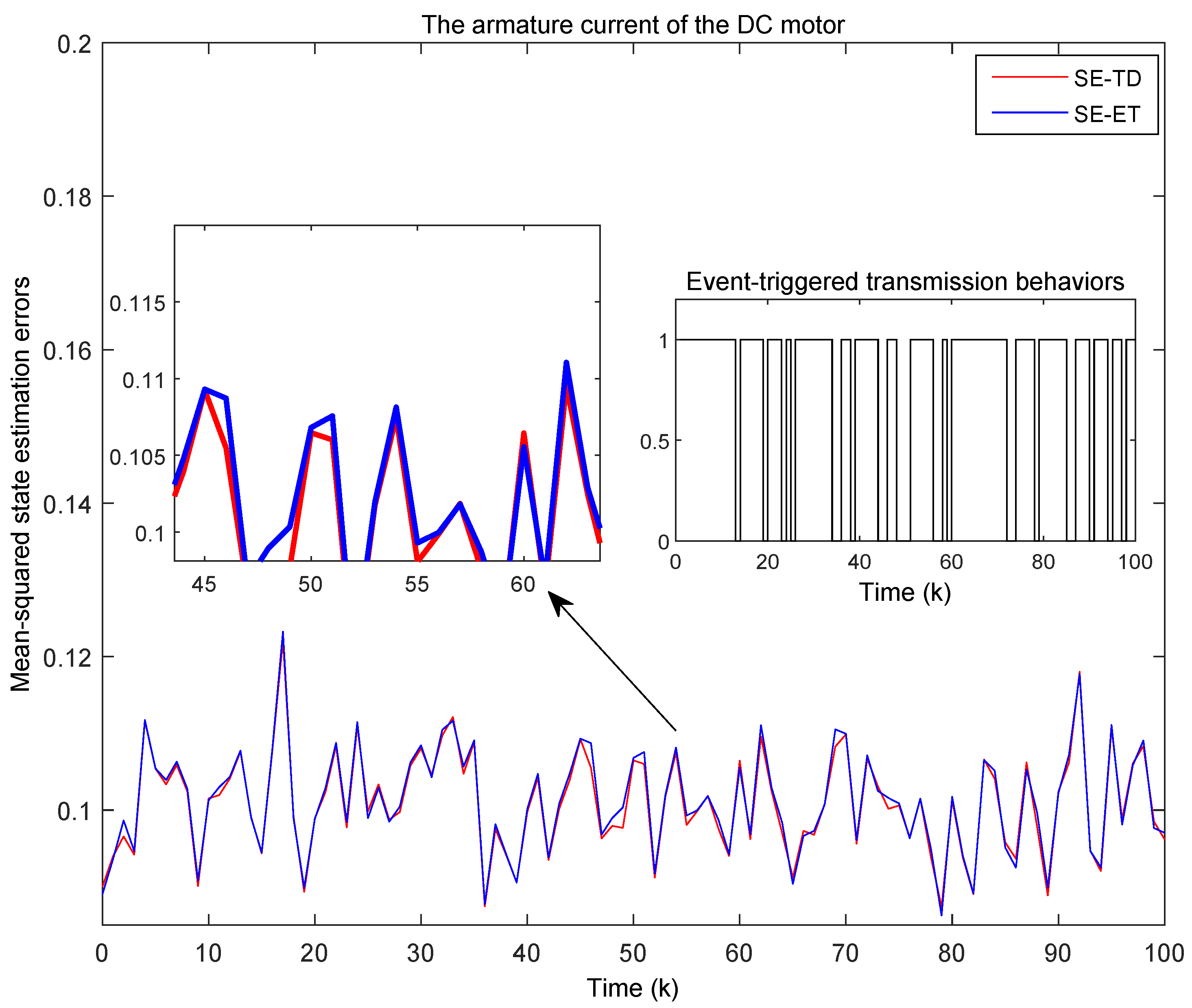
The first experiment aims to assess the effectiveness of state estimation by implementing the proposed event-triggered data transmission scheme. The mean-squared state estimation error trajectories are shown in Figure 3 and Figure 4 to compare the designed event-triggered state estimator (SE-ET) and the estimator using time-driven data transmission scheme (SE-TD). The corresponding transmission behaviors are also illustrated in the above figures. As shown in Figure 3 and Figure 4, the state estimation trajectories of the two approaches, namely SE-ET and SE-TD, almost overlap with the increase of time. Evidently, the state estimation accuracy is not affected by the event-triggered data transmission scheme. However, it should be noted that in the particular case where the triggering condition parameter γ k takes the value of zero, the mean-squared state estimation error achieved by SE-ET is marginally greater than that calculated by SE-TD, which is also consistent with the result of Theorem 1.
In order to verify the security of the designed event-triggered estimator, the mean-squared state estimation errors are examined subject to the different attack probabilities. Figure 5 displays the curves on the mean-squared state estimation error of system state 1 corresponding to increased α 1 . It can be observed from Figure 5 that the mean-squared state estimation error shows a steady upward trend with the increase of α 1 . Meanwhile, it is apparent that a higher frequency of attacks leads to a slight deterioration in the state estimation performance. The first experiment demonstrates that the proposed state estimator can achieve a satisfactory estimation performance using an event-triggered data transmission scheme.
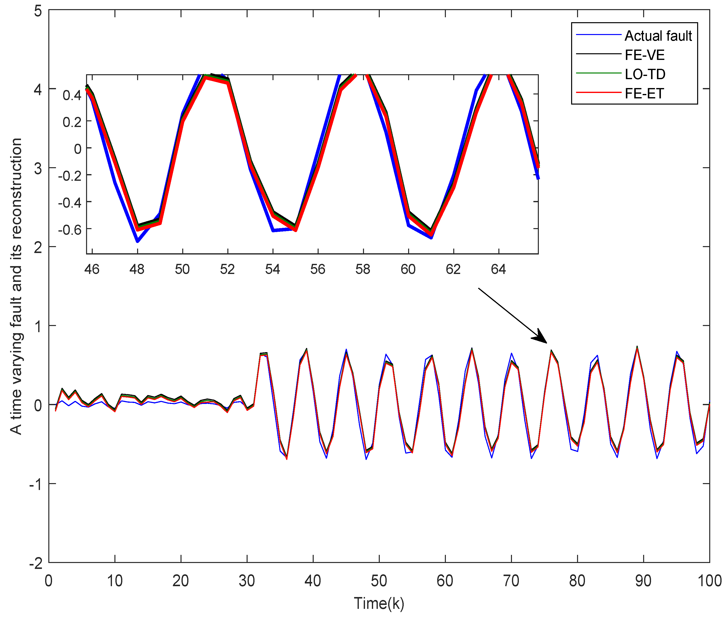
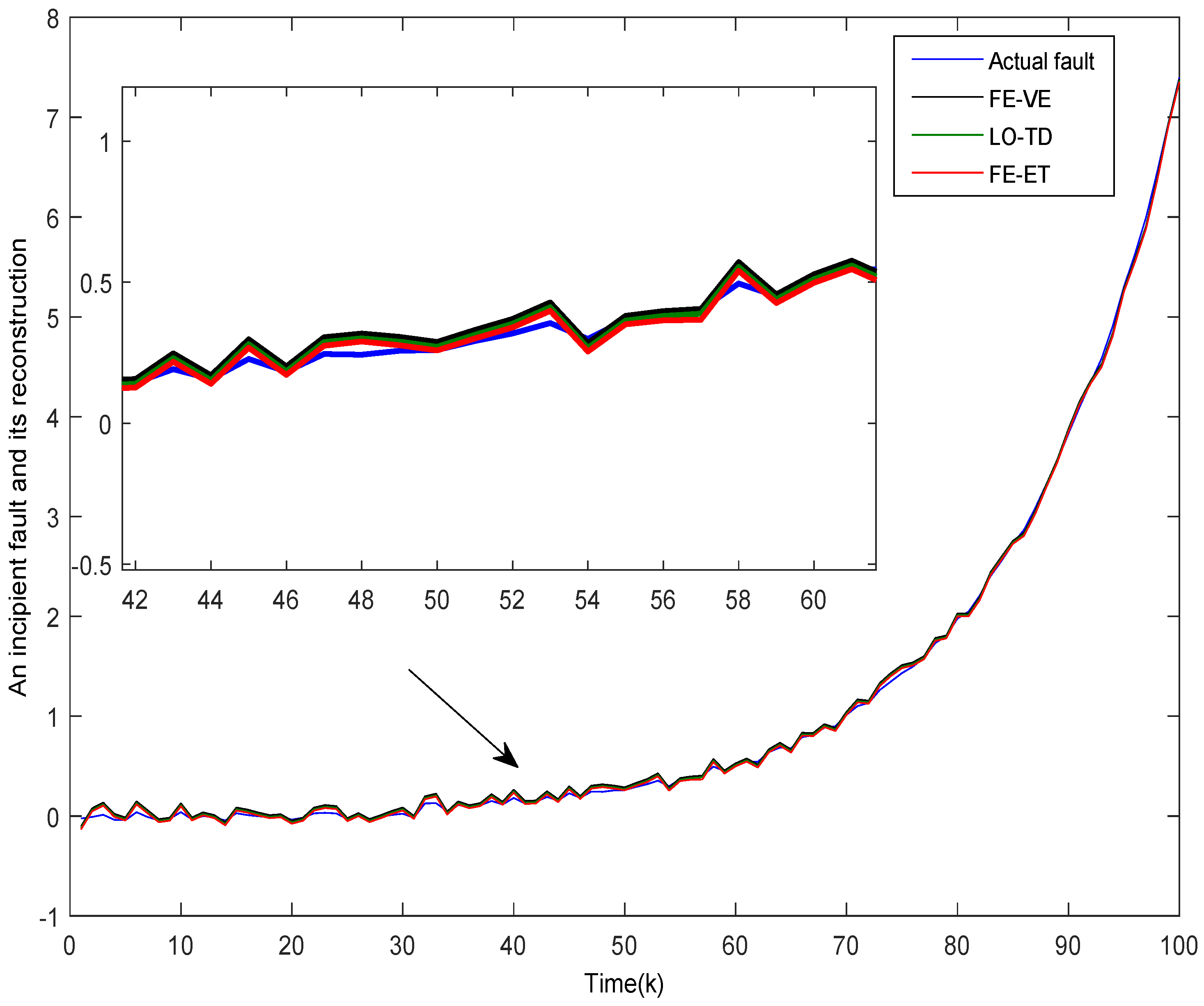
Experiment 2: Effectiveness and Robustness of Fault Estimation
Here, three fault scenarios are considered as follows:
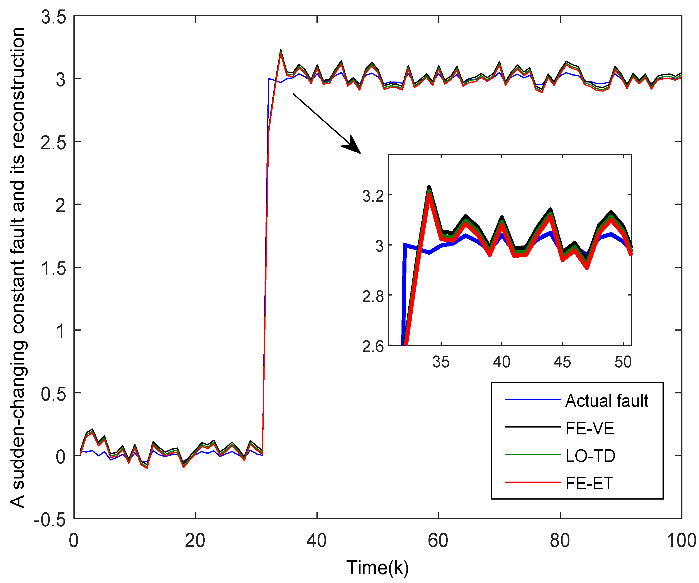
A suddenly changing constant fault
f k = 0 k 30 , 3 k > 30 ,
A time-varying fault
f k = 0 k 30 , 0.7 cos k k > 30 ,
Finally, an incipient fault
f k = 0 k 30 , 0.01 e 0.0667 k k > 30 .
By using the proposed event-triggered fault estimator (FE-ET) in (61), Figure 6, Figure 7 and Figure 8 illustrate the actual and reconstructed signals of the suddenly changing constant fault, the time-varying fault, and the incipient fault, respectively. For comparison, the reconstructed fault signals using the time-driven learning observer (LO-TD) and the variance-constrained event-triggered fault estimator (VE-FE) borrowed from Refs. [28,34] are also depicted in Figure 6, Figure 7 and 
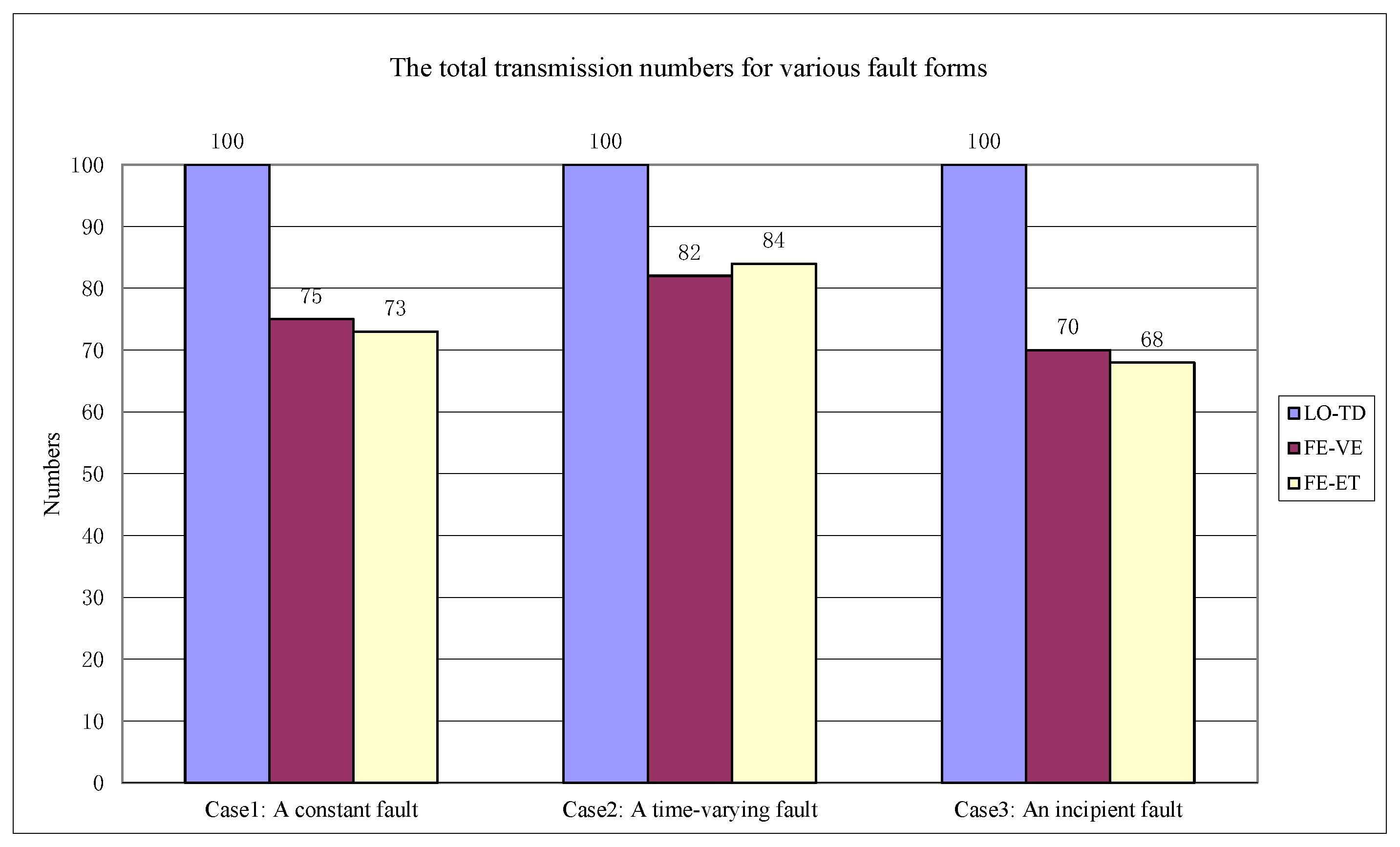
Figure 8. Compared with VE-FE, FE-ET designed using Theorem 1 not only offers superior rapidity of fault reconstruction but also achieves more accurate reconstruction of the various actuator fault scenarios. It can also be observed that both FE-ET and LO-TD demonstrate comparable rapidity and accuracy in fault reconstruction. However, the LO-TD algorithm shown in Figure 9 requires measurement information collected by wireless nodes at each time step to ensure accurate fault estimation. This can lead to a large amount of unnecessary data transmission in a fixed sampling interval, limiting the applicability of the LO-TD algorithm, especially for the considered CPSs in this study. In contrast, the advantage of FE-ET is the ability to adjust the data transmission interval to reduce the working time of wireless nodes and prolong the battery life. As a result, the proposed FE-ET algorithm can better meet the requirements of CPSs.
Furthermore, the total transmission numbers for the time-varying fault case in Figure 9 are relatively greater than for the other two fault cases. This is because the time-varying fault is characterized by high frequency, i.e., the upper bound of Δ f , k is greater than the upper bounds of the other two faults. As clearly evidenced in Figure 7, the designed FE-ET is unaffected by the time-varying fault feature. This further validates the designed event-triggered scheme, which is based on the result of Theorem 1. Its benefit is that data transmission occurs when the system state changes significantly or in emergency situations so that critical information cannot be missed.
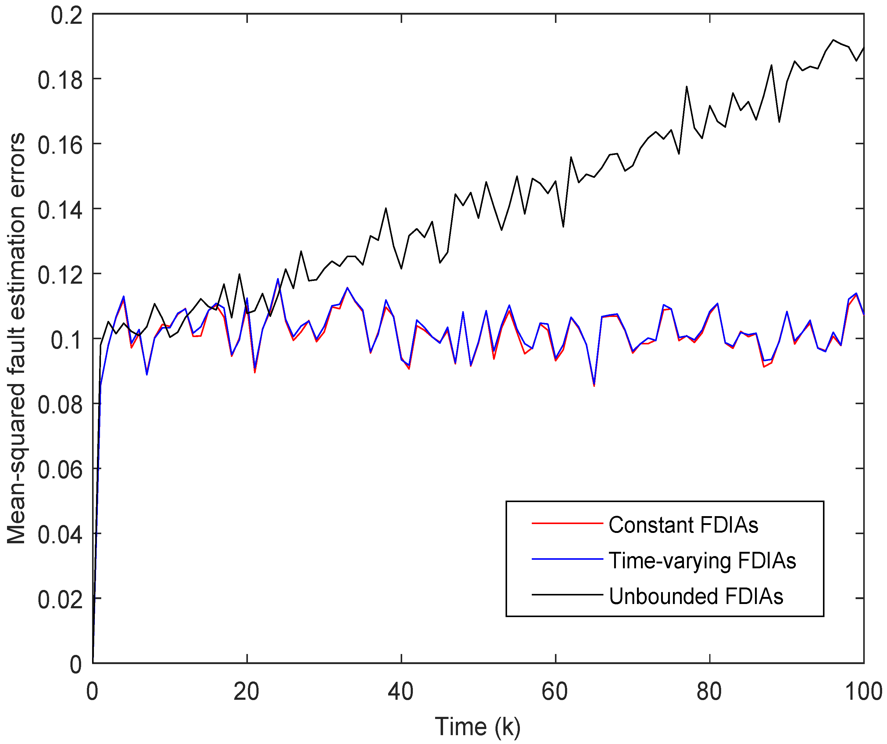
As illustrated in Experiment 1, different probabilities for FDIAs can lead to the different state estimation performance. In this experiment, the fault estimation performance is evaluated subject to different false information τ k sent by attackers. Constant false information, time-varying false information, and unbounded false information are respectively created as τ k = 0.3 , τ k = 0.3 sin 0.2 k and τ k = 0.3 e 0.2 k . The mean-squared fault estimation error curves are shown in Figure 10 with different deception attacks. As shown in Figure 10, the designed FE-ET demonstrates robustness against constant and time-varying false data injection launched by attackers. Under these two types of FDIAs, the fault estimation error can still converge to a small bound, indicating accurate fault reconstruction. This validates the robustness of FE-ET against certain levels of false data injection. Unfortunately, FE-ET loses its effectiveness in the face of unbounded false information. When the false information increases exponentially without any bound, the fault estimation error amplifies drastically, This renders FE-ET unable to accurately estimate fault, implying that the proposed FE-ET cannot cope with unbounded false information.
Experiment 3: Effectiveness and Robustness of Fault Tolerance
The final experiment evaluates the effectiveness of fault compensation based on the reconstructed time-varying fault in Figure 7. The system state responses under the fault-tolerant controller are shown in Figure 11 and Figure 12. The state responses using the estimated fault information perform well. It is clear that the fault estimator-based fault tolerant control strategy can effectively compensate for the impact of actuator faults on system performance. Similar to Experiment 1, the mean-squared state errors are examined in Figure 13 with different attack probabilities to ensure the security of the designed fault tolerant controller. Obviously, the mean-squared state errors rise slightly as the attack probability increases continuously.
All experiments demonstrate that the proposed fault estimator and fault tolerant controller can achieve satisfactory performance using the event-triggered transmission scheme. They show robustness against constant and time-varying false information, which are common FDIAs. Specifically, Experiment 1 verifies that the proposed estimator obtains accurate state estimation. Experiment 2 proves that the designed estimator accomplishes rapid and precise fault reconstruction for various fault scenarios. Experiment 3 indicates that the fault tolerant controller using the estimated information can effectively compensate for actuator faults. However, it should be noted that unbounded false information, which represents excessive FDIAs, has slightly negative impacts on the performance of the proposed algorithm. That is to say, the proposed fault estimator-based fault tolerance demonstrates effectiveness and robustness against FDIAs by implementing the event-triggered data transmission scheme in CPSs.

6. Conclusions

This study has proposed a systematic approach for the design of an event-triggered fault estimator and fault-tolerant controller for partial state-saturated CPSs with randomly occurring FDIAs. The reduced-order fault estimator is capable of simultaneously estimating system states and time-varying actuator faults with high accuracy. An event condition has been derived, and the corresponding event-triggered scheme has been developed to reduce sensor information transmission and energy consumption. Based on the separation property, stabilizing the fault-tolerant control using estimated information has been studied to ensure that the considered systems operate effectively, regardless of whether additional actuator faults appear or not. Utilizing the results of stochastic stability, sufficient conditions have been derived that restrict the influences of exogenous disturbances, fault signals, and false information sent by attackers. With the proposed event-triggered transmission scheme, the performance of the estimator-based fault-tolerant control has been guaranteed while significantly reducing the communication load, as demonstrated in the DC motor experiment.
However, we also find some open problems that should be solved in future research. One of them is the consideration of time-varying model parameters in the studied systems. In general CPSs, parameters often change over time due to factors such as environmental conditions, component wear, or other external disturbances. Moreover, incorporating domain knowledge, and integrating model-free methods with model-based approaches to create hybrid fault-tolerant control strategies may be an interesting direction for enhancing the effectiveness in various CPSs.

Author Contributions

In this work, Y.L. conceived and designed, performed, and analyzed the experiments and wrote the paper under the guidance of Y.W., W.Z. provided some suggestions on the background, introduction, and conclusion. All authors have read and agreed to the published version of the manuscript.

Funding

This work is supported by the Key University Science Research Project of Jiangsu Province under Grant 1020231350.

Conflicts of Interest

The authors declared no potential conflict of interest for the research, authorship, and/or publication of this article.

References

  1. Jiang, Y.; Yin, S. Recursive Total Principle Component Regression Based Fault Detection and Its Application to Vehicular Cyber-Physical Systems. IEEE Trans. Ind. Inform. 2018, 14, 1415–1423. [Google Scholar] [CrossRef]
  2. Jiang, Y.; Yin, S.; Kaynak, O. Performance Supervised Plant-Wide Process Monitoring in Industry 4.0: A Roadmap. IEEE Open J. Ind. Electron. Soc. 2021, 2, 21–35. [Google Scholar] [CrossRef]
  3. Jiang, Y.; Yin, S.; Dong, J.; Kaynak, O. A Review on Soft Sensors for Monitoring, Control, and Optimization of Industrial Processes. IEEE Sens. J. 2021, 21, 12868–12881. [Google Scholar] [CrossRef]
  4. Jia, Q.; Chen, W.; Zhang, Y.; Li, H. Fault Reconstruction and Fault-Tolerant Control via Learning Observers in Takagi–Sugeno Fuzzy Descriptor Systems With Time Delays. IEEE Trans. Ind. Electron. 2015, 62, 3885–3895. [Google Scholar] [CrossRef]
  5. Jiang, Y.; Yin, S.; Kaynak, O. Data-Driven Monitoring and Safety Control of Industrial Cyber-Physical Systems: Basics and Beyond. IEEE Access 2018, 6, 47374–47384. [Google Scholar] [CrossRef]
  6. Zhu, F.; Peng, L. Distributed adaptive event-triggered iterative learning controller based on a filtering network. Trans. Inst. Meas. Control 2021, 43, 3220–3232. [Google Scholar] [CrossRef]
  7. Li, Y.; Li, P.; Chen, W. An energy-efficient data transmission scheme for remote state estimation and applications to a water-tank system. ISA Trans. 2017, 70, 494–501. [Google Scholar] [CrossRef]
  8. Zhu, F.; Peng, L.; Yang, R. Event-triggered distributed filtering for Markov jump systems over sensor networks. Proc. Inst. Mech. Eng. Part I J. Syst. Control Eng. 2021, 235, 1482–1493. [Google Scholar] [CrossRef]
  9. Li, Y.; Peng, L. Event-triggered sensor data transmission policy for receding horizon recursive state estimation. J. Algorithms Comput. Technol. 2017, 11, 178–185. [Google Scholar] [CrossRef]
  10. Chen, H.; Shang, Y.; Sun, K. Multiple fault condition recognition of gearbox with sequential hypothesis test. Mech. Syst. Signal Process. 2013, 40, 469–482. [Google Scholar] [CrossRef]
  11. Chen, H.; Lu, Y.; Tu, L. Fault identification of gearbox degradation with optimized wavelet neural network. Shock Vib. 2013, 20, 247–262. [Google Scholar] [CrossRef]
  12. Liu, C.; Jiang, B.; Zhang, K.; Patton, R.J. Distributed fault-tolerant consensus tracking control of multi-agent systems under fixed and switching topologies. IEEE Trans. Circuits Syst. I Regul. Pap. 2021, 68, 1646–1658. [Google Scholar] [CrossRef]
  13. Yang, L.; Chen, H. Fault diagnosis of gearbox based on RBF-PF and particle swarm optimization wavelet neural network. Neural Comput. Appl. 2019, 31, 4463–4478. [Google Scholar] [CrossRef]
  14. Zhang, K.; Jiang, B.; Cocquempot, V. Distributed fault estimation observer design for multi-agent systems with switching topologies. IET Control Theory Appl. 2017, 11, 2801–2807. [Google Scholar] [CrossRef]
  15. Chen, H.; Huang, W.; Huang, J.; Cao, C.; Yang, L.; He, Y.; Zeng, L. Multi-fault condition monitoring of slurry pump with principle component analysis and sequential hypothesis test. Int. J. Pattern Recognit. Artif. Intell. 2020, 34, 2059019. [Google Scholar] [CrossRef]
  16. Chen, H.; Huang, L.; Yang, L.; Chen, Y.; Huang, J. Model-based method with nonlinear ultrasonic system identification for mechanical structural health assessment. Trans. Emerg. Telecommun. Technol. 2020, 31, e3955. [Google Scholar] [CrossRef]
  17. Chen, H.; Chen, Y.; Yang, L. Intelligent early structural health prognosis with nonlinear system identification for RFID signal analysis. Comput. Commun. 2020, 157, 150–161. [Google Scholar] [CrossRef]
  18. Chen, H.; Fan, D.; Huang, J.; Huang, W.; Zhang, G.; Huang, L. Finite element analysis model on ultrasonic phased array technique for material defect time of flight diffraction detection. Sci. Adv. Mater. 2020, 12, 665–675. [Google Scholar] [CrossRef]
  19. Hajshirmohamadi, S.; Davoodi, M.; Meskin, N.; Sheikholeslam, F. Event-triggered fault detection and isolation for discrete-time linear systems. IET Control Theory Appl. 2016, 10, 526–533. [Google Scholar] [CrossRef]
  20. Li, Y.; Peng, L. Event-triggered fault estimation for stochastic systems over multi-hop relay networks with randomly occurring sensor nonlinearities and packet dropouts. Sensors 2018, 18, 731. [Google Scholar] [CrossRef]
  21. Hu, L.; Wang, Z.; Han, Q.L.; Liu, X. Event-based input and state estimation for linear discrete time-varying systems. Int. J. Control 2018, 91, 101–113. [Google Scholar] [CrossRef]
  22. Yang, H.; Yin, S.; Han, H.; Sun, H. Sparse actuator and sensor attacks reconstruction for linear cyber-physical systems with sliding mode observer. IEEE Trans. Ind. Inform. 2021, 18, 3873–3884. [Google Scholar] [CrossRef]
  23. Yang, H.; Jiang, Y.; Yin, S. Adaptive Control for Cyber-Physical Systems against Actuator Attacks. In Proceedings of the 2020 IEEE Conference on Industrial Cyberphysical Systems (ICPS), Tampere, Finland, 10–12 June 2020; Volume 1, pp. 73–78. [Google Scholar]
  24. Wu, S.; Jiang, Y.; Luo, H.; Zhang, J.; Yin, S.; Kaynak, O. An integrated data-driven scheme for the defense of typical cyber–physical attacks. Reliab. Eng. Syst. Saf. 2022, 220, 108257. [Google Scholar] [CrossRef]
  25. Jiang, Y.; Wu, S.; Yang, H.; Luo, H.; Chen, Z.; Yin, S.; Kaynak, O. Secure data transmission and trustworthiness judgement approaches against cyber-physical attacks in an integrated data-driven framework. IEEE Trans. Syst. Man Cybern. Syst. 2022, 52, 7799–7809. [Google Scholar] [CrossRef]
  26. Jiang, Y.; Dong, J.; Yin, S. Improving the safety of distributed cyber-physical systems against false data injection attack by establishing interconnections. In Proceedings of the IECON 2020 The 46th Annual Conference of the IEEE Industrial Electronics Society, Singapore, 18–21 October 2020; pp. 2623–2628. [Google Scholar]
  27. Gao, Y.; Li, Y.; Peng, L. Event-triggered fault tolerant control for a class of state saturated systems subject to deception attacks. Trans. Inst. Meas. Control 2020, 42, 1935–1945. [Google Scholar] [CrossRef]
  28. Li, Y.; Wu, Q.; Peng, L. Simultaneous event-triggered fault detection and estimation for stochastic systems subject to deception attacks. Sensors 2018, 18, 321. [Google Scholar] [CrossRef]
  29. Huarong, Z.; Li, P.; Feifei, D. Data-driven Bipartite Consensus Control for Multi-agent Systems with Sensor Saturation. Inf. Control 2021, 50, 531–537. [Google Scholar]
  30. Ding, D.; Wang, Z.; Hu, J.; Shu, H. Dissipative control for state-saturated discrete time-varying systems with randomly occurring nonlinearities and missing measurements. Int. J. Control 2013, 86, 674–688. [Google Scholar] [CrossRef]
  31. Wen, J.; Peng, L.; Nguang, S. Stochastic finite-time boundedness on switching dynamics markovian jump linear systems with saturated and stochastic nonlinearities. Inf. Sci. 2016, 334, 65–82. [Google Scholar] [CrossRef]
  32. Liu, Q.; Wang, Z.; He, X.; Zhou, D. A survey of event-based strategies on control and estimation. Syst. Sci. Control Eng. Open Access J. 2014, 2, 90–97. [Google Scholar] [CrossRef]
  33. Li, Y.; Gao, Y.; Liu, Q.; Peng, L. Event-triggered fault estimation for stochastic state-delay systems against adversaries with application to a DC motor system. Int. J. Comput. Sci. Eng. 2020, 21, 325–333. [Google Scholar] [CrossRef]
  34. Chen, W.; Chen, W.T.; Saif, M.; Li, M.F.; Wu, H. Simultaneous fault isolation and estimation of lithium-ion batteries via synthesized design of Luenberger and learning observers. IEEE Trans. Control Syst. Technol. 2013, 22, 290–298. [Google Scholar] [CrossRef]
Figure 1. The physical connection diagram of the considered CPS.
Actuators 12 00197 g001
Figure 2. The physical connection diagram of the experimental platform.
Actuators 12 00197 g002
Figure 3. The mean-squared state estimation errors of system state 1.
Actuators 12 00197 g003
Figure 4. The mean-squared state estimation errors of system state 2.
Actuators 12 00197 g004
Figure 5. The mean-squared state estimation errors with different attack probabilities.
Actuators 12 00197 g005
Figure 6. Reconstruction of a suddenly changing constant fault.
Actuators 12 00197 g006
Figure 7. Reconstruction of a time-varying fault.
Actuators 12 00197 g007
Figure 8. Reconstruction of an incipient fault.
Actuators 12 00197 g008
Figure 9. The total transmission numbers for the time-varying fault case.
Actuators 12 00197 g009
Figure 10. The mean-squared fault estimation errors with different false information τ k .
Actuators 12 00197 g010
Figure 11. The state response curves of system state 1.
Actuators 12 00197 g011
Figure 12. The state response curves of system state 2.
Actuators 12 00197 g012
Figure 13. The mean-squared state errors with different attack probabilities.
Actuators 12 00197 g013
Disclaimer/Publisher’s Note: The statements, opinions and data contained in all publications are solely those of the individual author(s) and contributor(s) and not of MDPI and/or the editor(s). MDPI and/or the editor(s) disclaim responsibility for any injury to people or property resulting from any ideas, methods, instructions or products referred to in the content.

