1. Introduction
Recent developments in the field of robotics have led to the use of compliant actuators for providing a safe environment for humans and robots to interact. These actuators can be built with either passive compliance, using elastic components inside the actuators [
1], or active compliance [
2]. Passive compliance has been used in exoskeletons [
3], robotic hands [
4], and humanoid robots [
5], among other intrinsic compliance devices. Active compliance requires torque measurement at the robot joint along with designated control algorithms to simulate a compliant behaviour. Active compliance has been employed in recent works, including co-manipulation [
6], quadruped robots [
7], and pneumatic soft robots [
8].
While active compliance can be costly and complex, passive compliance is limited by difficulties in torque regulation and complex hardware design [
9,
10,
11]. An alternative approach to achieving compliant actuation is based on MR actuators (i.e., a serial combination of a motor and an MR clutch). This approach exploits the ability of MR fluid to change its viscosity on demand, hence the compliance of the actuator.
MR actuators have been used in robotics applications, including rehabilitation robots [
12], collaborative robots [
13], robot-assisted surgery [
14], as well as non-robotics applications, such as suspension systems in railway vehicles [
15], brakes [
16], and actuators [
17].
MR actuators have favorable characteristics, such as quick and reversible response, energy efficiency, and a high torque-to-weight ratio. Despite the advantages, controlling the transmission torque through an MR clutch (i.e., MR clutch output torque) without using external measurements remains a challenge due to the nonlinear [
18] and rate (frequency)-dependant [
19] hysteresis relationship between the input and output. One may use an F/T sensor to achieve closed-loop torque control. However, F/T torque sensors are known to have significant noise, which prohibits high-fidelity torque control. Moreover, this approach adds to the cost and complexity of the control system. To address these issues, we propose to use the magnetic flux density measured using embedded Hall sensors inside the MR clutch, along with a hysteresis model of the MR clutch, to achieve high-fidelity torque control [
20].
To this effect, we present a comparative study of six widely used hysteresis models and propose a computationally efficient but accurate algebraic model for hysteresis modeling and evaluate the results experimentally. Our goal is to obtain a computationally efficient model suitable for real-time torque control of rotary MR actuators. Our proposed approach does not require external F/T sensors and relies on Hall sensor measurements alone, which is substantially less expensive.
The contributions of this research are as follows:
Study of the magnetic hysteresis behaviour of rotary MR clutches.
Comparative analysis and experimental evaluation of six hysteresis models for predicting the output torque of an MR clutch using magnetic flux density measurements.
Proposing a computationally efficient and accurate torque estimation model for rotary MR clutches.
Evaluating the accuracy of model prediction and its applicability for real-time torque control.
The remainder of the paper is organized as follows: In
Section 2, several hysteresis models are introduced and categorized.
Section 3 introduces the structure and working principles of an MR clutch, and the experimental setup used for evaluating the results.
Section 4 presents four parametric hysteresis models, along with the modifications needed to adapt these models to an MR clutch.
Section 5 presents two non-parametric hysteresis modeling approaches.
Section 6 provides comparative analyses and validation results for the accuracy and generality of these models.
Section 7 concludes the paper.
2. Overview of Hysteresis Modeling in MR Clutches
Studies of MR actuators for robotic applications have identified the need for high-quality torque estimation models. In this regard, the estimation accuracy, robustness, and computational complexity of the models are among the considerations for selecting a suitable model. Existing models can be categorized as quasi-static and dynamic models. Dynamic models can be further divided into parametric and non-parametric models.
There have been several attempts to develop a quasi-static model of devices that uses MR fluids, but the rheology of the MR fluid can only be represented using the quasi-static analysis of the fluid flow in the flow mode [
21]. In these models, it is assumed that the MR fluid’s yield stress and viscosity are constant, which may not be the case in all applications under dynamic loads. As a result, the nonlinear behaviour of the device under dynamic loading, such as the rate-dependent hysteresis behaviour, is not accurately described using quasi-static models [
22].
Dynamic models can better predict the hysteretic behaviour of MR devices. A parametric dynamic model is normally presented using nonlinear ordinary differential equations with posteriori parameters. The posteriori parameters can be estimated by fitting the model response to measured outputs. Common models used are the Bingham, Herschel–Bulkley (H–B), Bouc–Wen (B–W), LuGre, hyperbolic tangent, and algebraic models.
The Bingham model can adequately characterize MR fluids, with the exception of nonlinear phenomena and shear thinning and/or thickening [
23]. Moreover, the model assumes that the viscosity of the fluid is constant below the yield stress [
24], making it difficult for the model to describe complex fluid behaviour. As a result, it fails to describe the roll-off phenomenon in MR devices at low force–velocity (i.e., change in magnetic flux density over time) in the hysteresis loop [
25]. The Bingham model can not accurately predict the rate-dependent hysteresis behaviour in MR devices. The H–B model is a more general model than the Bingham model, as it accounts for both shear thinning and thickening behaviours. The H–B model is simpler to use and less prone to overfitting than the Bingham model because it requires fitting fewer parameters. However, in the case of rotary disc-type MR clutches, the use of Bingham or H–B models makes it difficult to track the shape and location of the MR fluids yield surface, because of the non-uniform magnetic fields and varying gaps between the disks, leading to discontinuity and numerical issues [
26]. Due to the shortcomings of these models, we will not consider them in our subsequent analyses. We will provide a more in-depth study of the B–W, LuGre, hyperbolic tangent, and algebraic models in the following sections. These models vary in terms of their computational complexity and their ability to describe MR clutches hysteresis behaviour, including rate-dependency.
To provide a more comprehensive evaluation of different modeling approaches, and to determine the strengths and weaknesses of each approach related to our application, we will compare non-parametric models to the parametric models as well. Non-parametric dynamic models are entirely based on the analytical expressions obtained from experimental data. This means non-parametric models can capture ("learn") hysteresis behaviour from input-output data without having an explicit functional form. As such, the prediction accuracy of non-parametric models relies on the quality of input-output data. In our application, the input-output data are the responses of a prototype rotary MR clutch to various excitation conditions.
The commonly used models are the Hammerstein–Wiener (H–W) and nonlinear auto-regressive with eXogenous inputs (NARX) models. The NARX model is based on a neural network architecture that captures the dependencies between current and past inputs and outputs. In contrast, the H–W model does not take past inputs and outputs into account. Instead, it combines a linear dynamic system with static nonlinearities to represent the system, in which the nonlinear functions can be represented using various approaches, such as neural networks.
Some research groups have explored the use of a combination of non-parametric and parametric models to describe the asymmetric hysteresis behaviour observed in some cases [
27,
28]. MR clutches exhibit symmetric hysteresis behaviour for the most part; as such, it is not necessary to resort to such hybrid approaches in order to avoid the extra complexity of the model.
3. MR Clutch and Experimental Setup
In this section, we evaluate the performance of the parametric and non-parametric models introduced previously. We will use a prototype MR clutch and an experimental setup specifically designed for that purpose. The prototype MR clutch is shown in
Figure 1.
The prototype MR clutch used in our study is part of the actuation mechanism of the first joint of a 5-DOF compliant robot developed in [
13,
29]. The MR clutch consists of the rotor (input) and stator (output) disks, an electromagnetic coil, and embedded Hall sensors. The gaps between the rotor and stator disks are filled with MR fluid (LORD Corporation, MRF-140CG). The MR fluid generates shear forces between the rotor and stator disks that enable torque transmission through the MR clutch.
The experimental setup used to collect the data used in our study is shown in
Figure 2a. The components of the experimental setup are shown in
Figure 2b.
In this setup, the MR clutch input is coupled to a DC motor (Hacker, Q80-13XS) through a reduction gear. The DC motor provides mechanical power to the MR clutch at a constant angular velocity throughout the experiments. The output torque transmitted through the MR clutch is measured using a load cell (Transducer Techniques, SBO-500) fixed to the body of the setup. The output (transmitted) torques are measured for various sinusoidal excitations of the MR clutch with different frequencies. The commanded excitation signals are generated using MATLAB
Simulink through a dSPACE module (DS1103). The input excitation signals are applied to the MR clutch using a current driver (A-M-C, AZ12A8) for DC motors. The load cell and the embedded Hall effect sensors (Infineon, TLE4990) are also connected to the dSPACE using analog inputs. The Hall effect sensors are capable of measuring magnetic flux density with both polarities in either current direction. The data is collected at a sampling rate of 500 Hz for 30 s. After being filtered using a low-pass filter, the data is imported into MATLAB for model fitting.
Figure 3 depicts the output torque of the MR clutch versus the input magnetic flux density for a sinusoidal excitation of 0–3 A for four different frequencies.
4. Parametric Models of an MR Clutch
In this section, we will further analyze four parametric models to better understand the advantages and disadvantages of each model for real-time applications.
4.1. Bouc–Wen Model
The B–W hysteresis operator was first introduced by Bouc in 1971 [
30] to analytically describe hysteresis. It was then generalized by Wen in [
31]. This hysteresis operator was later introduced to model the hysteresis behaviour of an MR damper in [
32]. It then quickly gained popularity for modeling hysteresis in other MR devices due to its simplicity and generality. The damping force
F (N) in the B–W model is described as,
where
is the viscous coefficient,
is the stiffness coefficient,
is the scaling factor, and
x and
(mm) are the current and initial displacements, respectively. The value of
indicates the dissipation of energy inside the damper, but it does not affect the shape of the hysteresis loop significantly. On the other hand, a higher value of
results in a steeper slope of the hysteresis loop, which indicates a more viscous behaviour of the force with respect to displacement. The hysteresis variable
z can be expressed as,
in that
and
define the amplitude and shape of the hysteresis. Higher values of
and
lead to a narrower hysteresis loop.
affects the linearity of the hysteresis loop in the unloading region, and
n determines the smoothness of the transition from the pre-yield to post-yield region. A higher value of
n results in a sharper transition in the hysteresis loop.
To adapt this model to an MR clutch, the magnetic flux density and its derivative are used as the inputs to the model. The modified model can be written as,
where
T (N·m) is the estimated torque, and
B (mT) is the magnetic flux density measured by the Hall effect sensor. The hysteresis variable z is expressed as,
In our proposed model for an MR clutch, the variable
n is set to 1 since no transitions from the pre-yield to the post-yield region are observed in the graphs depicted in
Figure 3. In this model, the coefficients
c and
k represent the viscosity and stiffness of the MR clutch as in the original B–W model. The rest of the parameters are the same as the original model and can be determined in MATLAB through offline parameter estimation.
4.2. LuGre Model
The LuGre model was first proposed by De Wit et al. [
33] for simulating the friction dynamics, and it was first presented to represent the dynamics of an MR damper at the 15th IFAC World Congress [
34]. Later, the model was further modified in [
35] to reflect the dynamics of MR dampers. The model is expressed as,
where
are parameters related to the shape and scale of the hysteresis loops.
c and
k denote the viscous and stiffness coefficients of the MR damper,
x (mm) is the displacement and
F (N) is the damping force. In the original LuGre model,
z is an internal state that represents the average deflection of some fictitious bristles that cause friction between the two surfaces. In this model, two modes, including pre-sliding and sliding modes, are assumed and the viscous and stiffness parameters in the model describe the behaviour of these imaginary bristles during the pre-sliding mode. It is difficult to provide a similar interpretation for such parameters in relation to MR fluids. One can imagine the internal state
z as the deformation of the micro-structure columns formed in the MR fluid. The changes in variable
z are governed by the following nonlinear dynamics,
To adapt the LuGre model to an MR clutch, similar changes are made. The adapted LuGre model for an MR clutch is expressed as,
where
in that
B (mT) is the magnetic flux density measured by the Hall effect sensor,
(N·m) is the residual torque, and all other parameters are as defined in the original LuGre model.
4.3. Hyperbolic Tangent Model
The hyperbolic tangent model has been used to model various systems with hysteresis, including smart actuators [
36], power transformers [
37], and MR devices. The model was first proposed in [
38] to describe the force–velocity characteristics of an MR damper with hysteresis. The model is given by,
where
c and
k are the viscous and stiffness coefficients,
is the scaling factor of the hysteresis variable
z,
x (mm) is the damper displacement, and
(N) is the damper initial force. The changes in the hysteresis variable are described as,
in that
and
are the parameters to shape the hysteresis loop. In contrast to the two previous models, the hyperbolic tangent model is not formulated using dynamic equations, which lessens the computational complexity of this model.
To help visualize the effect of different parameters in this model,
Figure 4 depicts the change in the shape of the hysteresis loop with respect to each parameter.
In this figure, the stiffness is represented by k, which defines the slope of the hysteresis, and the product determines the inclination of the hysteresis loop, shown with the dotted blue line in the figure. This line grows to a small hysteresis loop shown in red after increasing the shape factors c. The loop expands to a black medium hysteresis with the increase in . The scale factor determines the of the hysteresis. The hysteresis variable z is scaled by to adjust the of the hysteresis loop, and, together with , determines the location of the loop along the vertical axis. The final hysteresis loop is depicted in purple.
The hyperbolic tangent model is once again adapted to the MR clutch. The MR clutch hyperbolic tangent model can be expressed as,
where
in that
T (N·m) is the estimated torque,
(N·m) is the initial torque,
B (mT) is the magnetic flux density measured by the Hall effect sensor, and the remaining parameters are as defined for the original hyperbolic model.
4.4. Algebraic Model
Different from the Bouc–Wen and LuGre models, the algebraic model describes the hysteresis behaviour using a simple mathematical formulation and without the use of an internal state variable. This model is computationally much more efficient, making it more suitable for real-time embedded controllers.
The model combines the rubber’s visco-elastic effect and the strain stiffening effect due to the model input. This model was originally developed for an MR elastomer in [
39]. The model can be represented as,
where
c and
k denote the damping and stiffness coefficients,
is a coefficient for the power law element,
(N) is the initial force, and
x (mm) is the displacement.
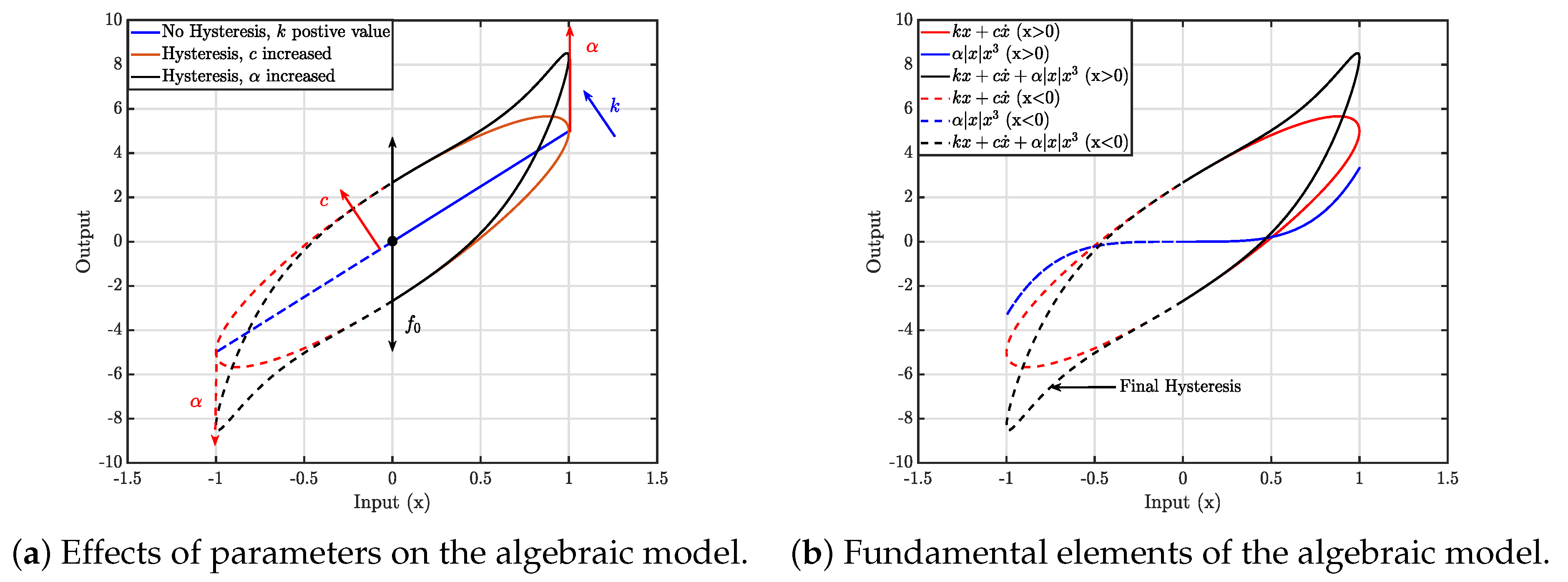
Figure 5a illustrates the effects of the model parameters on the shape of the hysteresis loop. The stiffness coefficient
k represents the inclination of the hysteresis loop, while the damping coefficient
c and the coefficient of the power law element
change the shape of the hysteresis loop. As can be seen, the size of the hysteresis loop grows with increase in
c and
.
Figure 5b illustrates the combination of the two effects, namely, the visco-elastic effect
, shown with a dotted blue line, and the strain stiffening effect
, shown with a solid red line with circle. The combination of these two phenomena results in the hysteresis loop shown by the solid black line.
The algebraic adapted model to an MR clutch can be expressed as,
where
B (mT) is the magnetic flux density. The absolute value in the equation is designed to account for both the positive and negative magnetic flux density, which depends on the direction of current applied to the MR clutch.
T and
are the estimated and initial torques, respectively, and other parameters are as defined in the original model.
The intricate nature of the molecular interactions that underlie the behaviour of MR fluids poses a challenge for providing a comprehensive interpretation of how each model parameter affects the physical behaviour of these fluids. Conducting a thorough analysis of MR fluid behaviour is beyond the scope of this study. Instead, we adopt a more pragmatic approach by demonstrating how these parameters impact the shape of the hysteresis loop, without delving into theoretical details.
5. Non-Parametric Models of an MR Clutch
The non-parametric models will be introduced and described in this section. These models are typically derived from a large amount of experimental data through analytical methods. These models often do not require knowledge and pre-defined mathematical formulation a priori, as they are fundamentally unrelated to physical phenomenon that they describe. This is advantageous when modeling complex systems, where the underlying physical mechanisms are too complex to be modeled accurately using traditional physics-based models. In other words, they are easier to adapt to the data with a desired fitting accuracy.
5.1. Hammerstein–Wiener Model
The Hammerstein–Wiener (H–W) model has been utilized to model systems with backlash [
40] and hysteresis [
41]. This model can be separated into the Hammerstein model, in which a static nonlinear block connects to a linear dynamic block in series, and the Wiener model, in which a linear dynamic block connects to a static nonlinear block. Combining the two separate models results in the H–W model. The block diagram of an H–W model is shown in
Figure 6, which consists of two static nonlinear functions and a linear transfer function. The linear dynamic block represents the transfer function that maps the output torque of the MR clutch to changes in the input current (or the magnetic flux density). The Hammerstein block represents the magnetization dynamics of the MR clutch relating the magnetic field to the output torque. The Wiener block represents the hysteresis behaviour caused by residual magnetization of the ferromagnetic materials after the magnetic field is weakened or reversed. This is because the residual magnetization can cause the MR fluid to maintain a certain degree of viscosity, leading to a residual torque.
The mathematical expression of the H–W model is given by,
and
where (
15) is the Hammerstein nonlinear mapping function
H that transforms input magnetic flux density
to
, (
16) is the linear transfer function
L that transforms
to
, and (
17) is the Wiener nonlinear mapping function
W that maps
to the model output torque
. The outputs of both nonlinear functions are solely dependent on the input value at the specified time
t, not on the values from earlier points in time. Configuring this model using the MATLAB System Identification Toolbox™ enables selection of the nonlinear function, including piecewise, wavelet network, sigmoid network, unit gain, etc. Typically, the selection of the functions and the corresponding parameters are determined by trial and error. In this work, both nonlinear blocks were selected as wavelet networks because of their superior performance in dealing with non-stationary signals with a nonlinear transient. The details of configuring the H–W model will be described in
Section 6.
5.2. Nonlinear ARX Model
The Nonlinear AutoRegressive with eXogenous inputs (NARX) model can predict the output of a system for a given input, based on a trained neural network that incorporates the past input and output data [
42], as well as other eXogenous inputs, such as disturbance. The model is frequently used to model MR dampers and clutches [
43,
44] in the fields of robotics, civil engineering, automotive engineering. Compared to the H–W model, the NARX model takes into account the past inputs and outputs to determine the dependencies (nonlinear hysteresis) between them. The model makes more accurate predictions based on the current input. The block diagram of the model is presented in
Figure 7.
As shown, the model consists of past inputs and outputs, a mapping function, and a feedback connection, which allows the model output to be fed back to relearn from its own prediction. In addition, the model also considers the time delay, which refers to the number of time steps between the input and output data that are used to train the model. The nonlinear mapping function
is expressed as,
where
is a nonlinear mapping function that maps the current input, and past inputs and outputs to the output at time
t. The inputs to the
function include,
, the fed-back term,
, the current model input, and
, the past inputs to the model. The activation function of
f can be chosen from wavelet networks, tree partition networks, sigmoid networks, etc., to adapt to various systems. In this work, the activation function is configured as wavelet networks. This is because a wavelet network can adapt to the varying hysteresis behaviour by adjusting its coefficients and functions, leading to better estimation accuracy. The details of configuring a NARX model will be described in
Section 6.
In addition to the nonlinear mapping function that captures the local nonlinear behaviour, the linear mapping function
L is needed to capture the global linear relationship between inputs and outputs. It also provides an estimation baseline for the nonlinear mapping function, which makes it easier to interpret the hysteresis behaviour. It can be expressed as,
where the inputs to
L are the same as the nonlinear mapping function and
to
are the weights for the inputs. The weights are updated during the training process. Finally, the linear and nonlinear mapping functions are combined with an offset term to produce the model output
.
6. Model Comparisons
The previous sections introduced and discussed six hysteresis models. To further investigate and focus on obtaining an accurate and computationally efficient hysteresis model for rotary MR clutches, we will train the models using the magnetic flux density and the output torque of a prototype MR clutch. The results of the model fitting are compared and evaluated in
Section 6.1. In addition, the parameters, fitting time, execution time, and stack size are recorded and analyzed to help select the optimal model.
Section 6.2 compares and validates the selected algebraic model through experimental validations.
For model fitting, the Simulink Parameter Estimation Function (PEF) is used to estimate the parameters of the parametric models. The MATLAB System Identification Toolbox™ (SIT)’s nonlinear model tool is used to create the non-parametric models. For the former method, the cost function is set to sum of squares error (SSE), and the optimization method is set to nonlinear least square (NLS). In the latter method, the linear block of the H–W model is configured with two zeros, five poles, and one time unit of input delay. The two nonlinear blocks used in this model are the wavelet network with automatic selection of the number of wavelets. This means the number of parameters will be based on the finest fitting accuracy, which can lead to excessive use of parameters.
The input block of the NARX model consists of six time units of past inputs and one time unit of past output. The nonlinear mapping function employed in this model is the wavelet network, which automatically selects the number of wavelets. Similarly to the H–W model, the number of parameters is also automatically selected based on the finest fitting accuracy.
6.1. Model Fitting
In this section, we will present a series of experiments to obtain the data related to the dynamic response of the MR clutch. These experiments were designed to provide comprehensive datasets for training the hysteresis models. The inputs were sinusoidal current excitation signals with amplitude ranging from 0 to 3 A and frequencies between 1 Hz and 9 Hz with an interval of 2 Hz. The experimental data were filtered by a low-pass filter before being used in PEF and SIT for data fitting. The fitting results are presented in
Figure 8. The fitting errors are depicted as box plots in the same figure, which represent the distribution and spread of errors across different models.
To make a quantitative comparison among the fitting results, the relative root mean square error (R-RMSE) was used to compare the accuracy of various models, where a lower value indicates a more accurate model. The R-RMSE is obtained as,
where
represents the
ith measured torque in the total of
N data points, and
stands for the corresponding model estimated value. In
Table 1, the R-RMSE values for six models for five different frequencies are listed.
Table 2 provides insight into the computational complexity of the models based on metrics obtained using a PC with an Intel
® Core™ i5-4200H CPU @ 2.8 GHz processor and 16 GB of RAM. The execution time and stack size were obtained through the Performance Advisor and Static Code Metrics function of MATLAB Embedded Coder
.
Table 1 shows that, for all models, the fitting accuracy decreases slightly as the frequency of excitation increases. Overall the hyperbolic tangent and algebraic models demonstrate better fitting accuracy across all frequencies than the B–W and LuGre models. Comparing non-parametric and parametric model performances, the non-parametric models show marginally better fitting accuracy.
Table 2 provides a comprehensive evaluation of the computational burden of these models by comparing the number of required parameters, fitting time, execution time, and stack size for different models. The four parametric models exhibit a relatively small difference in terms of the required stack size that ranges from 96 bytes to 192 bytes. The execution time for these models exhibits a similar trend, with the hyperbolic tangent and algebraic models having the shortest execution times among the four models. Moreover, the algebraic model requires the least time for fitting the experimental data. The fitting time becomes an important consideration in adaptive modeling approaches. In contrast, the non-parametric models require a significantly larger amount of parameters to achieve slightly more accurate fitting results. However, the required stack sizes for these models are approximately 15 to 28 times larger than those of the algebraic model. The non-parametric models also take two to three times longer than the algebraic model to execute on the same PC configuration mentioned above. If executed on an embedded computer with limited internal memories and computational bandwidth, these results are expected to be exacerbated. Considering these results, the hyperbolic tangent and algebraic models are further evaluated for selecting the most suitable model. In the following, we will further compare parametric models in terms of their fitted parameters.
The fitted parameters of parametric models are listed in
Table 3,
Table 4,
Table 5 and
Table 6. In these tables, standard deviation (SD) values are calculated to quantify the extent to which the values of model parameters vary across different frequencies. This indicator is important to identify the model with more prediction robustness and accuracy over a wider range of frequencies.
In light of this fact, we note that the parameters of the algebraic model have the smallest SD values among all four parametric models. This suggests that the algebraic model can provide more accurate estimation results over a wider range of frequencies and the model should exhibit more generality. In comparison, the other three models have much larger SD values, which results in difficulty in accurately estimating the output torque.
In addition to analyzing the SD values of the parameters, we also observed the presence of negative values among them. The interpretation of negative parameters can vary depending on the specific model under consideration. For example, in the B–W and LuGre models, a negative damping coefficient may indicate that the system is dissipative, whereas a negative stiffness coefficient may suggest instability. Conversely, negative parameter values in the hyperbolic tangent and algebraic models may not necessarily have a physical interpretation and may instead be a byproduct of the parameter identification algorithm.
It is important to carefully consider the meaning of negative parameter values in different models, as they can have different implications for the behaviour and stability of the system. However, in cases where the negative values are not physically meaningful, it is crucial to be aware of their potential origins and to take them into account when interpreting the results of the parameter identification process.
6.2. Model Validation
In this section, we will experimentally evaluate the accuracy and the generality of the six models. To this effect, a multi-sine as well as a swept-sine signal were applied to the MR clutch. The output torque of the MR clutch was recorded for a duration of 40 s. The results were then compared with those from each model.
The values of the parameters for the parametric models were obtained as the average value of each parameter for five different frequencies, as listed in
Table 3,
Table 4,
Table 5 and
Table 6. For the non-parametric models, we used the values of the parameters obtained for the 5 Hz dataset fitted to these models.
The multi-sine signal was constructed as,
where
and
,
are the magnitudes and frequencies of different sinusoidal waves. The multi-sine excitation signal is the sum of 11 sinusoidal waves with uniformly selected frequencies within the range of 1 Hz to 10 Hz and different magnitudes.
The swept-sine signal was constructed as,
where
are the magnitude, start frequency, stop frequency, signal duration, and offset values, respectively. The magnitude of the swept-sine signal was chosen to match the fitting process (0-3 A), and its frequency was set to change from 0.1 Hz to 5 Hz.
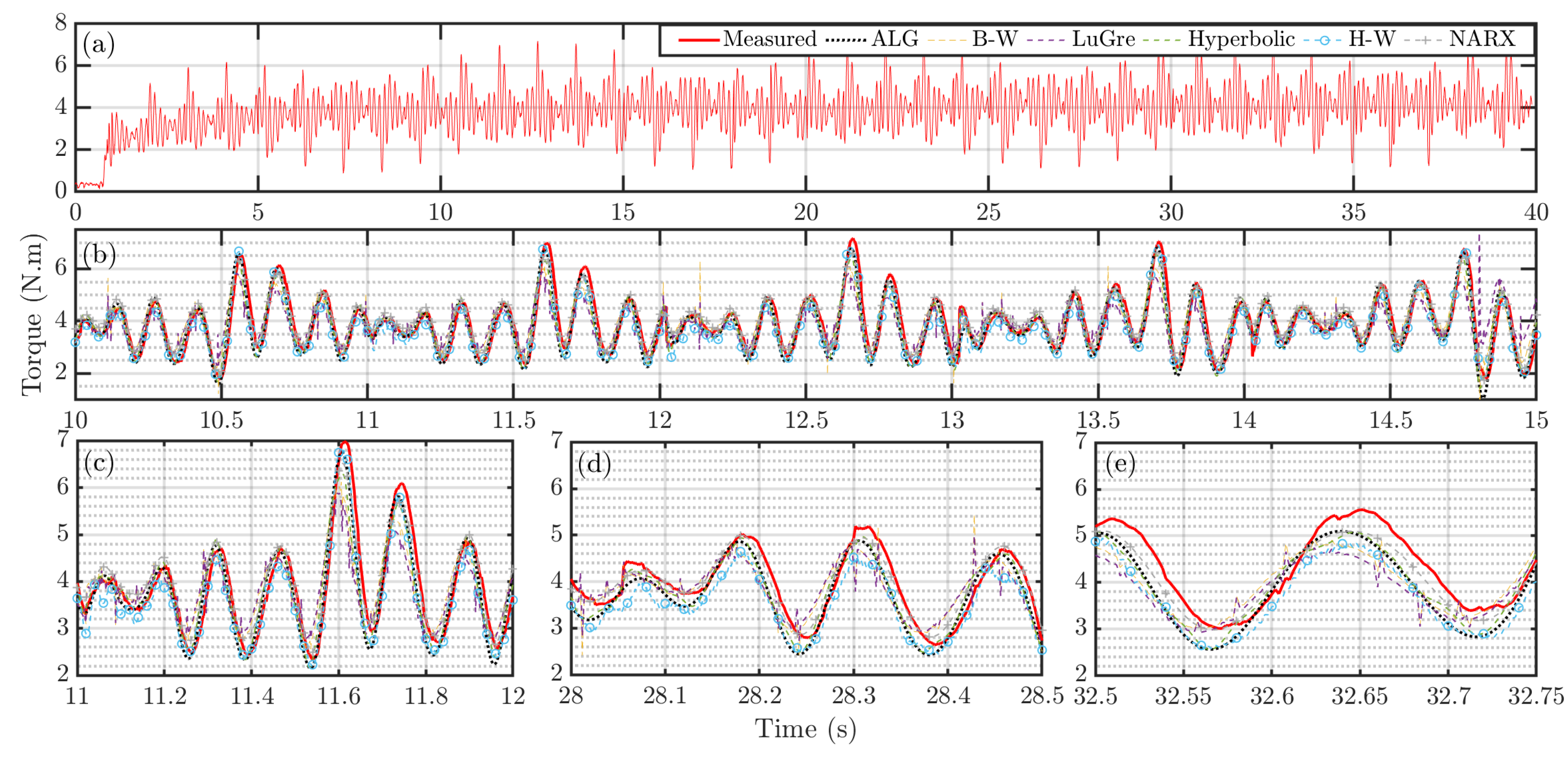
Figure 9 and
Figure 10 show the measured torque and estimated output torques for the multi-sine and swept-sine signals, respectively.
To further analyze the accuracy of the model prediction results, both R-RMSE and the coefficient of determination (
) index were used to provide a comprehensive evaluation of the model validation results. The latter metric can evaluate the overall goodness of the fitting between the predicted and measured data points.
is calculated as the sum of squares errors to the total sum of squares. A high
value indicates that the model explains a large proportion of the variation in the data, while a low
value suggests that the model does not fit to the data well. It can be expressed as,
where
represents the
ith measured torque in the total of
N data points,
stands for the corresponding model estimated value, and
is the mean value of the measured torque. The results for R-RMSE and
are shown in
Table 7.
Among the four parametric models, the algebraic model has the lowest R-RMSE values of 9.0% and 11.7% for the multi-sine and swept-sine signals, respectively. The algebraic model also has the highest values of 0.868 and 0.945 for these two signals. When comparing all models, the algebraic model still outperforms the H–W model but is not as accurate as the NARX model, which has R-RMSE values of 7.96% and 8.08%, and values of and for the two input signals. The result implies that the algebraic model and the NARX model can both provide more accurate estimation than the other four models. However, as shown previously, the NARX model has much higher memory requirements (up to 28 times more) and higher computational time (up to 3 times more). These drawbacks pose implementation challenges for embedded computers.
Looking at the overall results, it is seen that the R-RMSE values for swept-sine are higher than those for multi-sine, suggesting that the models estimate better for the multi-sine signal. However, the values show the opposite. This indicates that the models are able to estimate the overall shape of the swept-sine signal more accurately, except for higher frequencies where the models have a larger phase shift, resulting in less accurate predictions.
7. Conclusions
In this study, the frequency-dependent magnetic hysteresis present in a prototype rotary MR clutch was investigated. Six hysteresis models, including four parametric and two non-parametric models, were experimentally studied and compared. The models utilized magnetic flux density measurements as input to predict the output torque of the MR clutch. The performance of the models was compared based on the R-RMSE and values for model predictions, as well as the computational requirements of the models.
The results showed that the algebraic hysteresis model offered the best computational efficiency with good estimation accuracy among all parametric and non-parametric models. It was found that the algebraic model required 28 times less memory and computed 3 times faster than the non-parametric models. These results are important for selecting a suitable model for real-time applications in embedded computers.
Overall, this study provided valuable insights into the frequency-dependent magnetic hysteresis of rotary MR clutches and offered a practical solution for torque control using the algebraic hysteresis model. The findings could be useful for designing more efficient and effective robotic systems that require precise torque control.


