1. Introduction
In recent years, with the rapid development of modern industry, traditional factories have gradually merged with intelligent factories. As a result, unmanned forklifts have been widely implemented for in-plant logistics [
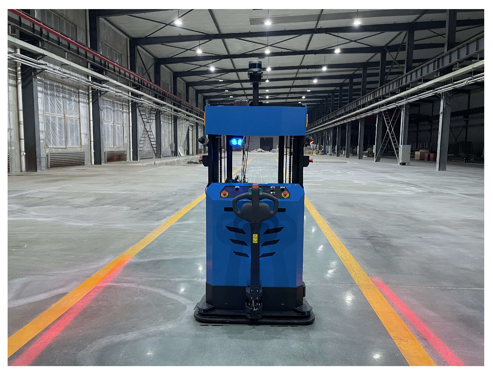
1]. An unmanned forklift in a factory is shown in
Figure 1.
At present, the navigational solutions of industrial unmanned forklifts can only accomplish the automatic navigation of fixed routes, and all the operational tracks are generated offline [
2]. If the navigation area changes, the navigation route has to be adjusted, and redeploying the whole navigation system presents a time-consuming, inflexible, and costly procedure. This inflexible deployment mode significantly limits the application of the system.
Therefore, current unmanned forklifts all operate on pre-designed fixed routes. When they arrive at the handling point, they usually employ the “blind fork” method to complete their task. If these forklifts deviate from the fixed routing, these forklifts are unable to fulfill their mission. Furthermore, they have also occasionally caused serious accidents [
3]. In this off-line path generation method, even if the deviation of the final posture can be detected by the sensor, it is challenging for the vehicle controller to correct the deviation within a relatively short distance. Therefore, it is difficult for current unmanned forklifts to meet the handling requirements of flexible production required at an industrial scale, which significantly limits the application of unmanned forklifts in intelligent digital factories.
This study focuses on the precise flexible online trajectory planning of industrial unmanned forklifts. In order to solve issues regarding the inflexible deployment of the forklift navigation system and overcome the limitations of flexible online trajectory planning in modern factories, we proposed and evaluated a precise flexible online trajectory planner for industrial forklifts. The proposal can be used for online motion planning of car-like vehicles regardless of the end-pose. In this method, the original path output of the motion planner based on sampling is used to smooth the path based on optimization, which can then achieve a smooth and collision-free trajectory online and improve the pose accuracy at the end of the trajectory.
This study contributed the following innovations: (1) We proposed a new path smoothing approach based on a two-step method that can be used in a complete online navigation system to plan high-precision driving trajectories for car-like vehicles. Firstly, a feasible primitive path was found, and then the optimal control function was constructed. The security envelope of each point in the primitive path, the kinematics constraints, the dynamics constraints, and the turning constraint at the end of the path were used as the constraint conditions of the objective function, and the path smoothing was carried out using an optimization method. This method not only effectively improved the accuracy of path planning, but also eliminated the additional curvature and collision safety reviews typically required after path smoothing, improving the efficiency and safety of path planning. (2) A new, rapid calculation method of a spatial security envelope was proposed. These safety envelopes added the attitude and angle constraints of the vehicle while considering the positional collision avoidance constraints, which limited the search space of the robot to a collision-free state.Firstly, an off-line calculation method was used to pre-calculate the spatial safety envelope set of the vehicle according to the forklift model. The envelope set considered both the area of the polygon envelope and the range of the rotation angle. It then generated a lookup table (PC: polygon constraint) of the envelope set via the weight relationships. Secondly, based on the collision-free path
(which satisfied the kinematic constraints) output by the lattice motion planner, each waypoint in the path was generated in a spatial security envelope, and finally the spatial security envelope around the whole path was obtained. See
Appendix A for details of the summary of the variable comparison table.
2. Related Work
At present, unmanned forklifts used in factories operate according to predefined trajectories, which are typically generated by manual definitions or manually by operators [
4]. Although these methods are simple in principle, the trajectories generated by these methods bear issues that warrant being addressed. These include their high deployment costs and lack of flexibility in adapting to environmental alterations in factory settings, such as adding goods to assembly points or modifying distribution routes in warehouses. To resolve such problems, a new trajectory planner is required for the flexible online trajectory generation of industrial forklifts.
At present, researchers have suggested numerous motion-planning methods. Motion planning is usually divided into two categories: front-end path search and back-end path optimization. The front-end path search is responsible for identifying a safe and collision-free path on the map, and then the back-end path optimization considers the kinematics, dynamics, and environmental factors of vehicles as constraints; optimizes the waypoints on the initial path in terms of smoothness and safety; and then generates a smooth path. Therefore, the motion-planning method combining a front-end path search with a back-end path optimization has become the standard in motion planning.
The following provides a detailed introduction to the literature on related topics. The existing front-end path-search methods for industrial unmanned forklifts include graph-based search methods and sampling-based methods. These methods usually discretize the continuous state space into a node graph and then search for effective links from the starting node to the target node in the graph. Path search methods based on graph search mainly include A* [
5,
6], Dijkstra [
7], and so on. The path-search method based on sampling is divided into two steps, namely, sampling the state space and the control space. Typical methods for sampling a state space include the state lattice method [
8,
9] and rapidly exploring random-tree sequence [
10,
11]. Therefore, typical control space sampling methods have included the hybrid A algorithm [
12] and dynamic window method [
13]. Specifically, Dang et al. [
12] suggested the hybrid A-star algorithm, which combined front-end searching with a vehicle kinematics model, and considered vehicle kinematics constraints while searching. Subsequently, this not only improved search efficiency but also satisfied the vehicle model with an under-actuated structure, such as a forklift truck. It was used to solve the vehicle planning problem in parking lots, U-turns, and other scenarios. However, the path searched by this kind of algorithm was not an optimal path in terms of vehicle kinematics constraints. Therefore, during the search process, the algorithm only focused on a localized optimal solution, rather than a global optimal solution. Pivtoraiko and Kelly [
14] suggested the concept of the state lattice search, which was used to build an efficient dynamic motion planner. However, the algorithm state lattice search was very expensive and difficult to build online. Therefore, the path generated by this method had the disadvantage of a discontinuous state space, which failed to meet the high-precision parking demands when used alone.
Back-end path optimization is divided into special curve-smoothing methods and optimization methods [
15]. (1) The special curve-smoothing method employs the waypoint obtained by the path search [
16,
17] as input, and then uses a special curve to generate a feasible smooth path. Commonly used curves have included the Dubins curve [
18], the Bezier curve [
19], the B-spline curve, and so on. It was necessary to change the original path by using the above special curve method directly, which the collision-free path could not guarantee. Therefore, an extra processing step was required to determine whether the path in the new representation was still conflict-free. This proved to be time-consuming and negatively affected the speed of online solutions. (2) The trajectory planning task was described as an optimal control problem (OCP) based on an optimization method, and was discretized into a nonlinear-programming (NLP) problem [
20]. Functional optimization method obtained smooth paths by minimizing constraints such as velocity, acceleration, and jerk. Zhu et al. [
21] proposed a trajectory-smoothing method based on convex optimization, which was used for trajectory smoothing and speed optimization of mobile robots with similar automobile dynamics. In addition, Choi et al. [
22] proposed a path-planning algorithm for non-holonomic, constrained vehicles operating in a semi-structured environment. Sprunk et al. [
23] considered the smoothness of the path while ignoring security constraints during optimization; therefore, it was necessary to evaluate the security after optimization.
Others have used security envelope constraints during path optimization, which limited the movement range of each waypoint. However, the security envelope was of the same size and lacked flexibility [
24]. Furthermore, the authors of [
25] used a variable-sized safety envelope, that is, the size of the safety envelope was dynamically generated according to the distance between the vehicle model and the obstacle. However, this method did not consider the rotation angle of the vehicle on the safety envelope, especially for a vehicle body with an under-driven structure, such as a forklift, for which the angle constraint was equally important. In summary, the extraction of safety envelopes has proven to be a time-consuming process. To achieve online path generation, rapid path-safety-envelope extraction is critical.
This study provided various insights.First, we used the anytime repairing A* (ARA*) algorithm to search a collision-free feasible path under finite time constraints. This method ensured that the reference trajectory could be quickly obtained within a finite time period. The state grid map was reasonably constructed according to the real-time positioning and orientation of the forklifts. Second, a path-smoothing method was proposed based on optimizations including the safety envelope, rotation angle constraints, kinematics, and dynamics constraints. This method directly added state-space constraints during the smoothing process, which eliminated a second verification step after smoothing. Third, since the generation of the secure envelope has been problematic due to being time-consuming and inflexible, we designed a rapid and secure envelope extraction method that considered both positioning and angle constraints. Lastly, using the B-spline curve method, the optimized path was guided by time parameters to ensure a safe and smooth trajectory that met the kinematics and dynamics constraints. In the experiment, the industrial unmanned forklifts using the flexible online trajectory planner proposed in this paper generated smooth, drivable trajectories for any target pose within a few seconds.
3. Methodology
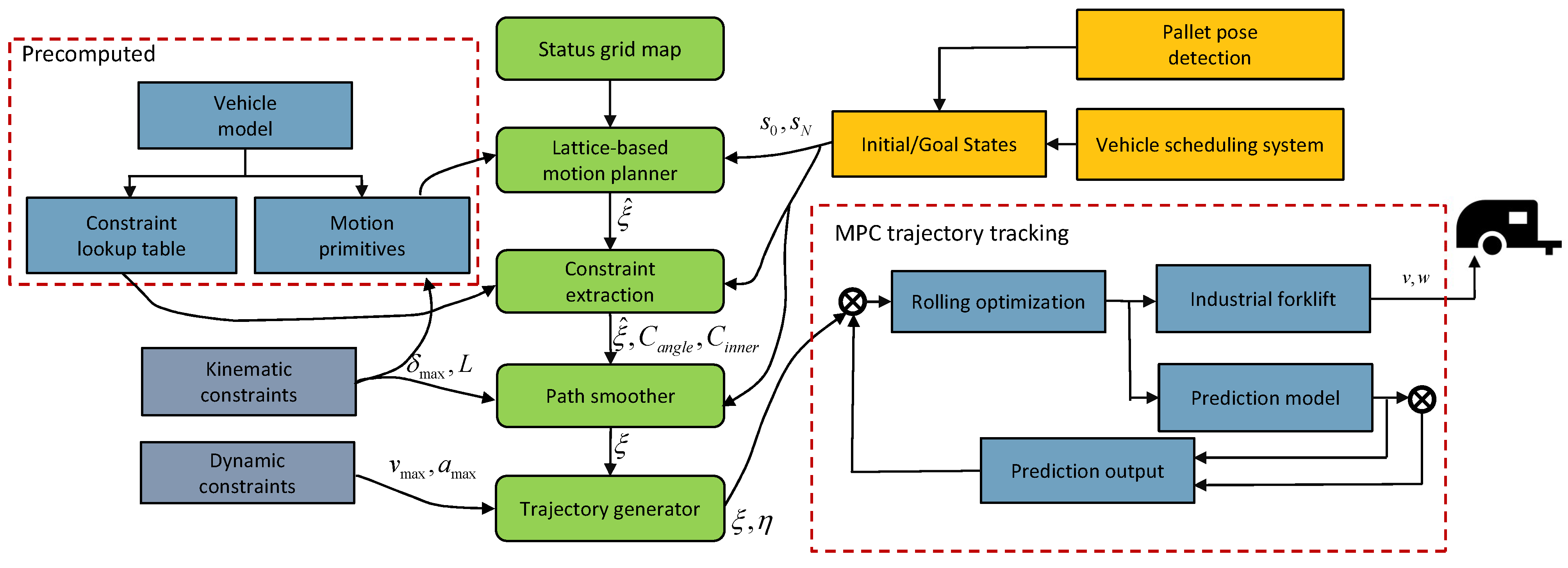
This paper focused on the development of high-precision flexible online trajectory planning for industrial unmanned forklifts. A motion planning algorithm was proposed based on optimization. We used a five-step method, as shown in
Figure 2.
First, we used the lattice-based motion planner to calculate the trajectory path that would satisfy the forklift kinematics constraint, which was the basis of the path constraint step. Second, we pre-calculated the safety envelope set of the vehicle offline, according to the forklift model, and used the offline method to calculate the envelope set to improve the efficiency of the trajectory optimization steps. Next, we extracted the free-space envelope around the path according to the original path and the calculated space envelope set, and expressed it in the form of a convex polyhedron constraint of the vehicle state. The path space envelope generated in this step was used as a security constraint item for the subsequent path-smoothing step. The path-smoothing based on the optimization method proposed in this paper was then used to address the path and the corresponding constraints, and a collision-free continuous path was obtained. Finally, the trajectory generator used a B-spline interpolation method to generate a safe and smooth trajectory that satisfied the dynamic and time constraints. A model-based predictive control algorithm was used to track the generated trajectory with high precision. Since this study focused on safety envelope extraction and path optimization, the additional details in
Figure 2 are briefly described for the completeness of the algorithm description.
3.1. Establishment of a Kinematic Model of the Forklift Truck
Because of the low speed of forklifts in logistics transportation, the lateral forces of forklifts are low. Assuming that the forklift would not skid during operation, we only needed to establish the forklift kinematic model to complete the trajectory planner design. Assuming that the forklift body was rigid and the deformation of wheels could be ignored, the forklift motion would not pitch or roll on the plane, and the contact point between the wheels and the ground would only produce rolling contact without sliding. The kinematic model of the forklift is shown in
Figure 3.
In
Figure 3, XOY is the world coordinate system;
represents the forklift front-wheel coordinates;
represents the center rear-wheel coordinates;
o represents the AGV forklift instantaneous rotation center;
L represents the AGV front-and-rear wheelbases;
v represents the steering wheel linear speed;
w represents the steering wheel angular speed;
represents the vehicle’s instantaneous linear speed;
represents the vehicle’s instantaneous angular speed;
and
represent front steering wheel angle and vehicle heading angle, respectively; and
R represents the turning radius of vehicle body. The turning radius of fork AGV was determined by the following:
The kinematic relation is expressed as follows:
Assuming that the control space of the forklift
, the state space
and
was the state transition of the forklift equation. The reference position point
of the forklift was in the two-dimensional space, as well as the heading angle
, and the steering angle
, and then
and
were forklift state space and control space A set of N discrete points, respectively, as follows:
Given the initial state of the forklift and the target state , a set of N state points and corresponding control points needed to be calculated that could control the forklift’s movements from to , without colliding with any known obstacles.
3.2. State Grid Map
After establishing the kinematic model of the forklift and expanding the obstacles, the forklift control system had to generate all feasible paths that satisfied the kinematic constraints of the forklift. At present, the path obtained by motion planning based on the grid map cannot consistently meet the kinematics requirements of the forklift. Therefore, our forklift path-planning used a state grid map [
26]. As shown in
Figure 4, the state grid map was based on the ordinary grid map, and added the constraints of the kinematic model of the forklift to ensure that the forklift could travel along the path generated between two adjacent points. As compared to the ordinary grid map, in the state lattice of the state grid map, the connection lines of each vertex were generated according to the kinematic model, and they were all feasible paths [
27].
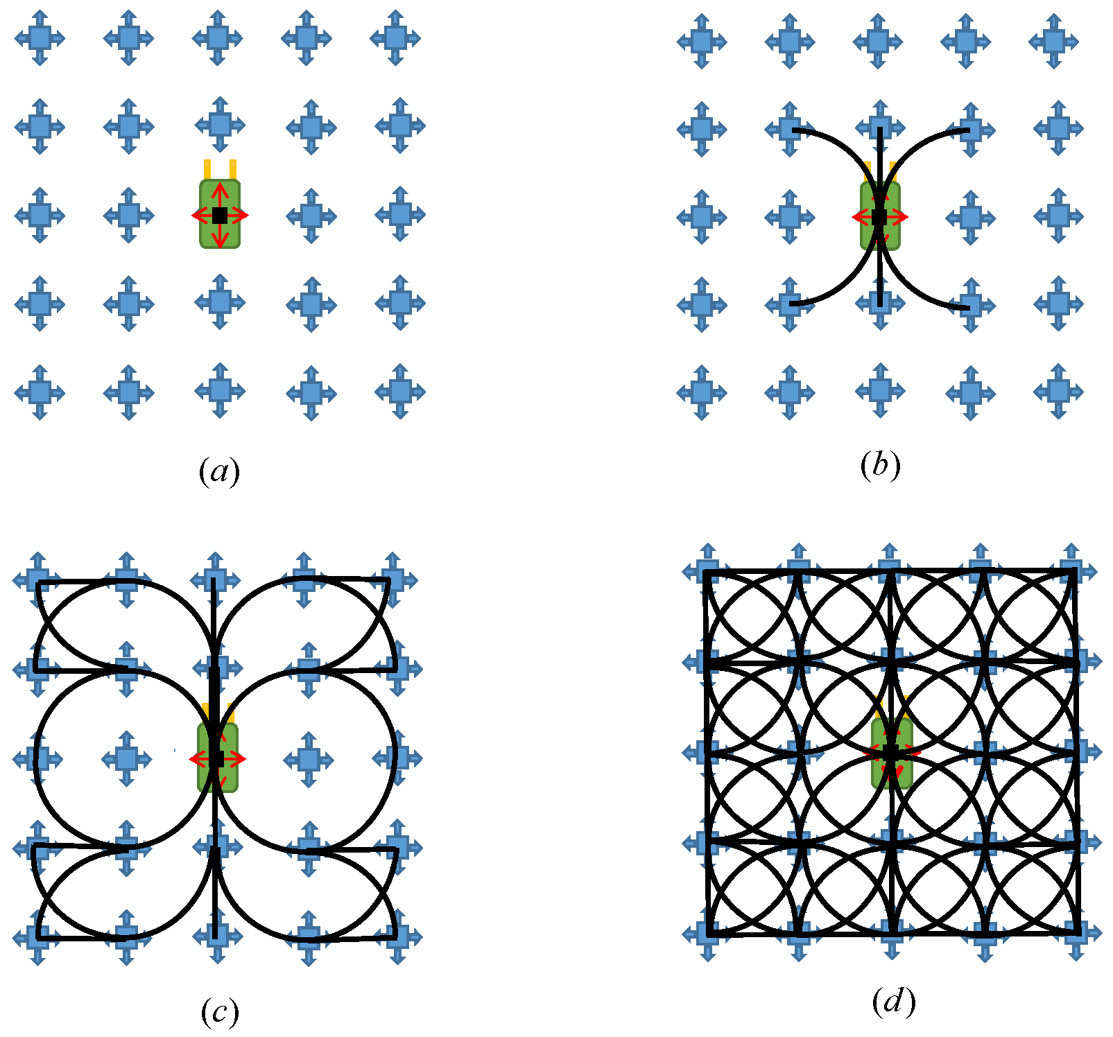
In our thesis, we construct a 4D state lattice based on the position (x, y), heading (
), curvature (k) for the kinematics model of the forklift. In order to simplify the construction process, we use a special discretization of state and control space [
28]. The orientation of the forklift is assumed to be uniformly distributed in space [0, 2
], and the discrete curvature K is also uniformly distributed between [
,
], where
.
Figure 4 shows the accessible graph for the forklifts with three actions. Due to the random position of the forklifts in autonomous navigation space, the state lattice is required to have spatial repeatability, motion primitives generated at a certain node can be applied to other nodes too. The motion primitives in
Figure 4 are generated by copying motion primitives from the starting point to other nodes, so the global paths generated by the control system are also feasible for the forklift. Through the generation of motion primitives in the state lattice, the global path planning problem is transformed into the path search and decision problem in different motion primitives, and then generate the feasible trajectory. Combined with the commonly used ARA* search algorithm, we can then obtain a path from the start point to the target that satisfies the kinematic constraints for the forklifts.
3.3. ARA* Path Search
Among the traditional path search algorithms, the A* algorithm is widely used in industrial fields because it can effectively solve the shortest path within a short time period. However, the heuristic functional construction of the A* algorithm was relatively simple, and there were more redundant nodes in the execution process of the algorithm, which were time-intensive and, thus, expensive to resolve. In order to achieve a rapid online solution, we employed the ARA* algorithm to search the path on an expanded raster map. The algorithm first found an optimal non-global feasible path under a given relaxation condition and then gradually strengthened the constraints in the remaining time, continuously improving the sub-optimal solution by using the searched node information. If it had sufficient time, the algorithm would find an optimal global feasible path. The algorithm reused the previous search results in the process of path optimization. The cost estimation function of the ARA* algorithm was improved, as compared to the A* algorithm. The cost estimation function was expressed as follows:
where
is the expansion factor, s represents the current node, f(s) is the cost from the starting point to the end point, g(s) is the actual cost from the starting point of the path to the current node, h(s) is the cost from the current node to the end point cost estimate. During the execution of the algorithm, the expansion factor
gradually decreases from the set initial value. If the algorithm can run for enough time, then finally
. If the runnable time is insufficient, then
will be as close to 1 as possible, and subsequently the obtained path is a suboptimal solution.
In this paper, the ARA* algorithm was used to search for a collision-free path in the state grid that satisfied the kinematics and time constraints for forklift travel, and the algorithm obtained the optimal solution within the time constraints.
3.4. Offline Pre-Computed Security Envelope Set
The safety envelope was an artificially determined convex polyhedron area that wrapped around the initial path, and the various poses of the robot in this area had to satisfy the kinematic model of the vehicle. During the path optimization step, the safety envelope was used for collision-avoidance constraints, so that the points on the path could be adjusted within the safety envelope. While calculating the optimal solution for local path optimization, this ensured that the optimized path avoided collisions. The correct setting of the safety envelope eliminated the safety hazards caused by the robots colliding at a smooth point due to trajectory optimization. However, safety envelope extraction has typically been a difficult and time-consuming process and has not been able to fulfill the needs of online trajectory generation for forklifts. In this study, a new algorithm for the rapid computation of path-space security envelopes was proposed. The algorithm divided the extraction of safety envelope constraints into two steps: an offline pre-computed safety envelope set and an online path-envelope extraction, both of which greatly improved the efficiency of safety envelope extraction.
The process of the entire security envelope extraction algorithm is shown in
Figure 5. After the path-planning module searched for an initial collision-free path, the pre-computed envelope set was used to extract constraints for each path point in collision-free path. Next, the safety envelopes of each position point in the path were superimposed to obtain the overall safety envelope [
29] of the path, which was then used as the optimization safety obstacle avoidance constraint for the next path. This section introduces the offline security envelope set calculation. The extraction process of the online path security envelope is detailed in the following subsections.
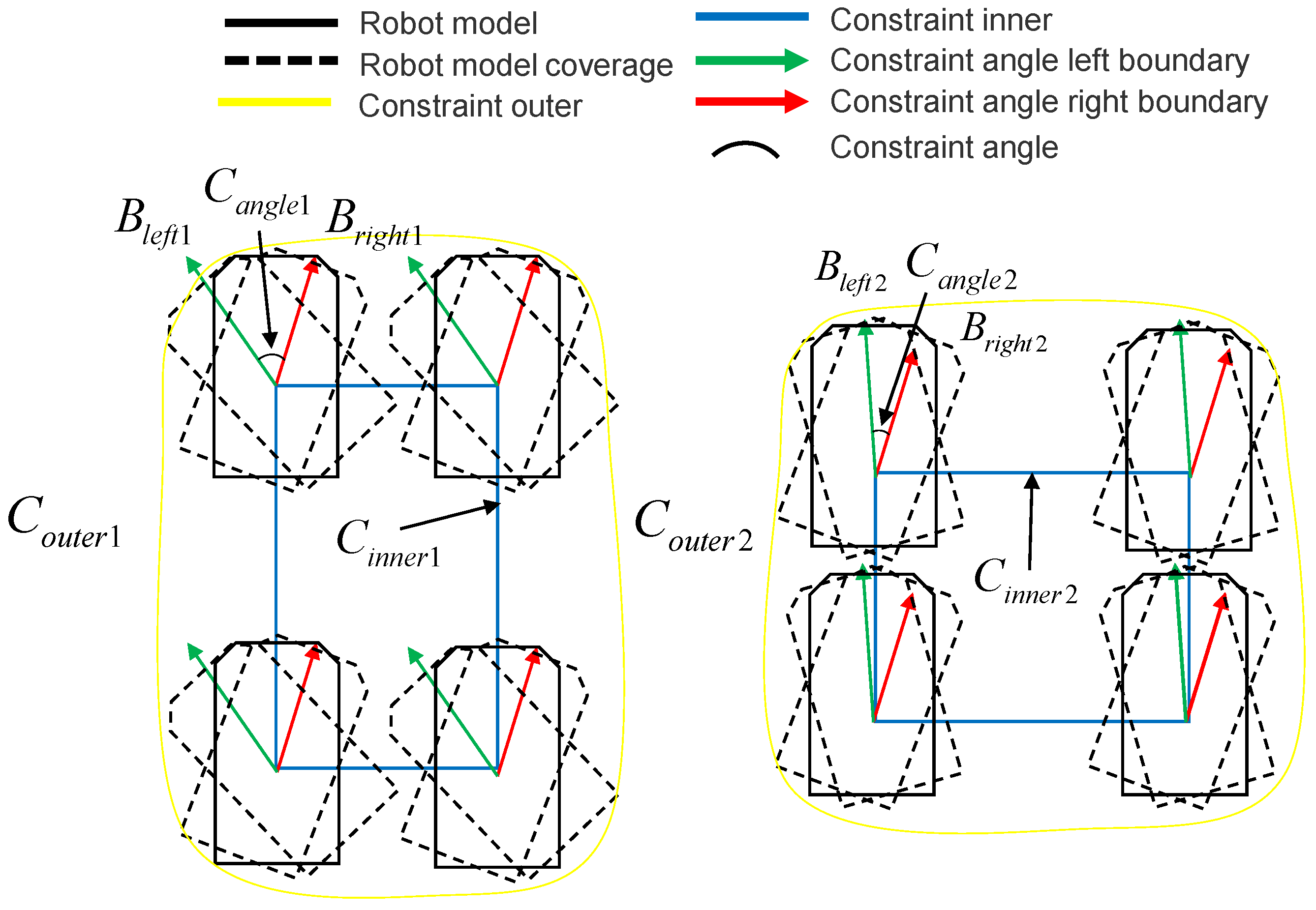
The pre-calculation module employed in this paper generated different robot envelopes according to different forklift models and corresponding load models, and also calculated a pre-set internal position constraint
and angle constraint
that were stored in the table. The size of the inner constraint
in the safety envelope constraint set
was the rectangle formed by the linear combination of the displacement of the forklift reference point in four directions; forward, backward, left, right, in addition to angle. The angle constraint
was the linear combination of the left and right offsets based on the direction of the forklift reference point. We arranged and combined the internal constraints
and the angle constraints
freely and, then, calculated the area and angle constraints
of each set of internal constraints
. We used their product as the weight
w of each constraint set and stored them in the security envelope constraint set
, in order of weight. Finally, according to the differences of the forklift envelopes, the outer constraints
generated by each pair of constraints were calculated. As shown in
Figure 6, the two graphs display the combination of the two kinds of internal constraints
(blue rectangle) and angle constraints
(red arrow and green arrow) in the lookup table, which generated a schematic diagram of the outer constraint
(yellow polygon). The algorithm flow is shown in Algorithm 1.
| Algorithm 1 Lookup table calculation |
- Input:
Lookup table: x Distance deviation: n1,n2,n3,n4,n5,n6,n7 y Distance deviation: m1,m2,m3,m4,m5,m6,m7 Angle deviation: Item: - 1:
Set constraint center - 2:
while do - 3:
for do - 4:
Set rectangle angle deviation is - 5:
Generate of element in - 6:
for do - 7:
Set rectangle length is - 8:
for do - 9:
Set rectangle width is - 10:
Generate of element in - 11:
Generate according to and - 12:
Calculate w of - 13:
- 14:
end for - 15:
- 16:
end for - 17:
- 18:
end for - 19:
Sort the elements in according to w - 20:
Output - 21:
endwhile - 22:
end while
|
3.5. Online Computed Path Security Envelope
Based on the pre-computed safety envelope constraint set obtained in the previous section, when the starting and ending points of the forklift navigation were provided, the motion planner searched for a kinematically feasible collision-free path. The path-envelope-generation module generated the safety envelope of the path according to the grid-map information, the original path, and the safety envelope constraint set PC. The safety envelope of a path was the collision-free free space region around the path, expressed in the form of a convex polyhedron constraint for the vehicle state, divided into an inner constraint and an angle constraint . Among them, the left boundary and the right boundary of the angle constraint limited the directions that the forklift, and the internal constraint defined the safe movement range of the forklift reference point during optimization. The constraint generation algorithm proposed in this paper defined a constraint combination formed by a space constrained by different positions and directions at each waypoint and then superimposed angles on the four vertices of the inner constraint . Through the forklift model constraint, the area covered by in all directions obtained the outer constraint of this point.
The definition of the internal constraint
is shown in the Equation (
6).
represents the vector between two points, where
,
n is the total number of path points.
P is the coordinates of the
i-th path point,
are the four vertices of the
rectangle.
The definition of the angle constraint
is shown in Equation (
7), and
is the angle of the path point.
The definition of the external constraint
is as follows (
8):
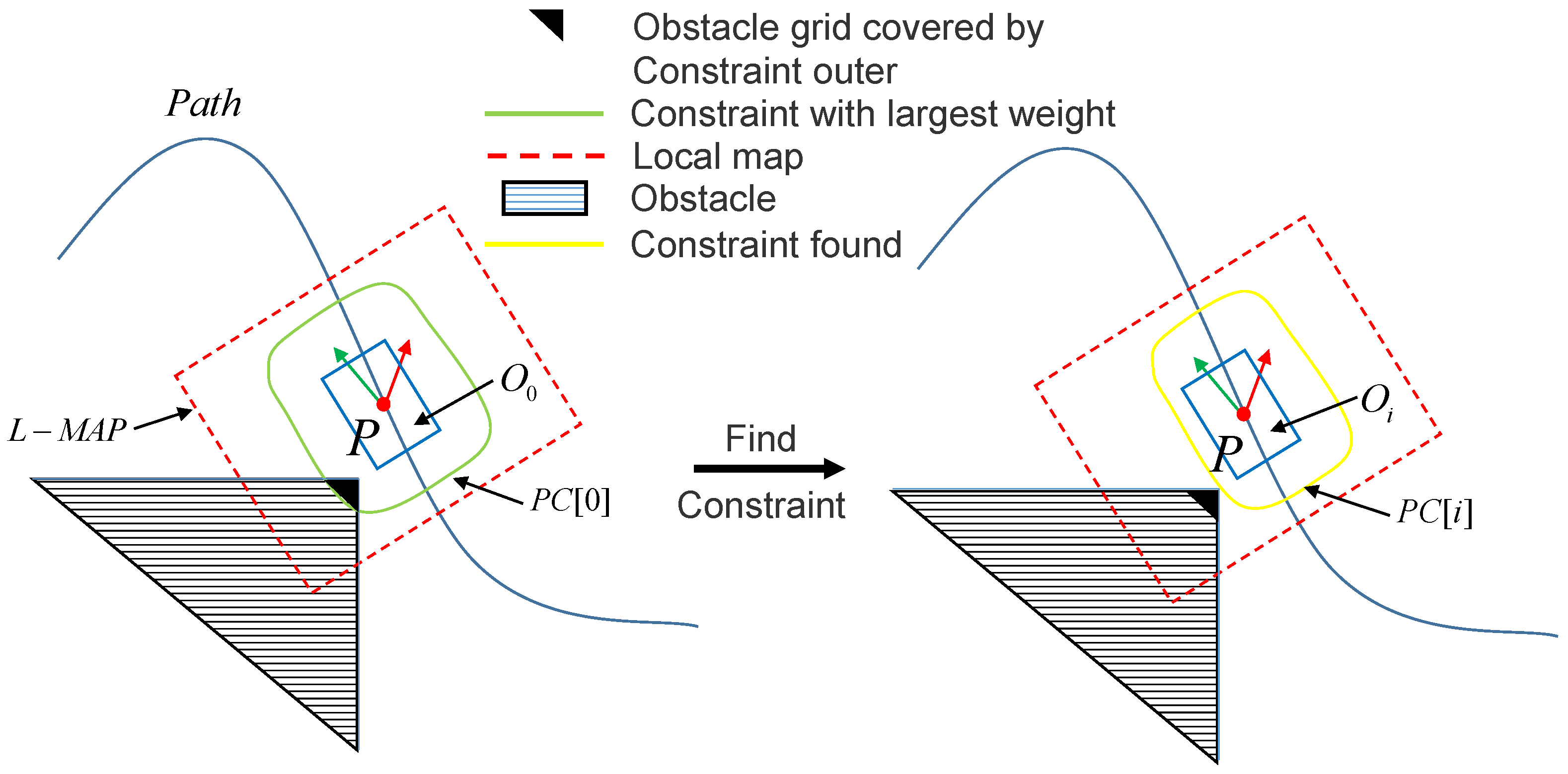
The above constraints defined all possible sets of safety envelopes for each waypoint in the original path of the vehicle, without considering obstacles. Next, we introduced the solution of the maximum safe envelope for each waypoint, considering obstacles. For each waypoint, our constraint generation algorithm generated a local map
at the point, which saved the largest external constraint
and set the grid
covered by the local map
in
to
and saved these
in array
. If we relocated the local map
to each waypoint
P and if
covered the obstacle grid on the world map, it would continue to traverse the next element in the security envelope constraint set
according to the weight
w. We followed this method until the
of the first uncovered obstacle corresponding to
in the safety envelope constraint set
was found, that is, the outer constraint
of this waypoint, which is shown in the following figure. Conversely, the maximum external constraint
was the constraint of the path point
P. The algorithm block diagram of the waypoint-finding constraints is shown in
Figure 7. The triangle area is the obstacle, the black area is the part covered by the external constraints of the robot, the red dotted line is the local map, the green line represents the largest external constraints in the PC, and the yellow line is the found external constraints. The safety envelope of the entire feasible path was obtained by superimposing the external constraints
of all path points. The secure envelope of the path is shown in
Figure 8. The algorithm flow is shown in Algorithm 2.
| Algorithm 2 Find constraint in path point P. |
- Input:
Lookup table: Item: - 1:
Generate local grid map with - 2:
Set in - 3:
Transfer in local map to P - 4:
Get obstacle grid array covered by - 5:
while do - 6:
for o in do do - 7:
if then - 8:
break - 9:
end if - 10:
if then - 11:
Output - 12:
end if - 13:
else - 14:
Continue - 15:
end else - 16:
if then - 17:
break - 18:
end if - 19:
if then - 20:
Error reporting - 21:
break - 22:
end if - 23:
- 24:
end while - 25:
end for - 26:
end while
|
3.6. Path Smoothing
This section introduces the implementation steps of the path-smoothing method based on optimization, which used the original path searched and considered constraints such as the starting point, target point, kinematics, dynamics, turning limit at the end of the path, and the path safety envelope of the robot, to generate a high-precision smooth path. The detailed process of imposing constraints was as follows. Given the starting point and target point , respectively, of the forklift by the task-scheduling system, the motion planner generated a collision-free kinematic path, and the path consisted of a series of state points. However, sampling-based non-holonomic motion-planning methods have generated paths that resulted in discretization errors and discontinuities within the paths themselves or between the stopping point and the goal state. This did not fulfill the requirements of end-pose accuracy required for industrial applications. Because the original path of the ARA* search was from a discretized starting state to a discretized target state , and represented the state points closest to and in the state grid map, respectively.
To solve this problem, we modified the starting and target states of the forklift to precisely correspond to the current vehicle state
and the actual target state
. Additional constraints were imposed during the path optimization function, as shown in Equation (
9). Equation (
9) effectively addressed the inaccuracy of the initial and final states caused by the discretization in state-grid-based motion planners.
In order to ensure that the planned path satisfied the kinematic and dynamic constraints of the forklift, additional constraints were imposed, as shown in Equation (
10):
In an industrial forklift with an under-actuated kinematic structure, it is relatively difficult to adjust the lateral deviation while driving. In order to improve parking accuracy, a docking point with a constant attitude is typically added before the parking point to ensure that the vehicle continues in a straight line at the end of the path. The method of adding docking points at the end of the path improved the parking accuracy; however, it also increased the difficulty of operation and reduced efficiency. In order to solve the problems of planning efficiency and parking accuracy at the same time, we imposed steering-angle constraints on the state points at the end of the trajectory, as shown in Equation (
11):
It was assumed that the distances between the state points of the path were approximately equal, and the time
between the consecutive state points was set to any fixed positive value. Therefore, the time
T through the entire path was set to a constant value
.The optimal control function of the forklift is shown in Equation (
12), and the constraint term of the optimization function is shown in Equation (
13), where
is a weighting factor of adjusting the minimum travel distance and minimum rotation of the forklift;
is the left boundary of the angle constraint of the
i path point;
is the right boundary of the angle constraint of the
i path point;
b,
,
are intermediate variables, such as in Equation (
6),
is the inner constraint of the
i path point,
P is the coordinates of the waypoint,
are the vertices of the rectangle:
Our optimization variables were the forklift’s front wheel’s travel speed
v and angular velocity
w, and the goal was to minimize the total travel distance and the amount of rotation imposed on the front wheel angle of the forklift. The objective function in Equation (
12) minimized the combination of the total distance traveled by the forklift and the total steering wheel rotation.
The optimal control Equation (
12) and the constraint item (
13) were optimized and calculated as the optimal path-state point
. The optimized state point
was the obtained smooth path point.
After feeding
into a trajectory generator, we used the trajectory generator from
Section 3.7 to generate a set of values for each state in the path, given the constraints of the initial and final velocities, steering velocity, steering acceleration, velocity, and acceleration, to allocate the maximum speed.
3.7. Trajectory Generation and Track
After the planner generates a series of discrete state points at fixed intervals, the trajectory generator output a trajectory with a fixed
of 50 ms as the input to the controller [
30,
31]. As previously mentioned, there are two types of trajectory generation methods typically used in the literature: trajectory generation based on a polynomial function and trajectory generation based on a B-spline curve.
The trajectory generation based on a polynomial function generated the operating trajectory of the forklift by calculating the polynomial coefficients that satisfied the constraints and drew on the polynomial function. However, in order to ensure the safety of the forklift, this method required multiple iterations, which was considerably time-consuming.
The curvature of the B-spline curve was continuous at the nodes of adjacent curve segments, and if the local constraints of the trajectory were not satisfied, the trajectory could be corrected by adjusting the corresponding control points without affecting other trajectory segments [
32]. Among them, the cubic B-spline curve exhibits the characteristics of second-order continuity at the nodes, which could optimize the curve and meet the requirements of the acceleration and speed continuity of a moving unmanned forklift. Therefore, the trajectory generator employed in this paper was the cubic B-spline curve.
In this paper, the model predictive control (MPC) method was used to realize trajectory tracking [
33,
34,
35,
36]. Given a set of state inputs, the controller then used an objective function based on the tracked trajectory to optimize the control output. Since the controller is not the focus of this article, we have not provided the relevant theoretical exposition.
4. Experimental Evaluation
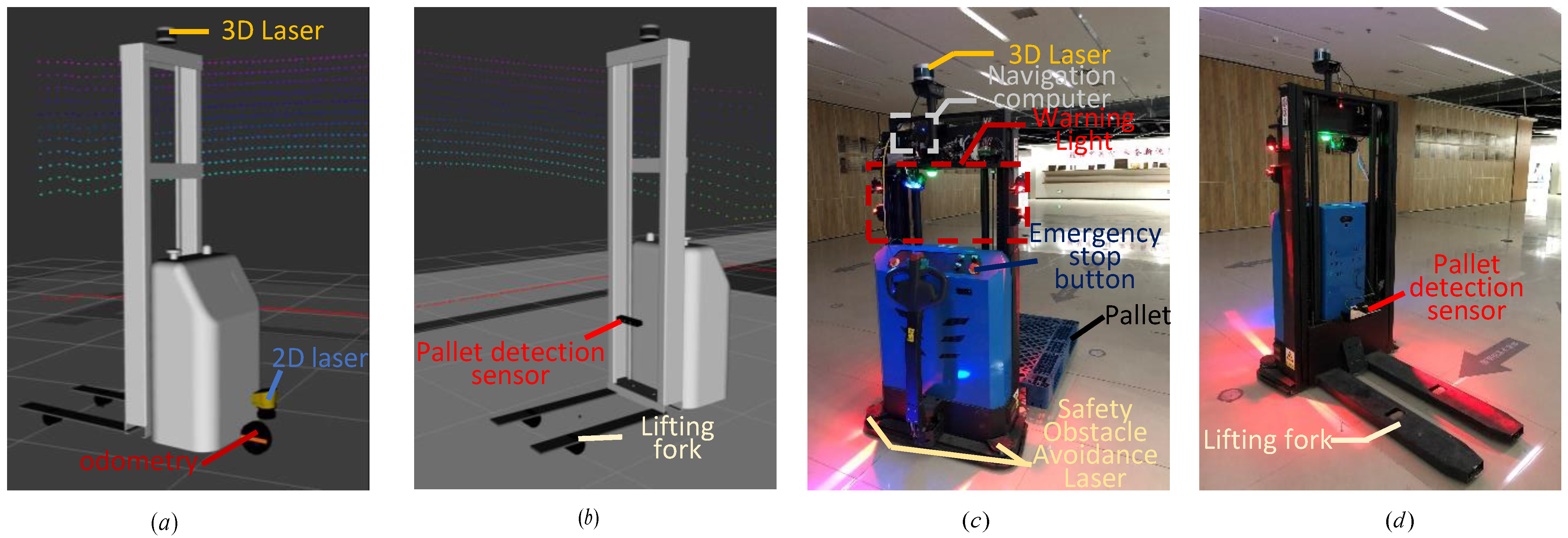
In order to fully evaluate the comprehensive performance of the algorithm proposed in this study, an experimental verification of the algorithm was carried out in simulated and real environments. The navigation algorithm was operated on a personal computer with an Ubuntu 16.04 operating system, an i5-6200u CPU, 8 GB of RAM, and 512 GB storage space. The entire navigation system was implemented within the Robot Operating System (ROS). In the simulation experiment, a forklift model that satisfied the car-like kinematics was created, and a gazebo simulation environment was built. The experiment was equipped with a high-precision locator, the translational positioning accuracy was within 1cm, the rotation angle positioning accuracy was 0.001 radians, and the on-board navigation control system could access the encoder and positioning data. In the real-world environment, the modified industrial unmanned forklift was equipped with three on-board lasers, two of which were safety lasers located on the ground for safe parking in emergency situations. The second navigation laser was an RS-LIDAR-16, a 3D laser rangefinder with a viewing angle of 360 degrees and 16 lines. The communication between the navigation computer and the motor driver through CAN bus was used to collect odometer data and control vehicle motion, and an Ethernet interface was used to transmit LiDAR distance data. Therefore, the navigation computer received encoder and positioning data and sent steering and driving commands, as shown in
Figure 9.
The overall goal of our experimental evaluation was to demonstrate the real-time performance, reliability, and accuracy of online-generated trajectories. We divided the experimental evaluation into four parts. (1) Path-smoothing evaluation, which considered the importance and realization of path smoothing; (2) random-target experimental evaluation to further test the robustness of our system on arbitrary target poses and longer distances; (3) obstacle extension evaluation to analyze the operation of the system in more challenging scenarios; and (4) the evaluation of real pallet fork-and-pick tasks.
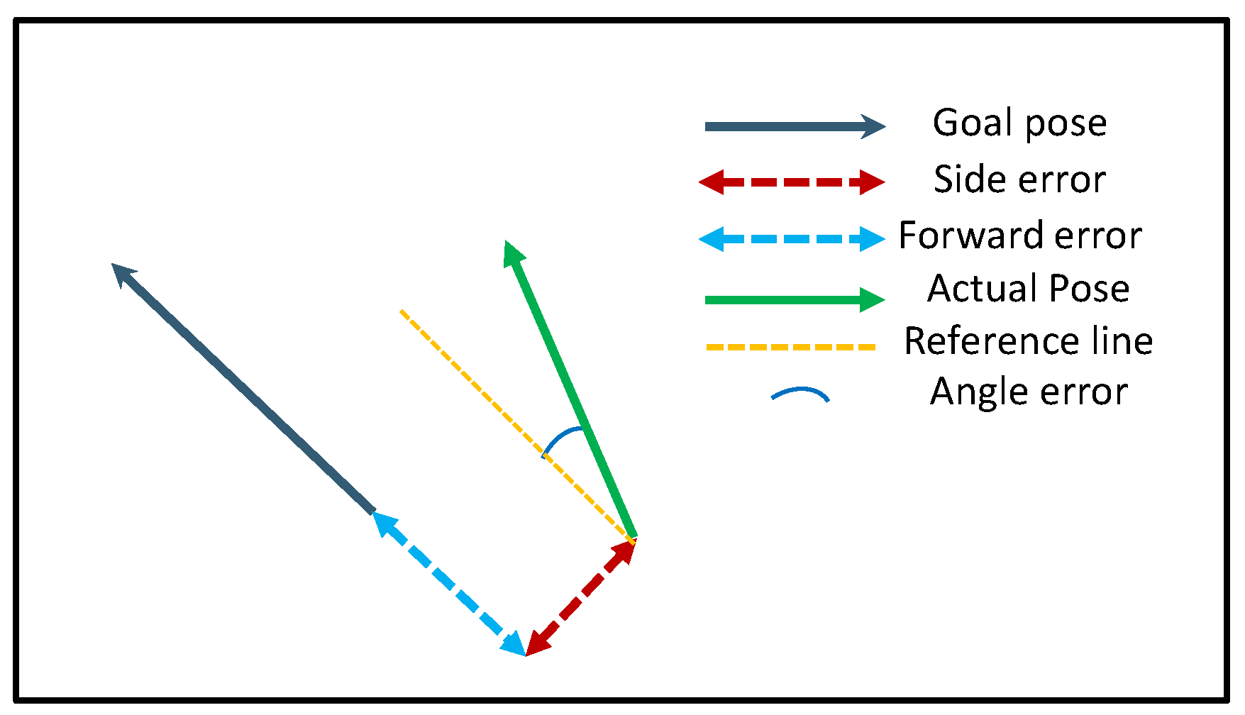
For a non-holonomic vehicle, it was difficult to control the direction and the position perpendicular to the motion direction, which was convenient for analyzing the data. We decomposed the errors into forward errors, lateral errors, and heading errors, as shown in
Figure 10. For each type of error, we showed the results in terms of mean, standard deviation, and maximum value obtained during the test operation.
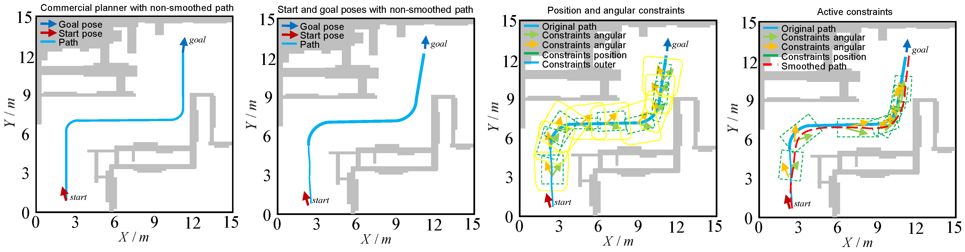
4.1. Path-Smoothness Evaluation
In this experiment, the importance and implementation of path smoothing were evaluated. Our focus centered around the accuracy of the online trajectory planning and tracking reaching the accuracy of offline trajectory planning and tracking while fulfilling the requirements of industrial applications. We extracted 10 sets of target poses from hand-defined paths (shown on the left of
Figure 8) and used them as targets for a lattice-based motion planner. The output of the motion planner was passed to a path smoother, which was then tracked by the MPC controller. Note that when the path was not processed by the smoother, in order to ensure the parking accuracy, the target state was set as the last point of the trajectory, thus allowing the MPC controller to correct the motion direction caused by the rough path.
The experimental results are shown in
Table 1 as a comparison of the results obtained by the motion planner, with and without path smoothing. The error description is shown in
Figure 10, which depicts the forward, lateral, and heading errors between the target position and the final parking point. These results confirmed that our system could produce smooth trajectories with excellent end-pose accuracy, with improvements in forward, side, and orientation errors, as compared to no smoothing. Our method could completely replace navigation systems that generate paths manually, without loss of accuracy. (In typical factory settings, the positional accuracy required by the forklift to pick up the pallet was 0.03 m, and the direction accuracy was 0.017 rad [
37]). The experimental results further showed that it was necessary to use path smoothing in order to obtain high accuracy of the final parking attitude.
4.2. Randomized Target Experimental Evaluation
To further test the robustness of our system for arbitrary target poses and longer distances, we used two test scenes, as shown in
Figure 11, each with two blocks marked by dashed lines area. A total of 20 target groups were randomly generated between two areas. The vehicle was tested in two scenarios, from one area to another, reciprocating between multiple poses, and a total of 40 paths were tested.
The experimental results obtained are given as follows. The forward, lateral, and heading errors are shown in
Table 2 while the motion-planning time, path-constraint-extraction time, and path-optimization time are shown in
Table 3.
Table 2 compares the improvement ratio of various indicators before and after path smoothing, with the average improvement value being 92.42%.
Figure 12 is a visual description of
Table 3. The experimental results indicated that the proposed path-smoothing method had high robustness and great improvements in parking errors, even when the maximum position accuracy error was less than 3 cm. In addition, the total time demand of path planning was shortened, which fulfilled the real-time and precision requirements of online path generation for forklifts.
4.3. Barrier Extension Assessment
In order to test the operation of our method in more challenging scenarios, we conducted experimental evaluations in narrower and longer scenarios with additional obstacles, as shown in
Figure 13. In the figure, the shaded part is the additional obstacle, as expected, due to the more complex space of these two test scenes; the deviation of the smoothed path from the original path is smaller, and the number of space constraints is higher. The experimental results showed that the planning method proposed in this paper was also effective in more challenging scenarios.
4.4. Real Pallet Fork Experiment
In order to verify the reliability and robustness of our proposed algorithm for performing real tasks, we carried out a flexible fork-and-pick experiment on a pallet in a 600-square-meter experimental test site. The selected tray specifications were as follows: grid plastic tray, 1.2 m long, 1.2 m wide, and 0.155 m high. We used a high-precision pallet recognition-and-positioning system: The recognition frequency was 1 HZ, the recognition position accuracy was 0.008 m, and the attitude accuracy was ±1.5 degrees.
The starting point Ps was defined in the experimental site, the photographing point Pa was fixed, the real pallet position point Pr was recognized, and the fork adjustment point Pd was automatically generated, as shown in
Figure 14. In each fork-and-pick experiment, the pallet placement position was set within a certain position and attitude deviation relative to the photo point (position deviation ≤ 0.2 m, attitude deviation ≤ 0.5 rad), and the forklift navigated from any position Ps on the site to the photo point Pa. Actions, such as image captures, the flexible adjustment of poses, and the tray insertion, were completed successively. After 10 random pallet fork experiments, including the empty space near the pallet placement position (as shown in
Figure 15) and the more difficult challenge of a tray placed near the wall (as shown in
Figure 16), the task success rate was 100%.
5. Conclusions and Future Works
Current forklift trajectory planning systems that use offline generation have been unable to provide flexible, smooth route planning. We therefore proposed and designed a new flexible online trajectory planner for industrial forklifts in this study. There are two main advantages offered by our proposed method:
(1) It operates online. From the front-end original path search to the back-end path optimization, time constraints were considered. The online search employed the ARA* method to ensure search-time constraints. The time-consuming space safety envelope was divided into two steps involving the offline calculation of the envelope set and the online generation of the path safety envelope. The safety envelope constraint with position and attitude angles was directly added to the back-end path optimization, which effectively eliminated the second verification step of trajectory after the path had been smoothed. Additional curvature constraints were incorporated into the path optimization process, thus no secondary curvature evaluations were required on the final path. These steps ensured the overall time efficiency of the online trajectory generation.
(2) It demonstrates high precision. The trajectory planner designed in this paper was conducted online, which improved the accuracy, smoothness, and security of planning. The front-end path search used a sampled-state lattice-based path-search method. The original path search satisfied the kinematic constraints of the vehicle; however, problems such as discretization errors and curvature discontinuities occurred on the path itself or between the parking point and the target state. This did not fulfill the end-pose accuracy requirements for industrial applications. The back-end optimization method smoothed the path. The state constraints of the starting and the target points were added to the path optimization, which ensure the pose accuracy of the optimized path at the starting and the target points. Before the fork point, by imposing corner constraints to ensure smoothness of the end path, the parking attitude accuracy of the target point was effectively improved. These steps ensured high precision of the trajectory generated by the navigation system.
In our future research, we plan to improve the execution of the navigation task as well as reduce execution time. At present, the pursuit of refined controls in digital factories for the transportation of goods is directly connected with production and assembly. In order to improve overall production and handling efficiency, the factory’s task scheduling system not only sends handling instructions to the forklift, but also issues the time required to complete the navigation task. Therefore, the execution of navigation tasks with time constraints is critical to achieving improved production efficiency, assembly, and transportation in future intelligent factories.


